A PHM System Approach: Application to a Simplified Aircraft Bleed System

O

pen

A

rchive

T

OULOUSE

A

rchive

O

uverte (

OATAO

)

OATAO is an open access repository that collects the work of Toulouse researchers and

makes it freely available over the web where possible.

This is an author-deposited version published in :

http://oatao.univ-toulouse.fr/

Eprints ID : 15670

To link to this article :

http://ieeexplore.ieee.org/Xplore/home.jsp

To cite this version : Maitre, Josselin and Sen Gupta, Jayant and

Medjaher, Kamal and Zerhouni, Noureddine A PHM System

Approach: Application to a Simplified Aircraft Bleed System. (2016)

In: 2016 IEEE Aerospace Conference, 5 March 2016 - 12 March

2016 (Big Sky, United States).

Any correspondence concerning this service should be sent to the repository

administrator:

staff-oatao@listes-diff.inp-toulouse.fr

A PHM System Approach:

Application to a Simplified Aircraft Bleed System

Josselin Maitre ENSMM 26 rue de l’Epitaphe 25000 Besançon, France josselin.maitre@gmail.com

Jayant Sen Gupta Airbus Group Campus Engineering

18 rue Marius Terce 31300 Toulouse, France jayant.sengupta@airbus.com

Kamal Medjaher, Noureddine Zerhouni FEMTO-ST Institute

UMR CNRS 6174 – UBFC / UFC / ENSMM / UTBM 24, Rue Alain Savary

25000 Besançon, France {kamal.medjaher, zerhouni}@ens2m.fr

Abstract— Regarding Prognostics and Health Management (PHM), the stakes lie in system-level prognostics or even the prognostics of systems of systems, as decisions are usually made at system or platform level. In this paper, a method, which takes into account both the system redundancy and the adaptation of operational modes in degraded functioning, is proposed and formalized. This method makes the system-level prognostics more relevant. The main feature of the method is to re-compute the components Remaining Useful Life (𝑹𝑹𝑹) using the degradation rate associated to the future operating mode(s) due to system reconfiguration. This results in an improvement of both the System 𝑹𝑹𝑹 (𝑺𝑹𝑹𝑹) and the components 𝑹𝑹𝑹. The proposed method is applied on a simplified aircraft bleed valve system to illustrate its effectiveness. This method is primarily destined to aeronautic systems, which are usually resilient. It has not been tested whether or not it could be useful in other fields.

T

C

I

... 1

C

F

... 1

P

A

... 3

C

S

... 5

C

... 7

R

... 8

B

... 9

I

Aircraft Operability is a critical aspect for airlines, especially nowadays as the traffic is getting more and more congested on airports and the time windows allowed for taking-off are tighter. In this scope, aircraft manufacturers tend to improve aircraft operational reliability by implementing more predictive maintenance on their aircraft, through services for instance, in order to reduce unscheduled maintenance. Instead of replacing a device at a planned date (scheduled maintenance) or when it is faulty (corrective maintenance), predictive maintenance consists in monitoring the health rate of each individual component (or system) and predict its future states by taking into account future missions in order to replace it just before a failure occurs. This is the main purpose of Prognostics and Health Management (PHM) [1 – 4].

In this scope, one needs to estimate and predict the health state of an aircraft system component by component. The

Remaining Useful Life (𝑅𝑅𝑅) is one of the classical prognostics output that can be computed for a component [5 – 9]. In order to assess the impact on operability, the component fault is not the correct indicator. Indeed, the operability is only impacted by the loss of an important function, thus the Remaining Useful Life at system level (𝑆𝑅𝑅𝑅) is a more relevant indicator. Nevertheless, even though it would be the right level to deal with, computing the 𝑆𝑅𝑅𝑅 is still a challenge.

Several factors explain this difficulty. First, assessing the prognostics of all critical components in a system is not always trivial. Second, components interact in the system and modeling these interactions can become a very complex task. Finally, systems have different operating modes that are not always easy to take into account. For instance, aeronautical systems are resilient to component faults thanks to material redundancy. By duplicating the components performing a task, several faults of the same type of component are necessary to cause a system failure. But material redundancy is costly in terms of weight as it requires doubling or tripling the number of components. Another way is to adapt the operating mode to the number of remaining items, soliciting more and more the components as there are fewer items to perform the task. Therefore, simply computing the 𝑆𝑅𝑅𝑅 as the minimum value of the system components 𝑅𝑅𝑅 is not accurate. Likewise, computing the minimum value of components 𝑅𝑅𝑅 in a degrading system is not a trivial task. This is because the system reconfigures in degraded modes to maintain its function, thus changing some components operating mode and therefore changing their degradation rates and 𝑅𝑅𝑅. In other words, the 𝑅𝑅𝑅 of a component in a system depends on the future states of the system.

We will first explain the context of this paper, then develop the proposed method for system-level PHM, and finally illustrate with an application to a case study.

C

F

Definitions

Several specific terms will be used in the following development, they will be defined here.

A health indicator 𝐹_𝑖 is a relation between several physical parameters,𝛼₁, … , 𝛼_𝑚 that represent the degradation of a component. It is defined with an associated threshold 𝑇_𝑖, above which the related component is considered faulty. The health state ℎ_𝑖 of a component 𝐶_𝑖 is the value of its health indicator at a defined point in time:

𝒉𝒊(𝒕) = 𝑭𝒊�𝜶𝟏, (𝒕) … , 𝜶𝒎(𝒕)� (1)

and its state 𝑧_𝑖 is either functioning: 𝑯𝒊< 𝑻𝒊⇒ 𝒛𝒊= 𝟏 (2)

or faulty:

𝑯𝒊> 𝑻𝒊⇒ 𝒛𝒊= 𝟎 (3)

A system of 𝑛 components has 𝑞 = 2𝑛 states 𝑍₁, … , 𝑍_𝑞 where each system state:

𝒁𝒋= �

𝒛𝟏

⋮ 𝒛𝒏

� 𝝐 {𝟎, 𝟏}𝒏 ₍₄₎

is a vector containing the 𝑛 components states. The space: 𝓩 = � 𝒁𝟏, … , 𝒁𝒒� (5)

can be divided into two sub-spaces 𝑍_{𝑓𝑓𝑓𝑓𝑓𝑓} and 𝑍_{𝑓𝑓𝑛𝑓} corresponding respectively to the states leading to a system failure and the states in which the system functions.

The evolution of the health state ℎ_𝚤̇ corresponds to a certain degradation rate. An associated degradation function 𝑑_𝑖 represents its evolution in time so that:

𝒉𝒊̇ = 𝒅𝒊(𝒑𝒑𝒑𝒑𝒎𝒑𝒕𝒑𝒑𝒑) (6)

and allows computing the health state at a certain future time ℎ_𝑖�𝑡_{𝑓𝑓𝑓𝑓𝑓𝑓}�. In practice, under the hypothesis that the operating condition stay the same in the future, ℎ_𝑖�𝑡_{𝑓𝑓𝑓𝑓𝑓𝑓}� can be computed using a history of health states and interpolating it to obtain a trend for future times, for example by linear regression.

The health state evolution depends a priori on the health state of every component of the system, so that:

𝒉𝒊̇ = 𝒅𝒊(𝒉𝟏, … , 𝒉𝒊, … , 𝒉𝒏). (7)

Reminder on Component-Level 𝑅𝑅𝑅 Computing

The starting point of a system-level 𝑅𝑅𝑅 computing is the component-level 𝑅𝑅𝑅 computing. To compute it, in practice, the health state history of a component 𝐶 is interpolated and the resulting function is used to determine when the health indicator will reach the threshold. The time elapsed until then defines the 𝑅𝑅𝑅.

In the literature, only few methods are proposed to compute a system-level prognostic [10 – 14].

Methods to Compute System-Level 𝑅𝑅𝑅

In this part, we will review the methods already existing and usually used to compute a 𝑆𝑅𝑅𝑅.

In most existing methods, a recurrent simplifying hypothesis consists in considering that the components degradations are independent from one another. This amounts to considering that, for a component 𝐶_𝑖, the health indicator evolution 𝑑_𝑖 only depends on the corresponding ℎ_𝑖, that is to say:

𝒉̇ = 𝒅𝒊 𝒊(𝒉𝟏, … , 𝒉𝒊, … , 𝒉𝒏) = 𝒅𝒊(𝒉𝒊). (8)

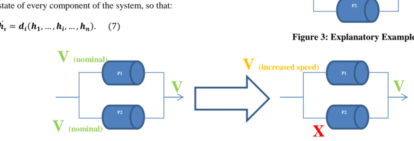
In order to explain them concretely, the methods will be accompanied by a system consisting in two pumps mounted in parallel, shown on Figure 3 below.

Figure 2: Component-Level 𝑹𝑹𝑹 Computing

P1

P2

Figure 3: Explanatory Example

P1 P2

V

V

V

X

V

V

ation

For safety and reliability reasons, most systems in aeronautics are either redundant (several components have the same function) or reconfigure in degraded states or both, which is usually the case. These systems are called resilient. In order to make this explanatory system more realistic, we will consider that it is resilient. Indeed, when a pump fails, the system will carry on functioning (redundancy), but the remaining pump will rotate with an increased speed to do so while meeting the required performance (reconfiguration). Therefore only a failure of both pumps will cause a system failure.

In Case of No Redundancy—A first method considers that:

𝓩𝒇𝒇𝒏𝒇= ��

𝟏 ⋮

𝟏��, (9)

meaning that the system is only considered functioning when every component functions.

In this method, a 𝑅𝑅𝑅 is computed for each component 𝐶1, … , 𝐶𝑛 as a list of component-level 𝑅𝑅𝑅 and the 𝑆𝑅𝑅𝑅 is

their minimum:

𝐶𝐶𝐶𝐶𝐶𝑛𝐶𝑛𝑡𝐶 = [𝐶1, … , 𝐶𝑛]

𝐹𝐶𝐹 𝑖 𝑖𝑛 𝐶𝐶𝐶𝐶𝐶𝑛𝐶𝑛𝑡𝐶: 𝐶𝐶𝐶𝐶𝐶𝑡𝐶 𝑅𝑅𝑅𝑖

𝑆𝑅𝑅𝑅 = 𝐶𝑖𝑛𝐶𝐶𝑚𝐶𝐶𝑛𝑓𝑛𝑓𝐶 (𝑅𝑅𝑅𝑖)

Applying this method to the explanatory system amounts to considering that:

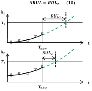
𝑺𝑹𝑹𝑹 = 𝑹𝑹𝑹𝟐. (10)

The fact that this system is redundant makes it irrelevant for this system. Indeed, 𝑆𝑅𝑅𝑅 is defined as the time remaining until the system fails which is not the case when a single pump fails according to the system definition.

The fact that most systems are redundant in aeronautics (which is our field of study) results in a strongly underestimated 𝑆𝑅𝑅𝑅, thus making this method irrelevant,

albeit conservative, as the 𝑅𝑅𝑅 computed with this method will always be smaller than 𝑆𝑅𝑅𝑅.

In Case of Redundancy—A second method takes into account the system redundancy, meaning that 𝑍_{𝑓𝑓𝑛𝑓} is not only equal to ��

1 ⋮

1�� as the redundancies allow the system to function even if some components are faulty.

This method uses the same algorithm as the first one and adds a test if the system state is included in 𝑍_{𝑓𝑓𝑓𝑓𝑓𝑓} in order to define 𝑆𝑅𝑅𝑅 as the time at which the system has a failure: 𝐶𝐶𝐶𝐶𝐶𝑛𝐶𝑛𝑡𝐶 = [𝐶1, … , 𝐶𝑛] 𝐹𝐶𝐹 𝑖 𝑖𝑛 𝐶𝐶𝐶𝐶𝐶𝑛𝐶𝑛𝑡𝐶: 𝐶𝐶𝐶𝐶𝐶𝑡𝐶 𝑅𝑅𝑅𝑖 𝑊ℎ𝑖𝑖𝐶 Z𝜖𝒵𝑓𝑓𝑛𝑓: 𝑖𝑓𝑚𝐶= 𝑎𝐹𝑎𝐶𝑖𝑛𝐶𝐶𝑚𝐶𝐶𝑛𝑓𝑛𝑓𝐶 (𝑅𝑅𝑅𝑖)) 𝑆𝑅𝑅𝑅𝑓𝑚𝐶= 𝑅𝑅𝑅𝑖𝑡𝑡𝑡 𝑅𝐶𝐶𝐶𝑅𝐶 𝐶_{𝑖𝑓𝑚𝐶} 𝑓𝐹𝐶𝐶 𝐶𝐶𝐶𝐶𝐶𝑛𝐶𝑛𝑡𝐶 𝑍�𝑖𝑓𝑚𝐶� = 0 𝑆𝑅𝑅𝑅 = 𝑆𝑅𝑅𝑅𝑓𝑚𝐶

According to the definition of the explanatory system: 𝓩𝐟𝐟𝐟𝐟𝐟𝐟= ��𝟎𝟎��. (11)

Therefore SRUL is the maximum of both pumps 𝑅𝑅𝑅: 𝑺𝑹𝑹𝑹 = 𝑹𝑹𝑹𝟏. (12)

This method improves the 𝑆𝑅𝑅𝑅 accuracy compared to the first one, since it takes into account the system redundancy. However, it does not take into account the possible reconfigurations. As an example, for the previous system, if the second pump increases its rotation speed when one fails, it might increase its degradation rate, and therefore the real 𝑅𝑅𝑅 of this component would be smaller than the computed 𝑅𝑅𝑅.

Therefore, this method might not be conservative due to the system reconfigurations, which makes it irrelevant as well.

P

A

Assumptions

The first assumption made in the method developed in this paper is that the operational conditions are the same between the different points at which the physical parameters are measured. That is to say, the degradation is not influenced by the aircraft operational conditions.

The second hypothesis is that 𝑍_{𝑓𝑓𝑛𝑓} is not only equal to ��1⋮

1��. This assumption allows taking into account the system redundancy, as explained earlier in the second method.

Finally, the third assumption is that, for a component 𝐶_𝑖, the health indicator evolution do not depend only on ℎ_𝑖, but also on components states 𝑧₁, … 𝑧_𝑖−1, 𝑧_𝑖+1, … , 𝑧_𝑛, that is to say:

𝒉𝒊̇ = 𝒅𝒊(𝒛𝟏, … 𝒛𝒊−𝟏, 𝒉𝒊, 𝒛𝒊+𝟏, … , 𝒛𝒏). (13)

This assumption is closer to reality compared to the second method and will allow adding relevancy to the computed SRUL. Under this assumption, a new notation can be used:

𝒅𝒊(𝒛𝟏, … 𝒛𝒊−𝟏, 𝒉𝒊, 𝒛𝒊+𝟏, … , 𝒛𝒏) = 𝒅𝒊𝒁(𝒉𝒊) (14)

where 𝑑_𝑖𝑍 represent the values taken by 𝑑_𝑖 when:

𝒁 = ⎝ ⎜ ⎜ ⎜ ⎛ 𝒛𝟏 ⋮ 𝒛𝒊−𝟏 𝟏 𝒛𝒊+𝟏 ⋮ 𝒛𝒏 ⎠ ⎟ ⎟ ⎟ ⎞ . (15)

The innovation of the method lies in this assumption, which means that the system reconfiguration is taken into account. It is interesting to note that this third assumption is an intermediate step between:

𝒉𝒊̇ = 𝒅𝒊(𝒉𝒊) (16)

And:

𝒉𝒊̇ = 𝒅𝒊(𝒉𝟏, … , 𝒉𝒊, … , 𝒉𝒏), (17)

As the components states are a discretization of the health indicators.

This intermediate assumption allows a simplification of application while not losing the relevancy of the result. Inputs of the proposed method

In order to use this method, a complete model of the system is not needed, neither is a precise knowledge of an indicator. These are some of the interests brought by this method. Some parameters are needed to initialize this method. First, one needs a history of the health state ℎ_𝑖 for each component, without needing to know how it was obtained but only to initialize the computing.

Then, one needs the degradation function 𝑑_𝑖 for each component 𝐶_𝑖, that is to say every of the degradation functions.

Finally, one needs to know the system states leading to a system failure: 𝑍_{𝑓𝑓𝑓𝑓𝑓𝑓}.

These parameters are enough to use the described method, note that no model of the system is needed. No deep knowledge of the system is needed; neither is knowledge of its architecture and functioning, as these data are completely transparent in the system.

Proposed Algorithm

The ground of this method and its innovation compared to previous methods is to take into account the system reconfiguration according to the system state. Therefore, under the third assumption presented in part 2, the components 𝑅𝑅𝑅 are re-computed with the updated degradation functions each time the system state changes. An important thing to point out is that every calculation is done at the same instant; the algorithm only simulates the future failures and system state changes.

The algorithm describing this method is the following:

𝑍 = �𝑧⋮1 𝑧𝑛 � = 𝑍𝑗 𝐶𝐶𝐶𝐶𝐶𝑛𝐶𝑛𝑡𝐶 = [𝐶1, … , 𝐶𝑛] 𝐹𝐶𝐹 𝑖 𝑖𝑛 𝐶𝐶𝐶𝐶𝐶𝑛𝐶𝑛𝑡𝐶: 𝐶𝐶𝐶𝐶𝐶𝑡𝐶 𝑅𝑅𝑅𝑖 𝑤𝑖𝑡ℎ 𝑐𝐶𝐹𝐹𝐶𝑛𝑡 𝑑𝐶𝑎𝐹𝑎𝑑𝑎𝑡𝑖𝐶𝑛 𝑓𝐶𝑛𝑐𝑡𝑖𝐶𝑛𝐶 𝑊ℎ𝑖𝑖𝐶 Z𝜖𝒵𝑓𝑓𝑛𝑓: 𝑖𝑓𝑚𝐶= 𝑎𝐹𝑎𝐶𝑖𝑛𝐶𝐶𝑚𝐶𝐶𝑛𝑓𝑛𝑓𝐶 (𝑅𝑅𝑅𝑖)) 𝑆𝑅𝑅𝑅𝑓𝑚𝐶= 𝑅𝑅𝑅𝑖𝑡𝑡𝑡 𝑅𝐶𝐶𝐶𝑅𝐶 𝑖𝑓𝑚𝐶 𝑓𝐹𝐶𝐶 𝐶𝐶𝐶𝐶𝐶𝑛𝐶𝑛𝑡𝐶 𝑍�𝑖𝑓𝑚𝐶� = 0 𝐹𝐶𝐹 𝑖 𝑖𝑛 𝐶𝐶𝑛𝐶𝑖𝑑𝐶𝐹𝐶𝑑 𝐶𝐶𝐶𝐶𝐶𝑛𝐶𝑛𝑡𝐶: 𝐶𝐶𝐶𝐶𝐶𝑡𝐶 𝑅𝑅𝑅𝑖 𝑤𝑖𝑡ℎ 𝑐𝐶𝐹𝐹𝐶𝑛𝑡 𝑑𝐶𝑎𝐹𝑎𝑑𝑎𝑡𝑖𝐶𝑛 𝑓𝐶𝑛𝑐𝑡𝑖𝐶𝑛𝐶 𝑆𝑅𝑅𝑅 = 𝑆𝑅𝑅𝑅𝑓𝑚𝐶 Example

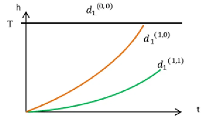
An example is shown on Figure 5 with the system defined in the previous method. This graph describes the

degradation function of 𝑃₁: 𝑑₁(1,1) being the normal degradation and 𝑑₁(1,0) the increased degradations, when the pump rotation speed is increased. Additionally, the function 𝑑1(0,0) represents the case where Z 𝜖 𝒵𝑓𝑓𝑓𝑓𝑓𝑓, that is to say

when ℎ_𝑖= 𝑇.

Figure 6 shows the process allowing calculating the 𝑅𝑅𝑅 on the previous example. Indeed, the indicator starts degrading following 𝑑₁(1,1), then when the system state changes (in this case a pump fails) it changes of degradation function and continues degrading following 𝑑₁(1,0) until the whole system fails.

C

S

It is important to note that the case study developed here aims to illustrate the method rather than demonstrate here, as it is not a real case.

System

Use—The system under study is a simplified bleed valve system. These valves are disposed in aircraft engines in order to regulate the bleed air pressure dispatched to downstream users. The valves can have several different positions and are moved by actuators.

Model— For the purpose of this paper, we consider that the system is composed by four identical valves. The valves are operating nominally when all four are functioning.

When one has a failure, the three remaining compensate the loss of air flow and thus function in “boost” mode, that is to say the demand in pressure from each valve will be higher and will therefore degrade faster. Finally when less than three valves are functioning, the system cannot fulfill its function with the required performance and is thus considered faulty.

Parameters— As described in part 3, the procedure takes in input a health state ℎ_𝑖 for each component and the different degradation functions 𝑑_𝑖 (that is to say every part 𝑑_𝑖𝑍 of each 𝑑_𝑖 function) for each component 𝐶_𝑖.

Since the purpose of this paper is to explain the method rather than how to obtain these parameters, they are considered known in this study. For the following of this case study and thanks to knowledge acquired on this system, we can define several spaces of which the system state 𝑍 can be a part. First: 𝓩𝒏𝒏𝒎𝒊𝒏𝒑𝒏= �� 𝟏 𝟏 𝟏 𝟏 �� (18)

is the space of the system states for which every component degrades nominally. Then: 𝓩𝒃𝒏𝒏𝒑𝒕= �� 𝟎 𝟏 𝟏 𝟏 � , � 𝟏 𝟎 𝟏 𝟏 � , � 𝟏 𝟏 𝟎 𝟏 � , � 𝟏 𝟏 𝟏 𝟎 �� (19) is the space containing the system states for which some components have an accelerated degradation due to some other components being faulty.

Finally:

𝓩𝒇𝒑𝒇𝒏𝒕𝒇= 𝓩 − 𝓩𝒏𝒏𝒎𝒊𝒏𝒑𝒏− 𝓩𝒃𝒏𝒏𝒑𝒕 (20)

Figure 6: Process For Changing Degradation Functions

Figure 7: Bleed Valve System Degraded Mode Modelling

Figure 8: Bleed Valve System Nominal Mode Modelling

V+

V+

V+

X

V

Is the space containing the states for which the system is faulty, as defined in the previous part.

Following these definitions, the valves degradation functions are showed on Figure 9, for valve 𝑖.

Study

The current time is 𝑇_𝑛𝐶𝑛. At this point, the value of the health indicators for the four components are known, and their evolution before this point is not important for the implementation of the method, as we just explained.

At the beginning of the study, in this case, the health indicator is below the threshold for each component, therefore they are all considered functioning nominally. The degradation functions associated to the normal degradation mode is therefore used to compute the 𝑅𝑅𝑅 for each component. This is showed on Figure 10.

At this point, we can note that the first method explained in part 2 would give 𝑆𝑅𝑅𝑅 = 𝑅𝑅𝑅₂ and the second one explained in part 3 would give 𝑆𝑅𝑅𝑅 = 𝑅𝑅𝑅₄.

The next step for the developed method is to select the minimal 𝑅𝑅𝑅, here 𝑅𝑅𝑅₂ . The “current” time is then updated to:

𝑻𝒏𝒏𝒏′= 𝑻𝒏𝒏𝒏+ 𝑹𝑹𝑹𝟐. (21)

Before 𝑇_𝑛𝐶𝑛′, the system’s state is � 1 1 1 1

�. After that date it

becomes � 1 0 1 1

� since the second valve has exceeded its 𝑅𝑅𝑅. Therefore after this point, the three other valves function - and therefore degrade - in “boost” mode.

According to the method developed in this paper, the components 𝑅𝑅𝑅 are recomputed after this point using the degradation functions linked to the right system state, that is to say the “boost” mode degradation for each component:

𝒅𝟏𝟐, 𝒅𝟑𝟐and 𝒅𝟒𝟐. (22)

Therefore 𝑅𝑅𝑅₁′, 𝑅𝑅𝑅₃′ and 𝑅𝑅𝑅₄′ are computed. This is showed on Figure 11.

Finally, since the condition for the system to work with the required performance is to have at least three valves functioning, the system 𝑅𝑅𝑅 is:

𝑺𝑹𝑹𝑹 = 𝑹𝑹𝑹𝟒′. (23)

This case study shows, on a simplified system, that the method developed in this paper can add accuracy compared to the methods previously explained. Moreover, taken the system reconfiguration into account will usually reduce the computed 𝑆𝑅𝑅𝑅 compared to the method taking only the system redundancy into account. Therefore it is a “safer” 𝑅𝑅𝑅 computing as it estimates a smaller 𝑆𝑅𝑅𝑅, while being closer to the real 𝑆𝑅𝑅𝑅.

Figure 9: Degradation Functions For The Bleed Valve System

Results

This system was implemented with the method explained, using arbitrary values. The health indicator values taken at 𝑇𝑛𝐶𝑛 are: 𝒉𝟏= 𝟎. 𝟒𝟒𝟒, (24) 𝒉𝟐= 𝟎. 𝟒𝟒𝟎, (25) 𝒉𝟑= 𝟎. 𝟑𝟒𝟎 (26) and: 𝒉𝟒= 𝟎. 𝟑𝟒𝟒. (27)

The nominal degradation function is computed thanks to a linear regression, using a history of each health indicator, and the “boosted” degradation function is taken constant, with a rate of 0.003 by flight cycle for the health indicators increase.

The 𝑆𝑅𝑅𝑅 is computed with each method. The first method, where the redundancy and system reconfigurations are not taken into account, returns:

𝑺𝑹𝑹𝑹 = 𝟒𝟎𝟎. (28)

The second one, which takes the redundancy into account but not the system reconfigurations, returns:

𝑺𝑹𝑹𝑹 = 𝟒𝟒𝟒. (29)

Finally, the method developed here returns: 𝑺𝑹𝑹𝑹 = 𝟒𝟑𝟐. (30)

These values illustrate the differences between each method. This case study showed several interests of the method developed in this paper.

First of all it showed that the computed 𝑅𝑅𝑅 for each component are more accurate than when computed separately. Indeed with this method the 𝑅𝑅𝑅 computed will always be equal or superior to the ones computed separately, therefore the components can be used longer without fear of unforeseen failures.

Then the real innovation of this method comes with the computing of an accurate 𝑆𝑅𝑅𝑅. This allows knowing when the system will stop completing its main function. The results of this case study confirm that this method is more accurate than when computing the component 𝑅𝑅𝑅 separately. It also confirms the importance of taking into account the system reconfigurations.

However this case study is based on a simple modelling of a real system, where the data such as the health indicators values and the degradation functions are given arbitrarily.

C

This paper introduced a new method allowing calculating a system-level 𝑅𝑅𝑅, and updating the components 𝑅𝑅𝑅 by using the system state. Therefore this a priori simple method takes into account not only the system redundancy, but also its reconfiguration, which tackles a new dimension in system-level prognostics. Although the assumptions are very simple, this adds a new level of precision into the 𝑆𝑅𝑅𝑅 computing compared to the most common methods which consist mostly in calculating the minimum between several component-level 𝑅𝑅𝑅. This method has already been implemented in python, with an architecture based on the OSA-CBM standard.

The second interest is that a complete model of the system or knowledge of its architecture are not needed for it to function. Only two things are needed as input for this platform, which are an initial health level for each component, and the degradation functions corresponding to each system state. This allows a great interoperability since the health levels and degradation functions can be supplied by different experts for different parts of the system, without the platform user knowing precisely where it comes from. The latter can then focus directly on the Health Management part, by using the 𝑆𝑅𝑅𝑅 provided by the platform.

The limitation of this method comes from the determination of these input parameters, which is not developed in this paper. Indeed, even though system experts could determine a useful health indicator, the degradation function can be

Figure 9: System-Level RUL Computing, Second Iteration

very complex to build for several reasons. First of all, even though the system functioning is usually very well known in the nominal mode, it is usually not the case for the degraded modes; therefore it could be hard to build degradation functions from system models in these modes. Then, proceeding to an offline data analysis to determinate the degradation functions can be useful in the nominal mode, but it could prove hard for the degraded modes. Indeed, a system will usually not stay long in these modes, either because it will be repaired or the system will go in a different degraded mode shortly after. Therefore, only a few data will be available in each degraded mode. Another advantage of this method, however, is that it leaves all possibilities to determine degradation functions open. In order to go further, it is therefore needed to obtain the input parameters. For that, two different approaches are available. The first one relies only on data mining, and an offline analysis of recorded data on the systems. However, for the reasons explained just above, it could take a long time before enough data are gathered on systems to use them. The second solution is to take into account Prognostics and Health Management from the beginning of the system design phase. It consists in building useful indicators, place sensors to measure the needed variables, and being able to transmit this information to a health management system.

R

[1] Andrew. K.S. Jardine, Daming Lin, and Dragan Banjevic. A review on machinery diagnostics and prognostics implementing condition-based maintenance. Mechanical Systems and Signal Processing, 20(7): 1483 – 1510, 2006.

[2] A. Heng, S. Zhang, Andy C.C. Tan, and J. Mathew. Rotating machinery prognostics : State of the art, challenges and opportunities. Mechanical Systems and Signal Processing, 23(3): 724 – 739, 2009.

[3] J.Z. Sikorska, M Hodkiewicz, and L Ma. Prognostic modelling options for remaining useful life estimation by industry. Mechanical Systems and Signal Processing, 25(5): 1803–1836, 2011.

[4] Venkat Venkatasubramanian. Prognostic and diagnostic monitoring of complex systems for product lifecycle management : Challenges and opportunities. Computers & Chemical Engineering, 29(6): 1253 – 1263, 2005

[5] A. Soualhi, K. Medjaher, N. Zerhouni. Bearing Health monitoring based on Hilbert-Huang Transform, Support Vector Machine and Regression. IEEE Transactions on Instrumentation and Measurement, vol.64, no.1, pp.52-62, Jan. 2015 doi : 10.1109/TIM.2014.2330494.

[6] A. Mosallam, K. Medjaher, N. Zerhouni. Data-driven prognostic method based on Bayesian approaches for direct

remaining useful life prediction. Journal of Intelligent Manufacturing, article published online 13 June 2014, DOI : 10.1007/s10845-014-0933-4.

[7] K. Medjaher, D.A. Tobon-Mejia, N. Zerhouni. Remaining useful life estimation of critical components with application to bearings. IEEE Transactions on Reliability, vol. 61, no. 2, pp. 292-302, 2012

[8] D.A. Tobon-Mejia and K. Medjaher and N. Zerhouni. CNC machine tool’s wear diagnostic and prognostic by using dynamic Bayesian networks. Mechanical Systems and Signal Processing, vol. 28, pages : 167 - 182, DOI : 10.1016/j.ymssp.2011.10.018, ISSN : 0888-3270, 2012 [9] H. Skima, K. Medjaher, C. Varnier, E. Dedu, J. Bourgeois. Hybrid prognostic approach for Micro-Electro-Mechanical Systems. 2015 IEEE Aerospace Conference, March 2015, Big Sky, Montana, USA.

[10] Xavier Desforges, Mickaël Diévart, Philippe Charbonnaud, Bernard Archimède. A distributed Architecture to implement a Prognostic Function for Complex Systems. First European Conference of the Prognostics and Health Management Society, Dresden, Germany, 3-5 July 2012, ISBN: 978-1-936263-04-2

[11] Chaochao Chen, Douglas Brown, Chris Sconyers, Bin Zhang, George Vachtsevanos, Marcos E. Orchard. An integrated architecture for fault diagnosis and failure prognosis of complex engineering systems. Expert Systems with Applications, vol. 39, Issue 10, August 2012, Pages 9031–9040

[12] Manzar Abbas, George Vachtsevanos. A System-Level Approach to Fault Progression Analysis in Complex Engineering Systems. Annual Conference of the Prognostics and Health Management Society, San Diego, CA September 27 – October 1, 2009, ISBN: 978-1-936263-00-4

[13] Peysson Flavien, Mustapha Ouladsine, Rachid Outbib. Complex System Prognostics : a New Systemic Approach. Annual Conference of the Prognostics and Health Management Society, San Diego, CA September 27 – October 1, 2009, ISBN: 978-1-936263-00-4

[14] W. ElGhazel , A. Farhat, J. Bahi, C. Guyeux, M. Hakem, K. Medjaher, N. Zerhouni. Random Forests for Industrial Device Functioning Diagnostics Using Wireless Sensor Networks. 2015 IEEE Aerospace Conference, March 2015, Big Sky, Montana, USA.

B

Josselin Maitre got an Ingénieur diploma from Ecole Nationale Supérieur de Mécanique et des Microtechniques of Besançon in 2015. He is an aviation enthusiast and interested in complex systems. He did an internship at Liebherr Aerospace Lindenberg where he discovered the aeronautic industry and one at Airbus Group Innovations where he discovered PHM and its application to systems failure prediction. He is now studying an Advanced Master in Systems Engineering at ISAE-SUPAERO aiming designing complex systems while keeping in mind PHM.

Jayant Sen gupta (Ingénieur Ecole Polytechnique (2000), PhD in Computational Mechanics, Ecole Normal

Supérieure de Cachan (2005)) has been a research engineer at Airbus Group Innovations since 2005. His topics of interests moved progressively from HPC for computational mechanics to uncertainty modeling and propagation in physical models. Since 2009, he has been involved in the development of Prognostics and Health Management in Airbus Group. He has developed the PHM function that monitors A380 and A350 fleets through AiRTHM, the real time health monitoring service of Airbus. His activities mainly focus now on data analysis to extract relevant health indicators from operational data.

Kamal Medjaher received the M.S. degree in control and industrial computing from the University of Lille 1, Villeneuve-d’Ascq, France, and Ecole Centrale de Lille, Villeneuve-d’Ascq, in 2002, and the Ph.D. degree in control and industrial computing from the University of Lille 1, in 2005. He has been an Associate Professor with the National Institute in Mechanics and Microtechnologies, Besançon, France, since 2006. His teaching activities concern control systems, fault detection, fault diagnostics, and fault prognostics. His current research interests include prognostics and health management (PHM) with special developments in data processing, feature extraction, degradation modeling, health assessment, and remaining useful life prediction.

Noureddine Zerhouni received the Engineering degree from the National Engineers and Technicians Institute of Algiers, Algiers, Algeria, in 1985, and the Ph.D. degree in automatic control from the Grenoble National Polytechnic Institute, Grenoble, France, in 1991. He joined the National Engineering Institute of Belfort, Belfort, France, as an Associate Professor in 1991. Since 1999, he has been a Full Professor with the National Institute in Mechanics and Microtechnologies, Besançon, France. He is a member of the Department of Automatic Control and Micro-Mechatronic Systems at the FEMTO-ST Institute, Besançon. He has been involved in various European and national projects on intelligent maintenance systems. His current research interests include intelligent maintenance, and prognostics and health management.