Do school-going children with more active modes of morning commutes walk more throughout the day?

Do school-going children with more active modes of morning commutes walk more throughout the day?

By

Shin Bin Tan

B.A in Sociology

Wellesley College (2007)

Submitted to the Department of Urban Studies and Planning

in partial fulfillment of the requirements for the degree of

Master in City Planning

at the

MASSACHUSETTS INSTITUTE OF TECHNOLOGY

February 2017

© 2017 Shin Bin Tan. All Rights Reserved

The author here by grants to MIT the permission to reproduce and to distribute publicly paper

and electronic copies of the thesis document in whole or in part in any medium now known or

hereafter created.

Author_________________________________________________________________

Department of Urban Studies and Planning

17 January 2017

Certified by _____________________________________________________________

Assistant Professor Mariana Arcaya

Department of Urban Studies and Planning

Thesis Supervisor

Accepted by______________________________________________________________

Associate Professor P. Christopher Zegras

Chair, MCP Committee

Department of Urban Studies and Planning

Do school-going children with more active modes of morning commutes walk more throughout the day?

by Shin Bin Tan

Submitted to the Department of Urban Studies and Planning, Feb 2017, in partial fulfillment of the requirements for the degree of

Master in City Planning

ABSTRACT

Boosting physical activity in school-going children has multiple health and educational benefits. One strategy to boost physical activity is to have students adopt more active commutes. However, empirical health studies suggest that students respond to physical activity interventions by cutting down their activity throughout the rest of the day. If such compensatory behavior occurs in response to commuting-based physical activity initiatives, then these initiatives may not achieve their desired outcomes.

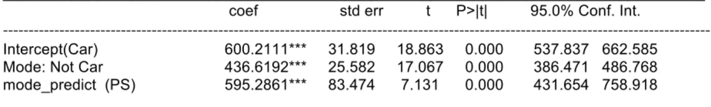
Using a dataset of walking data logged by about 7,700 Singaporean students wearing portable sensors, I examine the question: Do students who walk or take public transport to school walk more throughout the day than their peers who are driven to school, or do they compensate for more active morning commutes by walking less for rest of the day? This study triangulates three statistical approaches to identify the relationship between morning commute mode choice and walking activity: a multivariate linear regression model that includes potential confounders like students’ age group, household socio-economic status and built environment characteristics around home and school; a propensity score covariate adjustment model using similar baseline covariates as the first analysis; and a fixed effects model that estimates the net impact of inter-day mode changes for each individual student. Results from all three analyses suggest that students who take public transport or walk to school log a statistically significant and substantial number of steps more than their counterparts who are driven to school. However, this positive difference is whittled away by the end of the day, which supports the hypothesis that students with more active commutes compensate by walking less throughout the day. Programs to encourage active commuting may thus have limited effectiveness in boosting students’ physical activity

ACKNOWLEDGEMENTS

Professor Mariana Arcaya: Thank you for being a great advisor, a fount of statistical

knowledge and an all-round source of inspiration.

Professor Chris Zegras: Thank you for being an enthusiastic, supportive reader, and

for constantly pushing this study and me in new directions.

Family and friends: Thanks for being there for me, whether in person or over the

phone. Special thanks goes to David L. for reviewing my thesis and for being a solid

cheerleader throughout.

DUSP classmates: It has been an honor meeting and learning with a group of

passionate, driven individuals. I will miss the camaraderie.

Daosong: All the rest of my thanks go to my husband who endured many rambling,

highly suspicious-sounding conversations about tracking where children go, and who

nevertheless remained unflappably supportive throughout.

CONTENT PAGE

I. Introduction to Research Question 6

a. Study’s Objectives 6

b. Scope of Study and Organization 9

II. Theoretical Framework and Literature Review 10

a. Theories of Behavioral Regulation and Setpoints 11

b. Existing Research on Active Commuting & Activity Setpoints 12

c. Other Factors that Affect Walking Activity Other than Mode Choice 14

III. Data and Methods 18

a. Overview of NSE Data and Study Context 18

b. Defining Model Variables 19

c. Data Filtering Procedures 31

IV. Analysis Results 34

a. Descriptive Statistics 34

b. Analysis and Findings 36

c. Sensitivity Analyses 51

V. Discussion 57

a. Results, Discussion and Policy Recommendations 57

b. Limitations and Further Studies 59

VI References 62

I.

Introduction to Research Question

a. Study’s Objectives

Early each weekday morning, approximately half a million Singaporean students embark on their journey to school (Department of Statistics, 2016). How each student travels to school can affect the amount of physical activity a student starts his or her day with. For students who walk to school, or who walk to and from transit stops when taking public transport to school, this morning commute represents their first physical exertion of the day. For others, their morning commute involves passively sitting in the comfort of a car or private bus shuttle, as they are driven directly from home to school.

One may expect that students who walk more as part of their morning commute accumulate more steps throughout the day compared to their counterparts who do not have such active commutes. However, some studies suggest individuals regulate their physical activity in order to maintain a certain budget or ‘set-point’ of activity. If so, one would then expect that students who have more active commutes may end up compensating for their morning activity by walking less throughout the rest of the day.

This study assesses whether encouraging students to walk or take public transport to school instead of being driven can be an effective way to boost overall walking activity, or whether students end up compensating for more active morning commutes by walking less throughout their day. The extent to which students’ choice of morning commute mode contribute to their overall walking is an important one to understand for the following three reasons:

i. Active Commuting As Exercise

Obesity is a growing problem in many developed countries. For instance, in the US, the problem of obesity is severe, with an estimated 32% of youths (ages 2-19) overweight or obese, as of 2012 (Ogden et al, 2014). While obesity rates in Singapore are not as high as in the U.S, there has been an upward tick in the prevalence of being overweight/ severely overweight.

For example, the prevalence of overweight and severely overweight was only 1.4% for Primary 1 (ages 6-7) students in 1976, which has increased to 12.7% by 2006. For school

children in mainstream schools from primary to pre-university levels, the overweight and severely overweight prevalence was estimated to be 11% in 2011 (Foo et.al, 2013).

Boosting physical activity is one way to tackle this obesity challenge. (Janssen & LeBlanc, 2009) Unsurprisingly, studies indicate that many children, both in the United States and Singapore, are not meeting national recommendations of having 60 minutes of daily physical activity. In the U.S, according to the National Youth Risk Behavior Survey 2015 survey of 9th to 12th graders, less than half of respondents reported that they were physically active for at least 60 minutes on 5 or more days a week. (CDC, 2015) According to a 2012 Students’ Health Survey in Singapore, only 16% of students aged 13 to 16 years old were physically active for at least 60 minutes on five or more days a week (Health Promotion Board Singapore, 2012).

There have been various efforts to boost physical activity amongst school-going children in Singapore. For instance in 1992, the Ministry of Education introduced the Trim and Fit (TAF) Program in Singapore’s schools, where overweight students were required to participate in special physical activity programs. The program was reviewed and replaced, after concerns about the stigma associated with participation in TAF were raised (Foo et.al 2013). Currently, schools in Singapore adhere to a ‘Holistic Health Framework’, which, according to the Ministry

of Education, was “introduced to broaden health promotion of schools beyond obesity and

fitness management by embracing the total well-being for student and developing their intrinsic motivation to lead a healthy lifestyle” (Ministry of Education Singapore, 2016).

One strategy to boost physical activity that schools in the U.S, U.K and Australia have experimented with is active commuting initiatives, such as ‘walking school buses’ where students walk to school in a group while supervised by an adult, or ‘walk to school days’, where a day out of a week would be assigned for students to walk to school (Chillon et.al, 2011).

Another way to boost walking is by encouraging students to take public transport to school, rather than be driven. Taking public transport can increase an individual's level of physical activity because of the need to walk or bike at the beginning and end of each trip (Sener et. al, 2016). For instance, a 2013 study that surveyed students and staff at the University of Sydney, Australia, found that those who used public transit or active modes for school

commutes reported an average of 174 minutes of physical activity per week, compared to 115 minutes for drivers (Risseletal, 2013 ).

As Singapore has an extensive public transportation system and a tropical clime that does not get too cold for walking, encouraging students to switch from being driven to taking public transport or walking to school could be a viable strategy to boost their daily steps. Furthermore, younger primary school students tend to live within walking distance to schools because of policies that prioritizes the allocation of school places to students living within a one kilometer of the school first, then students within 2 kilometers next. Effectively, if demand by families living within a two kilometer radius from the school exceeds the total available places the school offers, students living outside this radius would not be admitted, unless they have additional affiliation with the school that can boost their chances of admission. (Agarwal et. al, 2016).

Establishing how much active commutes add to overall activity can help policy-makers better understand the likely effectiveness of initiatives promoting active morning commutes in increasing overall physical activity. Furthermore, a better understanding about what factors affect walking (whether they be built environment measures, or socio-economic influences) can enable policy-makers to tailor their programs to encourage more overall physical activity.

ii. Active Commutes to improve education outcomes

In additional to health benefits, physical activity has been associated with better academic

performance. A 2011 review of the scientific literature that examined the association between

school based physical activity (physical education, recess time, in-class physical activity and extra-curriculars) and academic performance (including indicators of cognitive skills and attitudes, academic behaviors, and academic achievement) found substantial evidence that physical activity could help improve academic achievement (Raspberry et. al, 2011).

Several studies observed that students who had opportunities be active, such as recess breaks, were less fidgety, and more focused and on-task post-activity (Mahar et.al 2006 ;

Jarrett et.al 1998)/ Similarly, an experimental study carried in 2013-2014 on 77 third and

fourth-graders in two US schools found that before-school walking/running programs helped enhance class-room on-task behavior (Stylianou et. al, 2016). These findings suggest that

physical activity before class could potentially improve in-class focus by reducing ‘activeness’ within the classroom.

A small number of studies examine the cognitive impact of active commutes. Two of these, one conducted in Spain (Van Dijk et.al 2014) and the other in Holland (Martinez –Gomez et.al, 2011) suggest that active commuting to school is positively associated with cognitive performance or attention for girls but not for boys. Another project, “The Mass Experiment 2012” which involved 20,000 Danish children from the ages of 5 to 19 found that those who walked or cycled to school rather than driven performed better on a concentration test (Vinther, 2012) (HASTE, 2013). However, limited information about this project is available, since it was set up primarily as a learning program for school children rather than an actual research study. Nevertheless, the study has captured some public interest (Goodyear, 2013). From an educational and learning outcomes perspective, a better understanding of the impact of walking during a child’s morning commute on his or her subsequent ‘activeness’ for the rest of the school day could be valuable for educators as it could provide insights about the scheduling of physical activity during school hours, or help persuade parents and students to opt for more active commutes.

iii. Encouraging walking as environmentally sustainable travel

From a transportation perspective, both walking and use of public transport are generally seen as a preferred mode choice compared to driving, which has many negative externalities such as increasing both congestion and carbon emissions (Litman, 2009). There is thus much interest in ways to encourage people to walk or take public transport.

However, if individuals adhere to a set budget for walking, efforts to shift people from one mode to the next would have to take these constraints into consideration. Understanding whether there is a ‘budget’ or set-point that people have for walking could thus help transportation experts and policy-makers formulate more realistically effective walking policies.

b. Scope of Study and Organization

The remainder of this thesis is organized as follows: Section Two provides an overview of different theories of behavioral regulation and set points that form the theoretical framework

for this thesis, as well as existing empirical research on the effectiveness of physical activity interventions and active commuting strategies. This section also summarizes existing research on factors that influence the amount of walking one does. Section Three describes the data used in the study, and how this data was filtered and processed for further analysis, while Section Four covers the study’s analyses and findings. The last section, Section Five, concludes with a discussion of the implications of the study results, limitations and recommendations for further research.

II.

Theoretical Framework and Literature Review

a. Theories of behavioral regulation and set points

Theories about certain ‘setpoints’ or ‘budgets’ constraining human behavior span different fields.

Health: Health literature posits the idea of a weight ‘set-point’ where the human body has a ‘feedback control system’ that regulates body weight by adjusting food intake, energy expenditure or both in proportion to the difference between current body weight and the ‘set point’ weight (Muller, Bosy-Westphal & Heymsfield, 2010). The set-point model has also been applied more specifically to activity regulation. The ‘activitystat’ model posits that when an individual increases his or her physical activity or energy expenditure in one domain, there is a compensatory change in another domain, in order to maintain an overall stable level of

physical activity or energy expenditure (Gomersall et al, 2016).

Transport: The concept of a “travel time budget” is well-established in transport literature. This theory hypothesizes that one’s average daily travel time tends to be relatively constant, and that each individual has a budgeted amount of time they are willing to spend on travelling and would adjust their choices to keep to this budget. For instance, improvements in technology or additional capacity that create faster travelling speeds are seen to lead to longer travel distances, while travel times remain relatively constant (Mokhatarian et. al 2004).

There has been some limited research that suggests that the existence of a ‘walking’ budget. A 2007 study of the Twin Cities observed that dense areas promote travel walking while less connected areas promote leisure walking, and that the two effects seem to counterbalance each other so that total walking and physical activity are not affected by either (Oakes et al, 2007). Similarly, a 2006 study compared a large ‘new-urbanist’ neighborhood with conventional suburban neighborhoods, and found no significant difference in overall physical activity between residents of either neighborhood types. However, residents in the urbanist neighborhood tended to walk more within their neighborhood for utilitarian travel and less elsewhere for leisure, suggesting that utilitarian travel substitutes for other physical activity

(Rodriguez et al, 2006). Collectively, these two studies have been interpreted to suggest a physical activity budget that constrains walking (Krizek, Handy & Forsyth, 2009).

One could hypothesize that a ‘total daily steps’ budget exists for students, possibly because

they are self-regulating their energy expenditure, as suggested by the activity-stat literature, or because they have a limited amount of time for walking, as suggested by the transportation literature. If such a setpoint exists, we could expect students who are relatively more active during commuting hours to dial back on their walking for the rest of the day, and for commuting modes to thus have little or no perceptible net impact on overall activity.

b. Existing research on active commuting & activity setpoints

i. Effectiveness of Active Commuting Interventions

Most studies that focus on the impact of active commuting strategies, such as walking school buses, find that active commuters tend to have greater overall physical activity over the day. A review of studies from 2008-2012 that looked at children of school-going ages (5 to 17.9 years old), and that have assessed daily physical activity level through objective measures (e.g. pedometers) or subjective measures (surveys), body composition variables (BMI, waist circumference, skinfolds, etc.), and/ or cardiovascular fitness was published in 2014. This review found consensus among many of these studies that active school transport leads to more moderate-vigorous physical activity (MVPA) over the course of the day (Larouche et. al, 2014).

49 of the reviewed studies focused on Active School Transport (AST) and daily physical activity. Of the 28 studies used accelerometers to measure physical activity, 22 concluded that AST was associated with higher physical activity levels. Several studies also found that the difference in physical activity between active and passive travelers often exceeded the amount associated with the journey to and from school. This suggests that the more active commuters accumulated more MVPA than can be attributed to their commutes. Similarly, 8 out of 9 studies that used pedometers to track steps found that AST was associated with higher daily step counts, ranging from an average of 663 to 3477 more steps per day.

An earlier review of studies on the impact of active school transport, and which included an objective measure of physical activity such as pedometers or accelerometers came to similar conclusions (Faulkner and Edward, 2009) came to similar conclusions. Of the 13 studies examined, 11 found that children and youth who were active school commuters were more physically active than those who took motorized transport. Four studies found at least a 20-minute difference in daily MVPA between active and passive school commuters. This 2009 review also highlighted that studies examining physical activity patterns on the weekend consistently revealed no significant difference in activity levels between active and non-active school commuters on weekends. The observation that active school commuters were not more inclined towards being physically active provides some evidence against self-selection as an explanation for higher levels of physical activity among active school commuters. (Cooper et. al., 2003, Cooper et. al. 2005; Sirard et al., 2005, Duncan et al., 2008).

In contrast, a recent 2015 review of 12 studies on the impact of walking school buses found more mixed results(Smith et. al 2015). Of the three RCTs that were included in the review, two RCTs suggest that such programs did not affect general activity levels in sizeable or significant ways. For instance, one found that those in the intervention group had only a 2 minute increase in moderate-to-vigorous activity (MVPA) from their baseline, and 7 minutes more of MVPA compared to the control group (Mendoza et. al, 2011) while the another RCT found no difference in total daily activity between groups that participated and those that did not—this was however attributed to insufficient power to detect differences because of the high variability of physical activity behavior and measurement error (Sirad et. al, 2008).

ii. Effectiveness of General Physical Activity Interventions

Compared to studies specifically on active commuting, studies on the effectiveness of physical activity interventions in boosting students’ activity levels are less in agreement.

A meta-review of 30 studies on children aged 16 or younger that tested the effectiveness of interventions to boost physical activity, including school-based physical activity programs and active video games, was published in 2012. This meta-review, which comprised 27 Randomized Controlled Trials studies and three controlled clinical trials, found that the intervention effect was minimal (small to negligible) for total physical activity. This review found strong evidence that physical activity interventions had only small effects (approximately 4 minutes more walking or running per day) on children’s overall activity levels,

and from there extrapolated that the small effect explained why interventions had limited success in reducing the children’s body mass index or body fat (Metcalf et al, 2012). While the meta-review did not focus on examining compensatory effects of interventions, one explanation it offered for the lack of success of physical activity interventions was that children might have been compensating for imposed increased activity.

Several studies that did focus specifically on testing whether there was physical activity compensation among children yielded mixed findings. A 2000 study that used accelerometers to track 76 third and fourth-graders’ activity over four days, found that students did not compensate for a sedentary school day by increasing their levels of physical activity after school. (Dale et. al, 2000) . In contrast, a 2003 UK study which used accelerometers to measure the physical activity of 215 children ages 7 to 10.5 found that students from one school with extensive sporting facilities and 9 hours of scheduled physical education a week did about the same amount of physical activity as students from two other schools with less than 3 hours of scheduled physical education. The study’s authors thus concluded that the total amount of physical activity done by the students did not depend on the amount of physical education timetabled because students compensated for school physical activity when out of school (Mallam et.al, 2003).

There thus seems to be some divergence in studies whether school-going children keep to a budget of activity throughout the course of a day.

c. Other factors that affect walking activity other than mode choice

Mode of travel is one out of many factors that could influence the number steps students take. Any analyses of the relationship between mode and walking activity should thus include consideration of such factors linked to walking behavior. The following paragraphs explore these factors in greater detail.

i. Age and Gender:

Various studies show that older children generally take fewer steps than their younger counterparts, and their step counts decrease throughout adolescence. Girls also tend to walk less than boys. (Tudor-Locke et. al 2011; Barreira et.al, 2015)

ii. Built Environment Characteristics:

The built environment can also influence an individual’s walking behavior, because it affects the number, type and quality of different activities, locational distribution of these activities and thus travel distances and the relative travel costs that may encourage or discourage walking. (Frank and Engelke, 2001).

While there are many different ways of categorizing and describing the built environment, commonly used built environment categories and their hypothesized link to walking are as follows (Ewing & Cervero, 2010):

● Density: As its name suggests, built environment density refers to the amount of a variable of interest, such as population, dwelling units, employment, or building floor area, per unit area. Increased density helps shorten distances between activities, which facilitates walking. Density also affects the subjective experience of walking— contributing a sense of liveliness or crowding (Lawrence & Engelke, 2001).

● Diversity: This refers to the number of different land uses, like housing, retail, and office, in a given area. Measures of landuse diversity include entropy measures of diversity, jobs-to-housing or jobs-to-population ratios. Higher landuse diversity is theoretically linked with more walking, since having a variety of different uses within shorter, walkable distances allow more opportunities to link different trips by foot (Cervero & Kockleman, 1997). Mixed land uses are also believed to help reinforce streets as public spaces, create a sense of community and local investment, and could potentially help enliven the walking experience.

● Design: Street network characteristics, such as block sizes, proportion of four-way intersections, sidewalk coverage, average building setbacks, average street widths and number of pedestrian crossings, collectively capture the design aspect of an urban environment.

Certain design schemes, such as siting store entrances near curbsides and parking in the rear, help make destinations more accessible and conveniently reached by foot.(Cervero & Kockelman, 1997). Furthermore, pedestrians, compared to motorists,

move relatively slowly through the urban environment, and can pick up more detailed nuances of the street-level environment. Streets that offer visual and sensory contrasts, and which have ample sidewalks and slower, less threatening traffic are thus more appealing for walking (Lawrence & Engelke, 2001).

● Destination accessibility: This refers to the ease of access to ‘attractions’ or ‘destinations’ such as employment centers, shopping areas or retail outlets. Neighborhoods with more destinations that are accessible by foot are more likely to attract people to walk to, and to explore by foot.

● Distance to transit/ accessibility to public transport: Areas can be characterized by their proximity to transit stations or bus-stops, or how many transit stops are available per unit area. Theoretically, better accessibility to transit options should encourage greater use of public transport, which has been linked to more walking. The empirical link between the built environment and its impact on travelling behavior, including walking as a mode of transport, has been studied extensively, and there have been multiple meta-reviews of existing research. One of the more recent reviews (Ewing & Cervero, 2010) found walking to be most strongly related to land use diversity, intersection density and number of destinations within walking distance, whereas bus and train use is more related to proximity to transit and street network design variables, with land-use diversity being a secondary factor. Overall, the review concluded that travel behaviors are generally inelastic with respect to change in individual measures of the built environment. However, the combined effects of several variables may be sizeable, which suggests that the built environment measures should be studied together as a combined package, rather than in an isolated manner.

Besides studies on the built environment that examine adult walking behavior, there have also been some specific to a younger population. These studies suggest that, while what constitutes a walkable environment for adolescents is largely similar to that of adults, there are several notable differences. For instance, density and street design of the home environment—aspects significantly associated with adult walking—have been less consistently associated with adolescents’ physical activity. Rather, adolescent walking is more

consistently associated with the proximity of parks and other facilities that support physical activity (Rodriguez et. al 2015).

More specifically, students’ propensity to walk to school is negatively associated with distance to school, and positively associated with population density, high land use diversity, and a pedestrian oriented street design around both home and school (Rodriguez et. al 2015). Collectively, the literature suggests that the built environment is likely to have a significant impact on walking in general, for both adults and children.

iii. Socioeconomic Status

Individuals’ thresholds for walking have been shown to vary according to their socio-economic (SES) characteristics. A 2016 study based on data from over 8,800 adults in Brisbane, Australia found that full-time high income earners and part-time workers seem most sensitive to walking time, whereas young adults who are both working and in school are the least sensitive to walking times when choosing their travel mode (Lee and Kamruzzaman, 2016). Other studies have found that residents in low SES neighborhoods were less physically active compared to those in high SES neighborhoods. For instance, a recent 2015 Australian study examined whether the associations between recreational walking and environmental attributes such as residential density and intersection density were moderated by area-level SES. The study’s researchers concluded that, consistent with other studies that found walkability associated with walking regardless of SES levels, the link they found between environmental attributes and recreational walking were largely similar for low and high SES areas. However, they did find residential density being associated with walking specifically in low SES areas only, suggesting some evidence of built environment modification by neighborhood SES (Takemi et. al, 2015).

III. Data and Methods

a. Overview of NSE Data and Study Context

Between September to November 2015, a ‘National Science Experiment’ (NSE) was initiated by the Singapore Ministry of Education in partnership with the Singapore University of Technology and Design (SUTD), Science Centre Singapore (SCS), Agency for Science, Technology and Research (A*STAR), Singapore Land Authority (SLA). As part of the NSE, approximately 50,000 lightweight SENSg devices developed by SUTD were deployed to school children from different levels --Primary (ages 7 to 12), Secondary (ages 13 to 16) and Junior College (ages 17 and 18), across 128 schools. The intention of the NSE was to spark interest in science and engineering in students by giving them their own data to analyze. These SENSg devices (Fig 3.1) included several different sensors that collected information about temperature, light, humidity, noise, motion, and Wi-Fi access points. Sensor nodes that were moved within the past five minutes would log all sensors at 10 seconds intervals, and poll motion data at one second intervals. The sensors used Wi-Fi signals to identify the location of its user. MEMS accelerometers included in the SENSg device measured the magnitude of acceleration and used this to compute each user’s step counts throughout the day. However, the pedometer function included in the device alone was occasionally not sensitive enough to capture small periods of walking (e.g. when boarding a bus). Step numbers should thus to be considered as an indication of how much walking a students does rather than an absolute, accurate measure, since the step count depended on how the sensor was worn, and on the gait of individual students (Wilhelm et. al, 2016).

Students were given instructions not to carry their devices when doing vigorous activity, such as sports or during Physical Education classes. The number of steps picked up by the SENSg device are thus likely to be ones that are more or less purely walking, and are not a good direct measure of overall physical activity.

Fig 3.1: Students with SENsg sensors1

Morning Commute Mode

(Car, PT, Walk) Total Daily Steps

Family Income

School Built Environment Home Built Environment Age

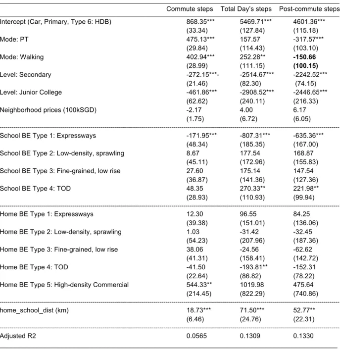
b. Defining Model Variables

In this study, the main outcome variable of interest is the total number of steps students took, while the main predictor variable is their morning commute mode.

At the same time, there may be several other confounders that could affect a student’s choice of mode and their total steps, which have to be included into the analysis. (Fig 3.2) For example, younger students may more likely be driven, compared to older students, because their parents may be less willing to let them brave the commute to school alone on public transport. Given the extremely high prices of cars in Singapore, students from wealthier families are also more to have access to a car, and thus more likely to be driven. As one’s SES may also have an impact the number of steps one takes, SES could be another confounder. Furthermore, built environment and characteristics may influence students’ morning commuting mode—for instance, students who live in neighborhoods with poor pedestrian connectivity and access to public transit may be more likely to be driven to school, and may also walk less because of the less attractive pedestrian experience they have at home.

Fig 3.2: Diagram showing relationship between morning commute mode and steps

Details of the model analysis will be covered in greater detail in the subsequent section of this paper, while the following paragraphs describe the variables included in the study.

A combination of Python libraries, R2_{and R packages, and open-source geospatial software}

QGIS3 _{were used to process the NSE sensor data and calculate the following variables for} analysis.

2 _{R Core Team (2016). R: A language and environment for statistical computing. R}

Foundation for Statistical Computing, Vienna, Austria. URL https://www.R-project.org/.

3 _{QGIS Development Team, 2009. QGIS Geographic Information System. Open Source Geospatial Foundation. URL}

i. Step Count:

The main outcome variable for the study is the total number of steps students took within 24 hours of a day (12 midnight to 11.59PM). This measure is further broken down into two time frames: the first spans 4am to 8am, which represents the window where students were likely

to be commuting to school4. The second time period covers the rest of the day from 8am till

midnight. Steps taken within the first time period are referred to as ‘commute steps’ while steps taken in the second time period are referred to as ‘post-commute steps’ henceforth. The purpose of analyzing commute and post-commute steps separately from total day’s steps is to ascertain how mode choice affected walking within each time period, and from there deduce whether students compensated for more steps taken as part of their commute during the time after their commutes.

ii. Morning Commute Mode:

The main predictor variable is the mode of morning commute. SUTD researchers ran various trip-detection algorithms on the students’ morning trips, to ascertain the likely mode taken. For each student, his/her recorded trip was compared to all possible routes based on Google Maps Direction API, for different transportation choices. The most ‘geographically similar’ match would be picked, and further checked against preset thresholds of travel duration, distances and geographical similarity. If these thresholds were satisfactorily met, this travel mode would be assigned to the student’s morning trip (Wilhelm et. al 2016).

While this method of mode-matching worked reasonably well for vehicle trips, it did not work as well for short walking trips because of the sensor’s Wi-Fi-based localization technology was not sufficiently accurate. SUTD researchers thus recommended using an alternative method

of mode identification specifically for walking trips5_{, which was based on the sensors’}

pedometer readings, combined with light and humidity readings to detect whether the student is indoors or outdoors (Wilhelm et. al 2016). The two methods of mode-deduction were combined.

iii. Age

The NSE dataset included the name of each participant’s school. Based on the school name, one could infer whether the school was a primary school (7-12), secondary school(13-16) or

junior college(17-18), and therefore what broad age group the student belonged to. Each participant’s school level was thus used as a proxy for their age.

iv. Home - School Distance

As the distance between a student’s home and school location determines how far he/she has to travel in the morning, which may affect total commuting steps taken, another control variable included in the analysis was the distance between each student’s home location and school location.

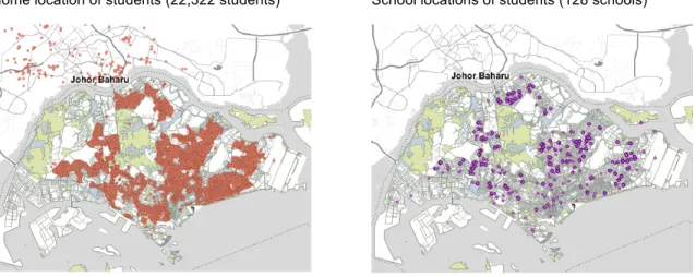
SUTD researchers had previously estimated likely home and school locations from each day of data records by identifying clusters of aggregated location coordinates (Wilhem et. al, 2016). This study uses these identified home and school locations as a starting point, (Figure 3.3) and calculated the straight-line distance between each student’s home and school.

v. Neighborhood Property Prices as a proxy for household SES

The NSE sensor data did not include any additional information about each student, besides their locations and school names. As a proxy for each student’s household economic status, a neighborhood average of recent property transactions was calculated.

Broadly speaking, Singapore’s owner-occupied housing market consists of two separate parts: a resale market of subsidized public flats built by Housing Development Board (HDB) and private residential property market (Tu and Wong, 2002).

Figure 3.3: Home and School locations of study participants

The majority of Singapore residents live in public HDB flats. According to Singapore’s 2015 General Household Survey (GHS)—where 33,000 respondents were selected from a sampling frame comprising all residential dwelling units in Singapore—about 80% of residents in Singapore currently live in HDB flats (Department of Statistics, 2015). These flats, offered on a 99 year leasehold, can be bought and sold on a resale market.

Private property transaction data dating from August 2013 to July 2016 was obtained from the

Urban Redevelopment Authority’s website6_{, while resale public housing flat transaction prices}

from between March 2012 to June 2016 were downloaded from data.gov.sg. New HDB flat prices were not included in this analysis for several reasons. Firstly, as new flats tend to be allocated to young, newly married couples, most buyers of new flats within time period (2013 to 2016) used here to construct the property price layer are less likely to have a child of school-going age. Thus, using a measure of transaction prices of resale flats would likely be more representative of the household income of students participating in this study than a measure that included new flat sales.

Furthermore, government policies, rather than the market, determine sales prices of new flats. The government sets the sales price of new HDB flats, building in subsidies into these prices. Generous additional housing grants of up 80,000 SGD (or approximately 56,000 USD) are also offered to eligible households that fall below set income thresholds, which further offset

the listed flat prices.7 _{All in all, one could argue that the sale prices of new HDB flats are not}

good reflection of a household’s income, especially when considered together with either resale flats sold on the open market, or private housing. Adding new flat sales may be particularly distortionary, as these are usually transacted in bulk, and would likely substantially pull down the mean of overall neighborhood prices.

Transaction prices for private property and resale public housing were then adjusted by their

respective quarterly price indices8 _{to a common base quarter of 2013Q2. The listed}

transactions of private landed housing units included street names, condominum sales included the project name, and public housing resale transactions included the exact block

6 _{URA, “Private Residential Property Transactions”, https://www.ura.gov.sg/realEstateIIWeb/transaction/search.action. Accessed}

August 2016.

7 _{Housing Development Board Singapore, “HDB Flat”, http://www.hdb.gov.sg/cs/infoweb/residential/buying-a-flat/new/hdb-flat.}

Accessed December 11, 2016)

address in which the sold unit was located. This information was then used to geocode each

transaction, using the Singapore Land Authority’s OneMap address search API9 _{, From there,}

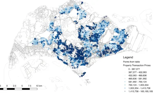
a geospatial layer of property prices was created. (Figure 3.4)

Figure 3.4: Mapped Property Transaction Records

Using this base layer of property prices, the average price of all transactions within a 400-meter straight-line radius of student’s recorded home location was derived. (Fig 3.5 below)

9 _{SLA, “API documentation: Address Search API”, http://www.onemap.sg/api/help/ . Accessed September 2016.}

Fig 3.5: Example of calculation of students’ neighborhood property prices High SES neighborhood (Bukit Timah):

Property sales’ average = SGD 12 million

Lower SES neighborhood (Boon Lay) : Property sales’ average = SGD 310,000

vi. Home - School Built Environment Characteristics

As discussed in the literature review, the built environment is likely to influence students’ walking behavior. Given previous analyses of the NSE data suggests that students tend to travel primarily between home and school neighborhoods (Wilhelm et. al 2016), measures of built environment characteristics around the twin anchors of home and school were thus added into the analysis.

To characterize the built environment, 16 different built environment measures were identified, drawing from commonly used categories and measures of the built environment in the health and transport literature. Land use, road and public transport network, and building-level data was compiled from available government agency data, as well as a synthetic building population dataset developed as part of the Singapore-MIT Alliance for Research and Technology (SMART)’s SimMobility project (Le et. al, 2016). (Appendix A provides data sources, calculation methods and descriptive statistics for each measure).

Density:

● Density of Built Area

Diversity: (Landuse mix & POIs)

● Number of Retail, Food and Beverage Outlets within buffer (from 2012 ACRA

dataset)

● Landuse Diversity Mix (FM synthetic building estimated use+ MP08 for parks &

openspace ) Access to Public Transit

● Count of Bus-stops within buffer

● Count of Mass Rapid Transit (MRT) stops within buffer

Design: Street network

● Length of expressways per unit area ● Length of major arterial roads per unit area ● Length of local roads per unit area

● Number of intersections within buffer area

● Percent of four-way intersections within buffer

● Density of four-way intersections

● Density of three-way intersections

● Density of porous walkable space – HDB parcels minus footprint and smaller parks (i.e. not Nature Reserves or Nature areas)

Design: urban form

● Average building footprint

● Average building heights

For the built environment analysis, suitable areal unit had to be defined. The Inland Revenue

Authority assigns a unique 6-digit postal code to every building in Singapore (Agarwal, et. al

2016). Thus, postal codes make for very fine-grained locational markers that have the

additional advantage of being easily relatable to existing administrative datasets. As this study

focuses on walking behavior, the areal unit of analysis is defined as a 500-meter street

network buffer around each postal code, which can be interpreted as the ‘walk-shed’ around each building. A student’s primary home and school environments are thus defined as the 500-meter walk-shed around the post-codes each location is closest to.

Rather than analyzed as discrete parameters with independent associations with walking behavior, the listed built environment measures were used to generate several ‘neighborhood types’ that collectively summarize and represent Singapore’s urban built environment. This approach of classifying the built environment into representative neighborhood types, which are then fed into further analysis about the potential impact of the built environment, has been used in several other physical activity and travel-related studies (McDonald et. al, 2012; Adams et. al 2013; Adams, et. al 2011;Todd et. al 2016).

There are several advantages of taking such an approach. As neighborhood environmental attributes are often correlated, it is challenging to examine the relationships of these attributes with physical activity through simple covariate adjustments without running into problems of multi-collinearity and potential over-adjustment. Evaluating clusters of built environment measures that co-occur, through neighborhood types, side-steps this problem (Adams et. al 2013). Furthermore, given that the combined effects of different built environment characteristics may prove more substantial than when taken individually, combining environmental measures into neighborhood types would better pick up built environment effects.

There are many different classification techniques. This study applied two established classification techniques--Latent Profile Analysis and K-Means—that have been used in other built environment studies, to the 16 built environment measures, generating two sets of neighborhood classifications for the entire island. These two sets of classification were assessed for interpretability, and also statistical explanatory power, when included in different runs of the study’s statistical models. Findings are discussed in the next section of this paper.

To reduce substantial overlap between buffer areas, as well as computational load, only postal codes that were at least 50 meters apart were used to generate neighborhood buffers. It is worth noting that even after dropping postal codes that were less than 50 meters apart, the generated buffers still overlapped, especially in very dense, built-up areas. All in all, built environment measures for 24,593 postal code buffers were calculated.

(Classification 1): Latent Profile Analysis

A latent profile analysis (LPA) seeks to recover hidden groups in the data based on the means of continuous observed variables. This technique has been used in studies across various disciplines, including ones on the built environment and physical activity, as a way to cluster or classify data (Adams et. al 2011; Todd et. al, 2016).

The analysis starts with an assumption that parameters of each hidden group follow a normal distribution. Initial estimates of the ‘within-class’ means and standard deviations of each group are made. Based on these estimates, a posterior probability of likelihood of belonging to one group is assigned to each observation. The posterior probabilities are then be used to update the estimate of ‘within-class parameters’, which is then used to update posterior probabilities, and so on until an equilibrium is reached. The ‘best’ number of latent classes is determined through comparison of posterior fit statistics, such as the Bayesian Information Criterion (BIC)—an information-theoretic method (Oberski , 2016).

For this analysis, I used R statistical package mclust (Fraley et. al, 2012). As each built environment variable differed widely in terms of units of measurement (e.g. counts, lengths in kilometers, percentages), variable values of each observation was normalized by subtracting

the mean and dividing by the standard deviation of each variable10, to avoid having the results being overly influenced by measures with larger scales.

The mclust function compares BIC values for up to nine components, and chooses a model with the best fit, according to its BIC value (Fraley and Raftery, 1998). For the built environment measures, a model with nine components—which can be interpreted as representing a ‘neighborhood type’—was identified as the most optimal model. For each of the 9 neighborhood types, the mean probability that each observations was correctly pegged to that type ranges 96% to over 99%, suggesting a good degree of classification accuracy. (see Appendix B.1 for details of model-fit)

The neighborhood type components were then examined for interpretability. For each neighborhood type, the means of all 16 built environment variables were compared against the mean and standard deviations of the full postal code buffers dataset, to identify patterns and dominant characteristics of each LPA-estimated type. (see Appendix B.2 for details of within-class parameter distributions). Figure 3.6 below summarizes the spatial distribution of these neighborhood types, and their key characteristics

Figure 3.6: Neighborhood Types generated by Latent Profile Analysis

1) TOD 1: Commercial Centers (n =744) - Very High Density, tall buildings with very large footprints - Many F&B, Retail outlets and good landuse mix - Well served by public transport (PT) - Well-connected road network 2) Fine-grained private housing estates (n=4,666) -Low density, low rise, small footprints -Few F&B, retail outlets and average use mix -Few PT options - Fine-grained road network

10 _{R-Manual, “Scaling and Centering of Matrix-like Objects”, https://stat.ethz.ch/R-manual/R-devel/library/base/html/scale.html}

3) Isolated areas (Industry & larger landed housing) (n=3,503) -Low density, low-rise -Poor use mix and very low F&B, retail -Poor access to PT -Poorly connected road network 4) Mixed: Private Condo areas, near parks (n=3,514) -Mid-high-rises -Average use mix and access to F&B and retail -Poor access to MRT -Non-grid like road network 5) Fine-grained commercial area (n=1,926) -Average height and density, with smaller footprints -Good F&B, retail outlet access and use mix -Poor access to MRT -Fine-grained road network 6) TOD2: HDB areas (n=1,418) -High-rise, medium-high density area -Many PT options -Large spreadout grid (i.e low junction count) -More porous space 7) Expressway areas (n=1,758) -Medium height, average density area with large building footprints and poorly served in terms of PT and F&B, retail outlets -Spread-out, poorly connected grid 8) HDB Areas (n=4,225) -Medium-height and high density, relatively poor use mix -Good bus-coverage -Spaced out, poorly connected road network 9) Industrial parks (n=2,839) -Mid-low rises, with large footprints -Low-mid use mix and provision of F&B and retail -Poor access to MRT -Grid-like road network

(Classification 2) K-Means: A similar classification process was carried out, but using k-means cluster analysis. K-k-means has been utilized in a wide variety of analysis, including the

classification of built environment measures in a limited number of studies (Szapocznik et. al,

2006; Jorge et.al 2012). The k-means algorithm partitions a large dataset into a predetermined ‘k’ number of clusters, while seeking to minimize the within-cluster sum of squares (Hartigan and Wong, 1979).

A scree plot, which shows the sum of squared distances of every observation to its cluster centroid for an increasing number of clusters, was used to determine the most appropriate number of clusters(Jorge et.al 2012). Based on the scree-plot, six clusters were identified as appropriate k, as a further increase of one cluster added very little reduction to the within-cluster sum of squares. (see Appendix B.3 for plot)

The ‘stats’ package in R was used to classify the 24,593 postal code buffers into 6

neighborhood types, using a scaled set of variables for similar reasons mentioned for the LPA analysis.

As before, the six neighborhood types were examined for interpretability, and the means of the 16 building environment variables for each type were compared against the mean and standard deviations of the full BE dataset (see Appendix B.4 for details of within-class parameter distributions). Figure 3.7 below summarizes the spatial distribution of these neighborhood types, and their key characteristics

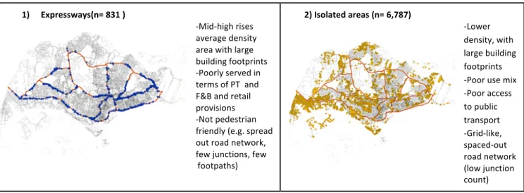
Figure 3.7: Neighborhood Types generated by K-means clustering

1) Expressways(n= 831 ) -Mid-high rises average density area with large building footprints -Poorly served in terms of PT and F&B and retail provisions -Not pedestrian friendly (e.g. spread out road network, few junctions, few footpaths) 2) Isolated areas (n= 6,787) -Lower density, with large building footprints -Poor use mix -Poor access to public transport -Grid-like, spaced-out road network (low junction count)

3) Fine-grained estates (n=6,744 ) -Lower density, low-rise area, with small buildings -Pedestrian friendly, fine-grained local road network and many junctions 4) TOD (n=3,356 ) -High-rise, high density areas -Good access to public transport -Flanking arterial roads 5) High Density Commercial Areas (n= 517) -Very high-rise, high density, large footprints - Good use mix, high F&B and retail provision -Many PT options -Fine grained local road network( many junctions) 6) HDB areas (n= 6,358 ) - High-rise, high density areas -Comparatively poorer access to public transport -Fewer arterial roads and less ‘grid-like’

Checking for Concurrence

To check how much agreement there is between the two classification methods, an Adjusted Rand Index (ARI) was calculated, using the R ‘mclust’ package. The Rand index compares the two partition, and calculates the amount of overlap between two partitions (in this case, one set of neighborhood types derived using k-means, and the other using LPA). If the dataset is split into pairs of observations, each pair can be assessed as:

i Belonging to same class in Partition 1 and in the same class in Partition 2; ii Belonging to different classes in Partition 1 and in different classes in Partition 2; iii Belonging to different classes in Partition 1 and in the same class in Partition 2; iv Belonging to the same class in Partition 1 and in different classes in Partition 2. Pairs that fall under i and ii can be considered as ‘agreeing’, while those under iii and iv are ‘disagreeing’. The original Rand index thus estimates the percentage of possible pairs that ‘agree’. The ARI corrects for chance, where the two partitions are picked at random is given a zero expected value, and where total agreement between the two partitions are given a value of 1. The ARI can thus be interpreted as the (normalized) difference of the Rand Index and its

expected value under the null hypothesis of a random partition (Hubert and Arabie, 1985). A high ARI value approaching 1 suggests high degrees of agreement, while low values approaching 0 suggest low degrees of agreement between the two classifications.

Besides being a well-established metric, the ARI was picked for study because it is suitable for measuring agreement between two partitions in clustering analysis with different numbers of clusters, as is the case in this study. The ARI is also suitable for unbalanced datasets where one cluster has a very large percentage of all observations, since the index analyzes each pair of elements and measures the relationship between elements of the same class more so than the relationship between each observation and its classification (Santos and Embrechts, 2009).

Comparing the k-means and LPA clustering yields an ARI of 0.334, a fairly low score that suggests a substantial degree of non-agreement between the two classification approaches. Identifying the reason behind the low degree of concurrence would require more analysis, but what this ARI score suggests is that these two classifications cannot be seen as interchangeable. However, as it is not intuitively clear upfront which set of neighborhood types would work better in explaining variations in walking behavior, both sets were used in subsequent analyses.

c. Data filtering procedures

While the full, unfiltered dataset included data records of close to 40,000 students and over 136,000 days of data, some of the exhibited travel patterns were not consistent with expected movements or location patterns of a typical student. The data was thus filtered to sieve out potential errors in data logging or sensor use, as described below:

i. Home and School Locations

Based on SUTD’s home/ school location estimates, some students had either no ‘home’ location identified, and or no corresponding ‘school’ location identified. Some students had multiple home and school locations identified that were beyond 200 to 300 meters apart, which cannot be chalked up to simple sensor accuracy errors. Observations from approximately 20,000 students who exhibited these inconsistencies were dropped from the full dataset, leaving data from about 22,000 students.

ii. Morning Mode Categorization

Morning transport modes were identified for approximately 10,200 students, with about 16,000 days of logged data. Approximately 11,000 students who were not tagged with a morning mode were not included in the analysis.

iii. School Characteristics

The majority of schools in Singapore are single-session, starting in the morning and ending in the afternoon. In 2015 however, there were still 32 Primary schools that had yet to switch to single session. This meant some students in these ‘non-single session’ schools started lessons in the afternoon, and thus did not have a similar morning commute as the majority of students.

Given that all Singaporean primary schools are slated to be single-session schools in the near

future (Parliament of Singapore, 2012) and that any future policy on commuting-based

initiatives would be targeted at single-session schools, the analysis was focused on the commutes and walking behavior of single-session students. For this reason, students from the 15 non-single session schools included in the NSE initiative were not included in the final dataset.

While most schools in Singapore are single-level schools, there are a few that include both secondary and primary school levels. It was thus not possible to identify which students from these schools are younger primary school students or older secondary school students. For the analysis that requires differentiation by age groups, students from these non single-level schools were not included, leaving a sample of about 10,000 students.

iv. Home-school distance

Some students that have been coded as having walked to school registered an unrealistically long home to school distance of up to 11km. A manual spot-check of a few examples revealed unrealistically short commute times that would be physically impossible for a human travelling on foot to achieve. A three km home-school distance threshold was thus established to sieve out 345 ‘unrealistic walkers’, as students are unlikely to choose to walk extremely long distances to school as their regular commute, given Singapore’s hot and humid weather.

v. Number of steps

Some students registered very low number of steps, which fell way below what could be considered a reasonable ‘basal’ level of activity. For adults, a basal amount of walking has been estimated about 2,500 steps per day (Tudor-Locke et. al, 2011). There does not seem to be a similar benchmark for children and teens, but a recent study estimated that the most

sedentary 19-year old females at the 5th _{percentile of walking activity walked up to 1,100 steps}

while similarly sedentary 6 year-old females at the 5th percentile of ‘activeness’ walked up to

5,600 steps (Barreira et.al, 2015).

Extremely low step counts may partially be explained by the sensor’s inability to pick up short spurts of walking activity, but may also be explained by inappropriate use of the sensor. For instance, a student may leave his/her sensor unattended for long periods of time. To sieve out the latter case, as a last step of filtering, a low floor of a minimum number of steps was applied to the dataset. Students who logged fewer than 200 steps throughout the day, or logged fewer than 100 steps within 800-meter radius of their registered school or home location, or who registered zero steps before 8am were dropped from the analysis. (n = 1,058) This final step of filtering brings the total study population to 7,688 students.

vi. Availability of Neighborhood Property Price Transactions data

Another 15 students were dropped from the dataset as there were no property transaction data available for the immediate neighborhood in which they were living.

The final dataset used in this analysis thus consisted of 7,673 students. These students represent participants who:

● Logged at least 1 day of data that indicated their presence at a consistent, defined home and school location,

● Can be reasonably identified as Primary, Secondary or JC student who commute to school in the morning

● Have a morning travel mode identified ● Logged a minimum number of steps

● Has an approximate household SES measure associated with them

A sensitivity analysis was conducted, where data that was not filtered by number of steps was used for the analysis. Details of the sensitivity analysis are included in section IV.

IV. Analysis Results

a. Descriptive Statistics of the NSE data

The following paragraphs present summary statistics of the key variables of this study, compared against existing data where possible, to help establish greater confidence in whether the NSE data is accurate and reflective of previously observed trends.

i. Mode Split

Of the 7,673 students included in this analysis, 3,411 (44%) were primary school students, 4,028(53%) secondary school students, and 224 (3%) junior college students.

The mode classification split of this study’s sample was compared to the estimated mode split estimated from Singapore’s 2015 General Household Survey (GHS), to gauge whether the NSE data was representative of Singaporean students’ commuting behavior. Across both studies, the older students tended to be more likely to take public transport, while the younger primary school students tended to walk more or be driven to school (Fig 4.1). However, the NSE dataset includes a larger proportion of students classified as ‘walking’ to school than the GHS 2015. Possible explanations for the difference are that the NSE dataset oversampled walkers or that the mode classification algorithm may have classified more commutes as ‘walking’ than accurate.

Fig 4.1: Mode Choice Split of students (by Grade Level) – NSE compared to GHS 2015

17% 67% 16% 7% 88% 4% Car Public Transport Walking JC NSE (n = 2,44) GHS (n = 58,500) 23% 12% 65% 32% 20% 43% Car Public Transport Walking Primary NSE (n = 3,411) GHS (n = 262,100) 19% 40% 42% 12% 70% 16% Car Public Transport Walking Secondary NSE (n = 4,038) GHS (n = 205,600)

ii. Number of Steps

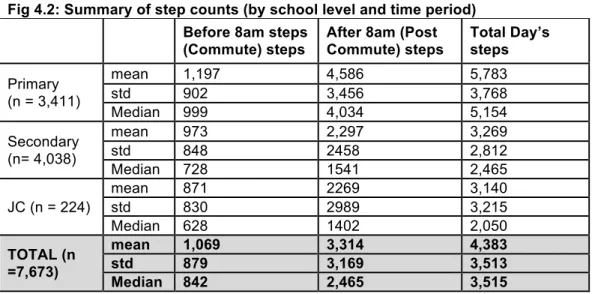
Consistent with findings from previous studies of children’s walking patterns described in the literature review, the older students in this dataset tended to take fewer steps than their younger counterparts. Fig 4.2 and Fig 4.3 below summarizes the steps taken at three time periods: 4am to 8am; 8am till midnight; 24 hours of the day.

On average, primary school students took 20% of their total daily steps before 8am, while secondary and JC students logged about 30% of their daily steps before 8am. Commutes thus did consist of a sizeable chunk of students’ daily walking activity.

Fig 4.2: Summary of step counts (by school level and time period) Before 8am steps

(Commute) steps

After 8am (Post Commute) steps Total Day’s steps Primary (n = 3,411) mean 1,197 4,586 5,783 std 902 3,456 3,768 Median 999 4,034 5,154 Secondary (n= 4,038) mean 973 2,297 3,269 std 848 2458 2,812 Median 728 1541 2,465 JC (n = 224) mean 871 2269 3,140 std 830 2989 3,215 Median 628 1402 2,050 TOTAL (n =7,673) mean 1,069 3,314 4,383 std 879 3,169 3,513 Median 842 2,465 3,515

Fig 4.3: Frequency Distributions of Students’ Steps (by Grade Level and Time Period)

Before 8am (commute) steps After 8am steps Total Day’s Step