an author's https://oatao.univ-toulouse.fr/27091
https://doi.org/10.1109/MAES.2017.150260
Vilà-Valls, Jordi and Closas, Pau and Navarro, Monica and Fernández-Prades, Carles Are PLLs dead? A tutorial on kalman filter-based techniques for digital carrier synchronization. (2017) IEEE Aerospace and Electronic Systems Magazine, 32 (7). 28-45. ISSN 0885-8985
Carrier synchronization is a fundamental stage in the receiver side of any communication or positioning system. Traditional carrier phase tracking techniques are based on well-known phase-locked loop (PLL) closed-loop architectures, which are still the methods of choice in modern receivers. Those tech-niques are well understood, easy to tune, and perform well under benign propagation conditions, but their applicabil-ity is seriously compromised in harsh propagation environ-ments, where the signal may be affected by high dynamics, shadowing, strong fadings, multipath effects, or ionospheric scintillation. From an optimal filtering standpoint, the Kal-man filter (KF) is clearly a powerful alternative, but the syn-chronization community seems still reluctant to exploit all the potential it has to offer. The purpose of this article is twofold:
i) to review the basics and state of the art on both PLL and
KF-based tracking techniques and ii) to present and justify the reasoning behind the systematic use of KF-based tracking approaches instead of the well-established PLL-based archi-tectures from both theoretical and practical points of view. To support the discussion, two specific scenarios of interest to the aerospace community are numerically evaluated: robust car-rier tracking of global navigation satellite systems' signals and synchronization in a deep space communications system.
INTRODUCTION
The main goal of this article is to provide a tutorial-style discus-sion on why traditional synchronization loop architectures, inherited from the analog era, may be abandoned in modern digital receivers and to move forward toward the design and actual use of more flex-ible, robust and powerful Kalman filter (KF)-based synchronization schemes. Carrier synchronization is a key process in most electronic devices involved in aerospace systems, and it is typically carried out following a two-stage approach: acquisition and tracking. The first stage detects the presence of the desired signal and provides a coarse estimate of its synchronization parameters, and the second one re-fines those estimates, filtering out noise and tracking any possible time variation [1]. In the present work, we are concerned with the analysis of the carrier phase (CP) tracking problem. Hence, acquisi-tion and time delay synchronizaacquisi-tion are not discussed.
Digital CP tracking techniques implemented in conventional re-ceivers rely on well-known phase-locked loop (PLL) architectures [2], [3], [4] that set an output signal's phase relative to an input reference signal's phase. Those circuits are widely used in positioning systems, communications, computers, control, and measurement applications for frequency synthesis, clock and data recovery, clock distribution, and other more specialized functions. The signals of interest may be any periodic waveform but are typically sinusoids or digital clocks.
Digital PLLs can be implemented in hardware (usually with mixed signal or all-digital integrated circuits in complementary metal oxide semiconductor technology [5], [6], [7] and targeting frequencies on the order of gigahertz and above [8]), but the rapid evolution of program-mable devices, such as field-programprogram-mable gate arrays, digital signal processors, microcontrollers, and general-purpose processors, enables software-defined implementations targeting frequencies up to hundreds of megahertz, in which the designer trades electronic components for computation resources [9], [10]. This approach provides advantages, such as easy customization of the feedback loop and a drastic reduction in the development cost, when compared with the hardware counter-part. However, the underlying design principles remain the same re-gardless of the technology of choice for the implementation.
The performance obtained with those techniques is generally good enough in benign propagation conditions, but they have been shown to deliver poor estimates or even fail under harsh propa-Authors' current addresses: J. Vilà-Valls, M. Navarro, C.
Fernández-Prades, CTTC, Statistical Inference for Communi-cations and Positioning, Centre Tecnològic de Telecomunica-cions de Catalunya, Carl Friedrich Gauss, 7 Castelldefels, Bar-celona 08860 Spain, E-mail: ({jordi.vila,monica.navarro,carles. [email protected]); P. Closas, Department of Electrical and Computer Engineering, Northeastern University, Boston, MA 02115, USA. E-mail: [email protected]
This work was supported by the Spanish Ministry of Economy and Competitiveness through project TEC2015-69868-C2-2-R (ADVENTURE) and by the Government of Catalonia under grant 2014–SGR–1567.
Are PLLs Dead? A Tutorial on Kalman Filter-Based
Techniques for Digital Carrier Synchronization
Jordi Vilà-Valls, Centre Tecnològic de Telecomunicacions de Catalunya (CTTC/CERCA),
Barcelona, Spain
Pau Closas, Northeastern University, Boston, MA, USA
Monica Navarro, Carles Fernández-Prades, Centre Tecnològic de Telecomunicacions de
gation environments, where the signal may be affected by high dynamics, shadowing, strong fadings, multipath effects, or iono-spheric scintillation [11], [12]. On the basis of conventional PLL architectures, some improvements have been proposed in the lit-erature [13], [14], [15], but their performance have been overcome by KF-based techniques [11], [12], [16], [17], [18]. The main draw-back of KFs is the need of an exact knowledge of the system model noise statistics' for an optimal behavior, thus being constrained by the accuracy of the dynamic model and the a priori fixed system parameters. In practice, those quantities may need to be somehow adjusted to provide a robust solution [19], a problem that has been solved by the so-called adaptive KFs (AKFs) [19]–[24].
Our previous experience on the use of KF synchronization schemes for both communications [25], [26] and positioning systems [19], [27], [28], [29], the lack of a unified analysis in the literature, and a clear answer to the PLL versus KF dilemma ignited this work. From different analysis carried out in the literature for specific scenarios, it seems clear that KF schemes should, in general, be preferred in front of PLL-based solutions, but the synchronization and aerospace communities seem still reluctant to go further on theoretical analysis of such techniques and to cross the gap between theory and implementation. Moreover, the ad-vent of software-defined radio receivers in real-life applications [30], [31] has confirmed the practical feasibility of this approach. The main goal of this tutorial-style article is to provide a comprehensive overview and unified framework. Therefore, this work is for the practitioner or engineer who needs to solve real hands-on problems and the academic or researcher willing to push forward on new advanced synchronization techniques.
The notation used in this article is as follows: lowercase italics for scalar variables, either deterministic or stochastic, both real or complex; uppercase italics for constants; lowercase bold for vec-tor variables, columnwise defined; uppercase bold for matrix vari-ables; (·), (·)*, and (·)H stand for the transpose, conjugate, and
conjugate transpose (hermitic) operators, respectively; is an esti-mate of the true parameter value x at time k, given its value in time
k – 1;x ∼ ( , )2
x x
μ σ
is a random variable x Gaussian-distributed with mean μx and variance σx2; and ℜ(x) and I(x) stand for the real
and imaginary parts of x, respectively. More notation will be de-fined throughout the article, as needed.
PLL-BASED ARCHITECTURES
CP synchronization techniques implemented during recent decades in mass-market and industrial-grade positioning, communications, and tracking systems receivers rely on well-established PLL-based architectures [4], [32], [33]. First analyzed by Appleton in 1922 [34], early applications of PLLs were the control of receivers' local oscillators, especially in FM demodulators and automatic volume control circuits. In the early 1950s, they played an important role in the development of color television [35], and the availability of PLL integrated circuits in the mid-1960s facilitated their rapid introduction into a wide range of consumer products, becoming a key component of electronic devices for the next three decades [36], [37], [38]. Nowadays, digital PLLs are widely used in mod-ern communication systems [39] and are still the method of choice in many applications, such as global navigation satellite systems (GNSS) [3] and space communications [40], mainly because of manufacturer's inertia on legacy solutions and well-proven tech-nologies. Hereafter, the main PLL-based architectures and design rules are summarized.
BASICS
In general, a PLL is built up with three main blocks: the discrimina-tor or phase detecdiscrimina-tor, the loop filter, and a numerically controlled oscillator (NCO), which is nothing but an integrator. The main idea is to obtain first an error signal (i.e., discriminator's output), which is proportional to the CP error; then, this error goes through the loop
Figure 1.
filter, in charge of filtering out noise and driving the error to zero; and finally, the NCO is used to generate the local replica (i.e., a complex exponential using the predicted or tracked CP). The basic PLL architecture is sketched in Fig. 1.
The role of the phase discriminator is to produce an output that is proportional to the phase estimation error. In the presence of data modulating the phase of the input signal (and thus producing phase jumps), noncoherent discriminators (usually known as Costas-type discriminators) should be adopted. The two quadrant arctangent discriminator atan (I(yk)/ℜ(yk)) is usually the preferred noncoherent
choice [3], although other discriminators may result from differ-ent optimization criteria and signal-to-noise ratio (SNℜ) regimes [41], [42]. Otherwise, if phase jumps produced by data have been removed (either because they belong to a training sequence known at the receiver or because they have been estimated) or pilot (data-less) signals are available, coherent discriminators may be used [39]. In the absence of data, the optimal maximum likelihood (ML) estimator is the four-quadrant arctangent discriminator atan2 (I(yk)/ℜ(yk)). In addition to the phase discriminators, one may be
interested in directly tracking the input signal frequency by using a frequency-locked loop (FLL). ℜefer to [43] for detailed analysis and an updated overview on carrier tracking techniques.
The order of the PLL refers to the overall closed loop (used throughout the article to unify the notation) and not only to the filter loop, which may lead to confusion because the latter is al-ways one order lower than the entire loop due to the NCO. The order of the PLL basically determines the input signal dynamics that the filter is able to track. In other words, a second-order PLL is able to track a constant frequency mismatch, whereas a third-order PLLs properly tracks frequency drifts. The loop coefficients are usually optimized to minimize the mean-squared error (MSE) [3], but other approaches may be adopted as well [44].
The dynamics of a PLL are heavily dependent on the type and response of the loop filters. A PLL with nth order filter is of (n + 1)th order. In the general case, a PLL of order n has a closed-loop transfer function that can be expressed as [45]
( ) PI( ) ( ), H s =H s L s (1) where HPI(s) = K1 + 2 3 2 ... K K
s + s + is the transfer function of the
proportional plus integrator part, Ki is the gain of the loop of order
i, and L(s) is the transfer function of the loop filter.
ANALOG VERSUS DIGITAL
To start from scratch and see how digital PLLs are derived from their analog design, some results on analog PLLs are given togeth-er with their digital counttogeth-erpart.
Analog PLLs
The Laplace transform of the continuous time domain transfer functions for the second- and third-order PLL loop filters are, re-spectively, 2 2 2 3 2( ) n n ; 3( ) n 2 n n, a s c s b s L s L s s s ω +ω ω + ω +ω = = (2)
where a, b, and c are the loop filter coefficients, and ωn (radian
per second) is the so-called natural frequency of the loop filter. The PLL loop is closed with a voltage-controlled oscillator (VCO), with transfer function V(s) = 1/s (unity VCO gain). The closed-loop transfer functions for these second- and third-order PLLs are
2 2( ) 2 n n 2, n n a s H s s a s ω ω ω ω + = + + (3) 2 2 3 3( ) 3 n 2 n 2 n 3. n n n c s b s H s s c s b s ω ω ω ω ω ω + + = + + + (4)
The single-sided loop noise bandwidth Bn in hertz (defined as the
bandwidth of a perfect rectangular filter that produces the same integrated noise power as that of the actual filter) is obtained from the frequency response (setting s = j2π f) of the closed-loop system as
(
)
2, 0 2 ,
n i i
B =
∞H j πf df (5)where i is the loop order. This bandwidth can be used to compute the receiver's noise floor (kTBn) and its sensitivity (the minimum input
signal power required to produce a specified SNℜ at the receiver's output). Equation (5) can be analytically computed from the loop parameters and the natural frequency [3]. Again, considering the second- and third-order loops, the noise bandwidth can be written as
(
)
2 2 2 ,2 2 ,3 1 ; . 4 4( 1) n n n n bc b c a B B a ω bc ω + − + = = − (6)Therefore, the design of the analog PLL is completely specified by the desired noise bandwidth and the filter parameters, which are usually designed to minimize the estimation's MSE. Typical values are [3] a = 2, b = 1.1, and c = 2.4, which is the setup used in the literature to compute the PLL parameters from a specified noise bandwidth.
Digital PLLs
Digital PLLs are usually derived from their analog counterpart. Using s = (1 − z−1)/T
s, with Ts the sampling period, one can obtain
the PLL loop transfer function and the overall closed-loop transfer function. In this case, the VCO is replaced by a NCO with transfer function 1 1 ( ) . 1 z N z z − − = − (7)
Considering the following loop filter transfer functions [15]
2 2( ) 1 1 1, L z z α α − = + − (8)
(
)
2 3 3( ) 1 1 1 1 2, 1 L z z z α α α − − = + + − − (9)the discrete-time closed-loop transfer function for the second- and third- order PLLs are
(
1 2)
1 2 2 1 2 ( ) , ( 1) ( 1) z H z z z z α α α α α + − = − + − + (10) 2 3 3 2 2 1 2 3 ( ) , ( 1) ( 1) ( 1) H z z z z z z α α α α = − + − + − + (11)where the loop filter coefficients can be directly computed from the analog loop filter parameters, the desired noise bandwidth and the sampling period as
C second order: α 1 = aωnTs and α2ωn s2 2T. C third order: α 1 = cωnTs, α2 = 2 2 n s b Tω and α3 = 3 3 n sT ω .
For the digital PLL, the equivalent noise bandwidth can be directly computed from H(z) (results given in hertz) [15], leading to
(
)
2 1 2 1 2 ,2 1 1 2 2 2 , 2 4 2 n s B T α α α α α α α + + = − − (12) 3,1 ,3 3,2 3,3 , 2 n s B T γ γ γ = (13) with γ3,1 = 2 1 2 4α α − 4α1α3 + 2 2 2 2 1 2 1 3 4α +2α α +4α α + 4α2α3 + 3α1α2α3 + 2 2 3 1 3 α +α α , γ3,2 = α1α2 − α3 + α1α3 and γ3,3 = 8 − 4α1 − 2α2 − α3. These results verify that digital PLL parameters computed from the analog coefficients are equivalent to the parameters di-rectly derived in the discrete-time domain, because the resulting equivalent noise bandwidths coincide.STANDARD AND ADVANCED PLLS
A key step for the practitioner may be how to interpret (8) or (9) and the way to turn them into a useful architecture. The block dia-gram of a third-order PLL loop filter is sketched in Fig. 2. The standard PLL-based architectures are somehow limited because of the noise reduction versus dynamic range trade-off, which may lead the filters to lose lock.
This trade-off is mainly driven by the bandwidth and order of the loop. A small bandwidth is needed to filter out as much noise as possible to be able to operate at low SNℜ, whereas a large one is required for coping with fast variations of the parameters of interest. Moreover, the loop's order also plays an important role in such scenarios. For instance, the second-order PLL is uncon-ditionally stable at all noise bandwidths, but it is not suitable to deal with complex dynamics. The third-order PLL, while being more flexible in front of high dynamics, only remains stable for bandwidths below 18 Hz [3]. Another issue is the PLL constant bandwidth, a priori fixed by the designer. A time-varying
band-width would seem to be more suitable in practice. These two key points have led to propose a plethora of advanced PLL-based techniques.
One possible solution to provide robustness and extra flex-ibility to the stand-alone PLLs is to consider cooperative loops
architectures, where several loops interact to counteract its
in-dividual limitations. The most basic solution is the so-called
switching architecture, where a PLL is used under nominal
op-eration but the system switches to a FLL in harsh conditions to not lose lock [46]. The FLL is, in general, more robust than the PLL because the variability of the incoming signal frequency is orders of magnitude lower than the phase variability. How-ever, the solution usually adopted to overcome the problems of standard architectures in dynamic or harsh conditions is the use of a hybrid approach in which the FLL permanently assists the PLL (F-PLL) [13], [47], which is capable to maintain lock in situations in which the PLL diverges. The second concern that typically arises from standard architectures is the constant band-width operation, which may limit its applicability to rather con-stant propagation conditions. A possible solution is to directly use the input working conditions to automatically adjust the loop bandwidth, what is usually known as adaptive bandwidth PLL (A-PLL) [48]. Several contributions appeared in the literature using the same concept [15], [49], [50].
The following section presents a systematic, unified approach to design digital phase tracking filters that is based on the techni-cally sound Bayesian filtering theory.
STANDARD KF-BASED CARRIER TRACKING
OPTIMAL FILTERING BACKGROUND AND KF GENERAL
FORMULATION
The optimal filtering problem involves the recursive (i.e., online) estimation of time-varying unknown states of a system by using the incoming flow of information (observations) from the system, along some prior statistical knowledge about the variations of such states. The general dynamic state-space model (assuming additive noises) can be expressed as
( )
1 1 , k = k− k− + k x f x ν (14)( )
, k = k k + k y h x n (15)Figure 2.
where xk∈Rnx and yk Ry n
∈ are the hidden states of the system and measurements at time k, fk–1(·) and hk(·) are known, possibly
nonlin-ear functions; νk and nk are referred to as process and measurement
noises (assumed mutually independent stochastic processes). The optimal Bayesian filtering solution [51] is given by the marginal distribution p(xk|y1:k),1 which gathers all the information about the system contained in the available observations. This distribution can be recursively computed in two steps: i) prediction, the predic-tive distribution p(xk|y1:k−1) is computed using prior information,
p(xk | xk−1), and the previous distribution, and ii) update, the new
measurements yk and the predictive distribution (see Algorithm 1
in [53]) are used to obtain the new filtering distribution p(xk|y1:k). The standard KF [51], sketched in Algorithm 1,2 provides the closed-form solution to the optimal Bayesian filtering problem in linear and Gaussian systems, assumptions that not always hold. A plethora of alternatives have been proposed in recent decades to solve the nonlinear estimation problem. Among them are the ex-tended KF (EKF) [51], the family of sigma-point KFs [54] within the Gaussian framework and the family of sequential Monte Carlo methods [55] for arbitrary noise distributions. The carrier synchro-nization problem is just a particular application case of this general filtering solution.
The probabilistic assumptions made by the KF are vk ∼
(0,Qk) and nk ∼ (0,Rk), with Qk and Rk being the process and
measurement covariance matrices, respectively. For linear dynam-ic systems, the KF always provides the linear MMSE solution, but if the process or measurement noises are not Gaussian distributed, the KF is no longer optimal. The filter uses a Gaussian approxima-tion and only propagates the mean and covariance of the predictive and posterior distributions, so intuitively the further from
Gaussi-anity, the further from optimality.
The filtering equation in Step 7 of Algorithm 1 reveals how the KF estimation works
(
)
| 1 1| 1 | 1
state prediction measurement update
ˆk k= k−ˆk− −k + k k−ˆk k− .
x F x K y y
(16)
Algorithm 1 General KF formulation Require: x Pˆ ,0 x,0|0, ,F H y Qk k, ,k k andRk∀k
1: Set k ⇐ 1
Time update (prediction)
2: Estimate the predicted state: xˆk k| 1− =F xk−1ˆk− −1| 1k .
3: Estimate the predicted error covariance:
, | 1 1 , 1| 1 1 .
x k k− = k− x k− −k k− + k
P F P F Q
Measurement update (estimation)
4: Estimate the predicted measurement: yˆk k| 1− =H xk k kˆ | 1−.
5: Estimate the innovation covariance matrix:
, | 1 , | 1 .
y k k− = k x k k− k + k
P H P H R
1 The characterization of the posterior distribution allows us to
compute the minimum mean-squared error (MMSE), the maxi-mum a posteriori (MAP), or the median of the posterior (mini-max) estimators, addressing optimality in many senses [52].
2 The standard filtering notation is used, where the subscript k|k−1
stands for prediction at time k using measurements up to time
k−1 and k|k refers to the estimation at time k, including the
com-plete measurements set y1:k.
6: Estimate the Kalman gain: 1
, | 1 , | 1
k= x k k− k y k k− −
K P H P .
7: Estimate the updated state: xˆk k| =xˆk k| 1− +K yk
(
k−yˆk k| 1−)
.8: Estimate the corresponding error covariance:
, | , | 1 , | 1.
x k k = x k k− − k k x k k−
P P K H P
9: Set k ⇐ k + 1 and go to step 2.
The first term takes into account the state evolution model to pre-dict the state at the following time step, while the second one cor-rects this prediction by incorporating the information provided by the new measurement yk. The term yk − yˆk k −| 1 is called innovation,
which can be seen as an error signal and a key part of the KF the-ory. If the filter is optimal, the innovations' sequence is a white Gaussian process, which is a useful theoretical result to build con-sistency tests [56], [57].
The innovations are weighted by the time-varying Kalman gain
Kk, which is computed by using the uncertainty of the state-space
model (i.e., noise statistics) and the covariance of the estimation error (i.e., how good the state estimation is)
(
)
1 , | 1 , | 1 . k x k k k k x k k k k − − − = + K P H H P H R (17)Observing the terms involved in the gain computation, and with a slight abuse of language, the following effects can be de-duced: i) increasing the measurement noise Rk, or equivalently
the uncertainty on the observation, reduces Kk; thus, the filter is
less confident on the information provided by the observations;
ii) on the other side, increasing the system model uncertainty, Qk,
increases Px,k|k–1 and, in turn, Kk. In this situation, more weight
is given to the observations and less to the state prediction. If the system is observable (i.e., the system states can be altered by changing the system input) and controllable (i.e., the value of the initial state can be determined from the system output), the filter tends to an asymptotic regime [58], that is, both Kk
and the estimation error covariance matrix tend to steady-state fixed values,
, |
limk→∞Kk →K∞ ; limk→∞Px k k→P∞. (18) These values only depend on the transition matrices and both process and measurement noise statistics and thus can be com-puted off-line. The steady-state error covariance is obtained by solving a discrete algebraic ℜiccati equation, and the steady-state gain is straightforwardly derived from this covariance ma-trix (Fig. 3). The use of such constant gain may be really useful in applications, where computational complexity is a very criti-cal point, because a steady-state convergence ensures that the gain in Equation (16) does not need to be recomputed at each time instant (that is, Kk = K∞). In this case, note that during the transient time, the filter is no longer optimal, and the ℜicatti equation may not converge [59].
The KF formulation is only valid for linear systems, but in many real-life applications, the measurement function, the state evolution, or both may be nonlinear. A classical solution is to use the so-called EKF, which uses a linearization of such nonlinear
functions and directly applies the KF equations. The key point is to use linearized transition matrices (Jacobian matrices), such as3
( )
( )
1| 1 | 1 ˆ ˆ 1 1 1 ; , k k k k k k k k k k − − − − = ∇ − − = ∇ x x F f x H h xand plug them into Steps 3, 5, and 7 of Algorithm 1. Notice that in Steps 2 and 4, we can use nonlinear functions. It is beyond the scope of this article to provide a detailed discussion on KF theory; for further details on the topic, refer to [51], [60].
CARRIER TRACKING STATE-SPACE FORMULATION
It is usually assumed that the phase variations of the signal of inter-est are due either to the relative movement between the transmitter and the receiver or to synchronization mismatches, and on top of it, there is a random behavior due to the noises affecting the system. The state-space formulation of this problem is defined via both process and measurement equations, as shown hereafter.
Carrier Tracking Process Equation
1 1 ,
k = k− k− + k
x F x ν (19)
where the additive noise includes any possible modeling mismatch. The state to be tracked includes the CP and the Doppler frequency terms (i.e., using a Taylor series expansion of the CP and truncat-ing at the order of interest), and the so-called transition matrix Fk–1
defines the phase evolution due to receiver dynamics. For instance, assuming that tracking phase θk (radian), Doppler shift fk (hertz),
and Doppler frequency rate fk (hertz per second) are enough for a
given application (i.e., assuming a third-order Taylor approxima-tion of the phase), the phase is
2 2
0 2 12 ,
k f kTk s f k Tk s
θ = +θ π +
(20)
where k refers to the discrete-time instants and Ts is the sampling
period. In this scenario, the state to be tracked is xkθk f fk k
, and the transition matrix is given by
3 The vector differential operator is defined as ∇ = [∂/∂x
1,...,∂/∂xn]. 2 1 1 / 2 0 1 , 0 0 1 s s k s T T T − = F (21)
where the phase is expressed in cycles (radian/2π). It is straight-forward to extend this state formulation to higher-order frequency terms if needed.
Carrier Tracking Observation Equation
Two cases may be considered: i) the measurements are noisy CP
observables (linear equivalent model); and ii) the observations are
directly the received signal baseband complex samples.
C Linear observation equation: the inputs to the carrier
track-ing block are linearly related to carrier observables,
lin lin
, ,,
k = k k+ θk →yk =θk+nθk
y H x n (22)
with Hk the measurement transition matrix and nk the
mea-surement noise, including thermal and phase noise contribu-tions, as well as other propagation disturbances.
C Nonlinear observation equation: the inputs to the carrier
tracking block are the complex baseband signal samples, which are nonlinearly related to the carrier observables,
( )
jk ,k = k k + k→yk =γkeθ +nk
y h x n (23)
with hk(·) the nonlinear measurement function, and γk refers
to the time-varying envelope of the received signal, which may be affected by different propagation disturbances such as fading, multipath, or scintillation.
Early approaches to this problem, such as the α-β and the α-β-γ filters [61], do not require a detailed system model, trading com-putational load by a degradation in performance with respect to the KF [62] due to their static, heuristically chosen gains.
KF-BASED CARRIER SYNCHRONIZATION ARCHITECTURES
In this section, different architectures to implement the KF-based carrier tracking solution are provided, coupling the general formu-lation given in Section III.A with the specific state-space model of Section III.B [16], [25].Linear Observation Architectures
The inputs to the tracking block are directly phase observables and thus use the state-space model defined by (19) and (22). Note that this architecture is called standard linear KF throughout the article, but in the literature, it is also referred to as direct-state KF [16]. The closed-loop block diagram is sketched in Fig. 3. An alternative linear architecture named error-state KF or rate-only feedback loop, typically used in GNSS [63], [64], is presented and
Figure 3.
Linear KF-based carrier tracking architecture with noisy carrier obser-vations.
analyzed in [16], with respect to the standard (direct-state) KF. The idea consists of using a state-space model, where the filter does not track directly the CP but the phase error. As it does not provide any advantage over the standard KF, the latter is preferred for practical applications.
Nonlinear Observation Architectures
The previous linear architecture is of limited applicability in real-life implementations. At least, some extra information should be added to explain how the phase observables are obtained. The standard solution is to use a discriminator, as done in traditional PLL architectures (Case 1), but the complex samples of the re-ceived baseband signal can be directly treated using a nonlinear filter (Case 2).
C Case 1, discriminator-based traditional approach:
Using a discriminator allows the use of a traditional KF, avoids the derivation of suboptimal solutions, and is con-sidered the reference KF-based architecture [43]. The main differences with the linear standard KF are i) the carrier gen-erator block, which uses the nonlinear observation equation
hk(·) and ii) the discriminator as phase detector. The block
diagram is shown in Fig. 4 (top).
C Case 2, EKF solution:
Using a discriminator might break the Gaussianity assump-tion within the KF, making the filter not optimal anymore, which may lead to poor filter performances or even diver-gence. Moreover, the discriminators may need to operate un-der saturation in low SNℜ scenarios. A solution is to directly deal with the nonlinear Gaussian observation model [25], [26]. The simplest solution is to use a linearization proce-dure (EKF-like solution) and then reuse the previous linear standard KF approach, sketched in the bottom diagram of Fig. 4.
In practice, there are some issues that are of capital importance for the actual implementation, detailed hereafter.
ON THE IMPLEMENTATION ISSUES
Noise Statistics
It is common for the system model not to be perfectly known; thus, the noise covariance matrices are set to some expected value. A rule of thumb typically considered in the KF design is that noise
covariances must be equal or greater than the true ones to ensure the filter convergence. Therefore, it is convenient to be rather
con-servative and not underestimate the noise impact into the system. If Qˆkk > Qk,4 the steady-state filter performance may be worse, but
the filter tends to be more reactive and robust to model changes so more suitable to rapidly time-varying scenarios. ℜegarding the measurement noise, Rˆk > Rk implies that Kk < Koptimal; thus, the filter relies more on the process transition model [19].
4 A > B means that A − B is non-negative definite [60].
An expression for the approximated variance of the phase noise, expressed in squared radians, at the output of the Costas-type two quadrant arctangent discriminator is [65]
2 0 0 1 1 1 . 2C/N 2C/N n s s T T θ σ = + (24)
where C/N0 is the carrier-to-noise density ratio (independent of the receiver bandwidth Bw), which is related to the SNℜ as
(
)
0(dB-Hz) SNR (dB) 10log10 H
C/N = + Bw( z) . (25)
The process noise covariance matrix is fixed according to the ex-pected dynamic working conditions. Considering the third-order illustrative example, this covariance is related to the frequency rate error variance (i.e., possible frequency rate modeling error or higher-order expected dynamics).
Filter Initialization
How to set the initial values is something completely application dependent. In practice, the best option is to set these parameters ac-cording to some a priori information or physical meaning. Taking into account the example at hand, where the state to be tracked is
xkθk; ;f fk kT, the initial values can be set to ˆx0 = [0; 0; 0]T. The
initial error covariance is defined as
(
0 0 0)
2 2 2 ,0|0 diag , , , x = σ σ σθ f f P Figure 4.
Standard (top) and extended (bottom) KF-based carrier tracking archi-tectures. The standard KF uses a discriminator as a phase detector, while the EKF directly operates with the input complex samples and computes Py,k|k–1, Kk, and Px,k|k by using the linearized Hk.
where the initial phase error variance can be set to 0
2 θ
σ = π2/3 (squared radian), if the initial phase is uniform in [–π, π], or equal to 20
θ
σ = 1/12 (squared cycles), if it is considered in [–1/2, 1/2]. The initial frequency and frequency rate error variances depend on the acquisition stage. The maximum expected acquisition error or acquisition resolution determines the maximum expected initial tracking frequency error.
PLL VERSUS KF ARCHITECTURE COMPARISON
In the previous sections, the basics of both PLL and KF-based car-rier tracking architectures have been introduced in a separate man-ner. ℜegarding the problem at hand, some comparisons between PLLs and KFs are found in the literature, but only taking into ac-count basic architectures. This section provides a comparison of those two approaches not only for conventional architectures but also for most advanced PLL-based solutions.
CONVENTIONAL PLL VERSUS STANDARD KF
The fact that a second-order PLL is equivalent to a second-order KF in steady-state conditions (i.e., for a time-invariant system with an a priori fixed Kalman gain) is well-known [66].
ℜecently, the equivalence between both techniques in steady-state conditions has been shown for the third-order case [67]. A block diagram comparison is sketched in Fig. 5, re-using the previously introduced standard architectures, where it is easy to identify the block-by-block equivalence. In the KF approach, the innovations' sequence goes through the dis-criminator to obtain the residual phase error to be used in the linear KF implementation, as in the PLL. Then, the estimated phase is constructed from the weighted residual error plus the predicted value, being directly the implementation of the KF equations. Notice that in both cases, the input to the carrier generator block is the predicted phase; therefore, the equiva-lence is made more evident if the KF formulation is expressed in the predictor form,
(
)
1| | 1 | 1
ˆk+ k= k k kˆ − + k k k−ˆk k− .
x F x F K y y (26)
Considering the phase contribution (i.e., the first element of xk) and
the linear second-order loop form, this equation can be rewritten as
2,
1| | 1 | 1 1,
Output of the loop Equivalent to NCO ˆ ˆ ˆ k , k k k k s k k k k s T f T α θ+ θ − − α = + + + (27) with Kk = α α1,k 2,k
and εk representing the KF discriminator
output, and where the main architectural contributions have been identified to construct the parallelism with the standard PLL ar-chitecture.
The predicted phase in a standard second-order PLL is
(
)
1 PLL PLL 1 1 2 2 1 ˆ ˆ k . k k k i i θ+ θ α α −α = = + + +
(28)It is straightforward from this expression (see Fig. 5) and the NCO expression in (7) to see that the second-order joint PLL loop filter plus NCO operation can be written by using a state-space formula-tion as [16]: 1 PLL PLL 1 2 1 1 ˆ ˆ , 0 1 0 1 s s k k k s T T T α α + = + x x (29)
with εk the PLL discriminator output in cycles and xˆPLLk =[θˆk fˆk] ,
which is strictly equivalent to the KF considering constant gains (i.e., notice the effect of the state prediction matrix Fk, which
im-plies a modification of the original gain α2). By considering fre-quency estimates at the output of the loop filter and a first-order NCO, the standard loop filter and NCO block structure is recovered from (29), as shown in (27). The equivalence for the third-order
Figure 5.
PLL is straightforward considering the carrier tracking state-space formulation example in Section III.B. Again, a difference between both gains must be commented: if the standard PLL implementa-tion has a set of three coefficients equal to {α1, α2, α3}, the strictly equivalent KF must consider the following constant gains due to the effect of the transition matrix (i.e., phase expressed in cycles),
K = 2
1 2/ 2 / ]3
[α α Ts+ α Ts .
This subtle adjustment leads to the following equation (with α
= α1 + α2/Ts + 2α3/Ts2): 2 | 1 1| | 1 | 1
ˆ
ˆ
ˆ
,
2
ˆ
s k k k k k k s k k kT f
T f
where the different gains in the Doppler frequency and Doppler frequency rate terms Tsfˆk k| 1− and T fs2ˆk k| 1−/2, naturally appear in the
standard PLL predicted phase expression when considering the corresponding loop gains K and the PLL state-space formulation as in (29).
From an architectural point of view, there is a clear parallelism between the well-known PLL and the standard KF formulation. The main difference is that the loop filter gain is somehow heuristi-cally adjusted in the PLL but optimally computed in the KF. If the system is time invariant and the PLL bandwidth is set according to the expected actual working conditions, this heuristic adjustment may not be an inconvenience. In this case, the Kalman gain tends rapidly to its steady-state value K∞. However, the flexibility of the KF optimal gain plays an important role in real-life time-varying scenarios, in which the optimal gain does not tend to a steady-state value but evolves with time. Therefore, the PLL is a simplified particular case of the general KF.
The following one-sigma equation is typically used to deter-mine the desired (“optimal”) static PLL loop bandwidth,
( )
( )
noise opt
measurement noise dynamics
threshold , 3 e w w B B θ B σ + ≤ → (30)
where the predefined threshold is usually known as loss-of-lock threshold. This threshold is typically set to 1/12 of the pull-in range of the discriminator, that is, 30° (coherent) and 15° (noncoherent). Considering an arctangent Costas discriminator, the thermal noise jitter contribution is noise 0 0 1 1 (rad), C/Nw 2C/N s B T σ = + (31)
and the dynamic stress θe is related to the maximum line-of-sight
(LOS) expected phase dynamics [3]. For instance, in a second-or-der PLL the phase model consisecond-or-ders a constant Doppler shift; thus, the dynamic stress is the maximum LOS acceleration. In a third-order PLL, the filter tracks a Doppler shift and Doppler frequency rate, then the dynamic stress is the maximum LOS jerk.
COOPERATIVE LOOPS VERSUS KF JOINT ESTIMATION
The noise reduction versus dynamic range trade-off introduced in Section II, which is the main problematic of standard constant-bandwidth stand-alone PLLs, is clear from (30): if the noise af-fecting the system (σnoise(Bw)) increases, to maintain the jitter belowthe threshold, one must lower the loop bandwidth for an optimal behavior. But if the system dynamics (θe(Bw)) increase, one must
raise the loop bandwidth, which is inversely related to the dynamic stress.
In practice, the loop bandwidth is set to the minimum value that is able to cope with the maximum expected dynamics, which is suboptimal most of the times. A well-established solution to cope with this trade-off under non-nominal propagation conditions is the use of cooperative loops. A popular approach is the F-PLL [47], which uses a FLL to permanently assist a PLL, thus providing a frequency aiding. The key idea directly arises from the bandwidth determination using (30). If one is capable to reduce as much as possible the dynamic stress of the loop, then a much lower loop bandwidth may be used to cope with low SNℜ scenarios. Under these circumstances, the main filter only copes with the residual frequency errors and focuses on noise reduction. The classic sec-ond-order FLL-assisted third-order PLL architectures are sketched in Fig. 6 [47], where the FLL loop structure is preserved to give a clear picture of the corresponding frequency aiding interaction with the PLL. Note that both the FLL and PLL bandwidths are heuristically adjusted, relying on the correct operation of the fre-quency aiding provided by the FLL.
In the literature, a comparison between the F-PLL and the KF at a theoretical level or looking for the architectural equivalence, as done for the standard PLL, does not exist as far as authors' knowl-edge. Using the state-space formulation for the PLL introduced in (29), and considering that the FLL tracks [f fk k], the interaction between both filters is expressed as
(
)
FLL FLL | 1 1 2 , ˆ , k fk k ef k ρ = − + β β+ (32)with β1 and β2 the FLL gains and ef,k the frequency discriminator
output. Using an equivalent third-order PLL state-space model and the frequency aiding, the output of the PLL loop filter is
PLL FLL | 1 | 1 1 2 3 , Frequency aiding ˆ ˆ ( ) , k fk k fk k k eθk ρ = − + − +ρ + α α α+ + (33)
where the frequency aiding of the FLL is done via the estimate of the frequency rate. Optimally, FLL
| 1
k k k
f − → f; thus, the frequency
rate that the PLL has to track fk k| 1− → 0. This frequency aiding is
made explicit by considering the architecture in Fig. 6 but is hidden in the overall expression if considering the conventional compact implementation, PLL | 1 ˆ| 1 , , , ˆ k fk k fk k eθk ef k ρ = − + − +α +β (34)
with α = α1 + α2 + α3 and β = β1 + β2.
Using the knowledge on the equivalence between loops, the most obvious and direct application of KFs to emulate the F-PLL makes use of the same architecture by replacing both PLL and FLL with two cooperative KFs. The first KF would be in charge of x(1)k =[θk f fk k] and the second one of x(2)k =[f fk k], with an
interaction between both using the output of the second-filter as a frequency input to the first KF.
But from an optimal filtering point of view, this in not nec-essary because a single filter can optimally solve the estimation problem, that is, the sequential estimation of xk = [θk f fk k]
using the available observations up to time k. To obtain a fair compari-son, the KF should use both phase and frequency discriminators; therefore, the observation equation should be modified to account for both measurements. The resulting KF predictor form is
(1) 1| | 1 (2) ˆ ˆ k , k k k k k k k k r r + − = + x F x F K (35) where (1) k r and (2) k
r are the outputs of the KF phase and frequency discriminators, respectively, and the Kalman gain
1, 2, 1, 3, 2, 0 . k k k k k k α α β α β = K (36)
The corresponding predicted phase is given by
2 | 1 (1) (2) 1| | 1 | 1 ˆ ˆ ˆ ˆ 2 , s k k k k k k s k k k k k k T f T f r r θ θ − α β + = − + − + + + (37) with αk = α1,k + Tsα2,k + 2 s T a3/2 and β = Tsβ1 + 2 s T β2/2. Analyzing (34) and (37), it is straightforward to see that the F-PLL equivalent is obtained with a time-invariant Kalman gain equal to
1 2 1 2 2 3 2 0 / / , 2 / 2 / s s s s T T T T α α β α β = K (38)
which leads to the following final phase prediction:
| 1 (1) (2) 1| | 1 | 1 ˆ ˆ ˆ ˆ , 2 k k k k k k k k k k f f r r θ θ − α β + = − + − + + + (39) again with α = α1 + α2 + α3 and β = β1 + β2. This result confirms the expression for the time-invariant equivalent Kalman gain previ-ously introduced, and it is equivalent to the compact F-PLL ex-pression in (34). Notice that the gains in the F-PLL are adjusted heuristically, while the KF sequentially computes the optimal gain and provides the optimal solution to the problem. Therefore, the proposed KF is equivalent to the F-PLL formulation, except for the values of the time-variant coefficients, which, in fact, are optimally
Figure 6.
computed and not set to constant values. One can conclude that this KF-based approach provides an optimal solution to the suboptimal F-PLL implementation.
ADAPTIVE PLLS VERSUS KF OPTIMAL APPROACH
As already stated in Section II, one of the main limitations of standard PLLs is their constant bandwidth, which is a priori fixed by the designer according to the expected working condi-tions [i.e., typically set using (30)] and of limited applicability in time-varying scenarios. An alternative to counteract this lack of adaptability or flexibility is to incorporate the capability to estimate the actual working conditions (i.e., system noise and dynamic stress), which leads to the A-PLL [48], [49]. The pa-rameters used to set the loop bandwidth, σnoise and θe, can be
sequentially estimated from the input samples and the discrimi-nator output.
The standard KF carrier tracking implementation is usually said to inherently have an adaptive bandwidth, because the Kal-man gain is optimally computed, taking into account both Qk and
Rk. However, this is only true if the noise statistics are completely
specified (i.e., known ∀ k). In practice, the measurement noise co-variance is set according to the expected SNℜ and usually does not take into account possible variations, and the process noise cova-riance is determined according to a single application-dependent scenario. Considering that constant noise covariances lead to a constant steady-state Kalman gain; therefore, the optimal adaptive behavior of the KF is lost in the implementation for time-variant systems. Analyzing (30), it is easy to see the analogy between the first left-hand term σnoise and Rk and the relation between the
dy-namic stress and Qk. In the KF, the relation between those
quanti-ties and the filter bandwidth is computed in an optimal manner, while in the A-PLL is suboptimally computed using predefined thresholds. If the noise statistics are not fully determined a priori, the solution is to estimate and sequentially adjust them into the filter, which is usually known as AKF [19], [24] (see Section V.A for details). From a practical architecture point of view, consider the following:
C Adaptive PLL versus optimal KF: the KF does not need
any additional processing to estimate the actual working conditions and to optimally adjust the loop bandwidth, which can be seen as an implementation of an optimized A-PLL.
C Adaptive PLL versus AKF: if the system is partially known,
an AKF solution is equivalent to the A-PLL. Both architec-tures make use of an estimate of the system noise (Rˆk and
noise
ˆ
σ ) and the dynamic stress (Qˆk and θˆe), but the AKF
op-timally adjusts the loop bandwidth according to these esti-mates, while the A-PLL uses a somehow heuristic threshold-dependent approach.
To conclude, with respect to the A-PLL, both KF-based adap-tive approaches will always be superior in terms of performance, optimality, and flexibility [11].
ADVANCED KF-BASED APPROACHES
In the previous section, the KF-based formulation of standard and advanced PLL architectures has been detailed from theoretical, ar-chitectural, and conceptual points of view. The main idea was to show that a standard PLL is a particular suboptimal implementa-tion of the KF, that the cooperative loops can also be formulated using KFs, and that the adaptive bandwidth loops are actually im-proved when using a KF approach. The goals of this section are first to give a deeper insight on the AKF schemes and then to show that the flexibility of the KF goes far beyond the implementation of existing PLL-based architectures. The much more complex prob-lems, which cannot be treated from a PLL point of view, can actu-ally be solved by using powerful KF-based solutions.
AKF TRACKING SCHEMES
In standard KF-based tracking architectures, both the measure-ment noise variance 2
,
n k
σ and the process noise covariance matrix
Qk are assumed to be perfectly known, which is not realistic in
practical implementations and may lead to poor performances in time-varying scenarios. The concept behind the AKF has already been introduced in the previous section when compared with the adaptive PLL approach. The main goal of the AKF is to sequen-tially adjust the noise statistics according to the actual working conditions to obtain a robust and reliable tracking solution and to provide the answer to the problem of interest here: variability. This is equivalent to obtain a sequential optimal time-varying Kalman gain adaptation (i.e., adaptive equivalent noise bandwidth). The suboptimality introduced by the lack of precise knowledge of the noise statistics within the KF framework may introduce several estimation errors [68]. Therefore, a real-life robust system must counteract the fact that accurate noise characteristics and dynamic models are hardly available in practice. Two different approaches based on the residuals (state estimate minus prediction) were pre-sented in [20] for vehicle navigation; an adaptive two-stage KF relying on the innovations' covariance is proposed in [21] for high dynamics scenarios, and an ad hoc implementation, called vari-able gain AKF, was introduced in [22]. An interesting alternative approach has been recently presented in [23], [24], where a C/N0 estimate (usually available at the receiver) is used to adjust the CP error variance, which, in turn, is used to optimally compute the Kalman gain in a time-varying manner.
From an optimal estimation point of view, the problem reduces to the estimation of the covariance matrices of two Gaussian dis-tributions. The carrier tracking problem using standard noise sta-tistics estimation methods [69], [70] was studied in [68], but the problem is not yet solved in a unified manner. In the literature, we find a plethora of methods and different approaches to face the noise statistics estimation problem. In the early 1970s, Mehra [69] published a survey paper and classified the existing methods into four categories: Bayesian, ML, covariance matching, and cor-relation methods. The most popular are the corcor-relation methods [69], and the more recent autocovariance least square [71] seems to provide the best solution. A good analysis on the design of such AKFs for carrier tracking is given in [19].
AUGMENTED STATE AND MULTIPLE MODEL
FORMULATIONS
One of the most important features of the KF-based solution, apart from its optimal approach, is the flexibility it provides to deal with different problems, while strictly considering the same architec-ture, which from a practical point of view may be of capital im-portance in some applications. For instance, in the carrier tracking problem, to extend a second-order loop to a third-order, one only needs to add the frequency rate into the state evolution formulation and to extend the corresponding covariance matrices to take it into account. This can be used to include any prior knowledge of the system into the state-space formulation. In some cases, this can be the only way to solve the problem and provide a robust carrier tracking solution. For instance, if some specific propagation condi-tions are a priori known and effectively modeled using a dynamic state-space model, they can be merged together with the CP of in-terest into a single state-space formulation. In this case, the KF is aware of those specific propagation conditions and may be able to mitigate undesired effects. An illustrative example [28], [29] of a real application of these ideas is presented in Section VI.
All the methods introduced in this article, from the standard architectures to the most advanced adaptive and augmented state KF-based approaches, rely on a specific dynamic model, which defines the evolution of the parameters of interest (e.g., the CP in this case). The KF is optimal when the state-space formulation perfectly matches the real system. If a mild modeling mismatch or slightly time-varying scenario is considered (i.e., a weak un-certainty about the state evolution Qk or the measurement noise
Rk) the natural solution is given by the AKF, but this approach
does not provide a robust solution to strongly time-varying sce-narios. High variability in the sense that the system uncertainty is not only on the system noise but on the state-space formulation itself. To overcome this model-based uncertainty, the best solution is to consider model matching or selection strategies. Among the different solutions available in the literature, the most promising is the so-called interactive multiple model (IMM) approach, which has been thoroughly used in target tracking, navigation, and high dynamics applications [56], [72]. The main idea behind the IMM is to overcome the main problem of stand-alone KFs following a divide and conquer strategy, dealing with changing scenarios by using several more easily fixed operation KFs. In other words, it is a bank of interacting KFs running in parallel. Each KF is designed for a specific scenario, and the filter is in charge to construct a final estimate using models' likelihood. Notice that a key point to obtain a good estimate is the interconnection among individual fil-ters. This concept has already been successfully applied to carrier synchronization [27].
COMPUTER SIMULATIONS
To support the discussion on the PLL versus KF dilemma, two illustrative examples of interest to the aerospace community are given in the sequel. The first case deals with the GNSS carrier tracking under harsh propagation conditions, namely considering ionospheric scintillation disturbances, which is a popular topic in
the community. The second case proposes a KF-based architecture in a deep space communications system, being an extremely chal-lenging synchronization scenario.
CASE 1: ROBUST GNSS CP TRACKING
Ionospheric scintillation is the name given to the disturbance caused by electron density irregularities along the propagation path through the ionosphere. These irregularities affect the GNSS signals with amplitude fades and phase variations. An important feature is the existing correlation between deep amplitude fades and phase variations in a simultaneous random manner, the so-called canonical fades [73]. This is certainly the most challeng-ing scenario in GNSS carrier trackchalleng-ing problems. This particular example is used to support the fact that prior knowledge on the
propagation conditions can be introduced into the system by state augmentation, providing an extra capability to the filter, a fact that
is impossible to take into account using PLL-based architectures (see Section V.B).
The scintillation can be modeled as a multiplicative channel [74] ξs(t) = ρs(t)ejθs( )t and synthesized by using the Cornell
scintilla-tion model (CSM)5 [75], where ρ
s(t) and θs(t) are the corresponding
envelope and phase components.
The scintillation phase is a correlated stochastic process, which, in turn, can be fairly modeled as an AR(1) process: θs,k =
βθs,k−1 + ηk, with ηk∼ (0, )ση2, which can be included in the KF
state-space formulation to jointly track the desired phase θd,k
Dop-pler frequency fd,k frequency rate fd k, and possible scintillation
ef-fect θs,k. This idea was first introduced in [27] within a multiple
model approach and further extended in [28], [29]. The simplified model for the samples at the input of the carrier tracking stage is
(
2)
, ; ~ 0, k j k k k k n k y =αeθ +n n σ (40a) , ; , , , k Ak s k k d k s k α = ρ θ =θ +θ (40b)where ρs,k refers to the scintillation amplitude effects. The state
evolution [27] is given by 2 1 1 / 2 0 0 1 0 , 0 0 1 0 0 0 0 s s s k k k T T T β − = + x x v (41)
where the process noise, vk ∼ (0,Q), stands for possible
uncer-tainties or errors on the state transition model.
In this example, the signal of interest is corrupted by moderate and severe scintillation, and the following parameters are used: Ts
5 The CSM has been embedded in the so-called Cornell
scintil-lation simuscintil-lation MATLAB toolkit, which is available at http:// gps.ece.cornell.edu/tools.php. This software will be used in the computer simulations to generate the desired scintillation effect.
= 10 ms, C/N0 = 35 dB-Hz, fd,0 = 2 Hz, and f =d,0 0.1 Hz/s. The
tested methods were second-order PLL (BPLL = 10 Hz), second-order FLL-assisted third-second-order PLL (BFLL = 5 Hz, BPLL = 5 Hz), a standard KF only tracking the dynamics (i.e., *
, , ,
[ ]
k θd k fd k fd k
x
) and a KF, including the scintillation into the state-space formula-tion (termed KF-Aℜ).
The root mean square error (ℜMSE) obtained with the four meth-ods is plotted in Fig. 7a, where it is easy to identify the two regions in which the signal is corrupted by scintillation (indicated in the fig-ure). ℜegarding the performance of the PLL-based techniques and the standard KF, there are two key points that must be stated: i) the standard techniques are unable to identify which phase variations are due to dynamics (desired) and which ones come from the ionospheric scintillation (undesired); ii) if these techniques are well tuned to track fast phase variations (i.e., moderate to high dynamics) or time-vary-ing scenarios, a desirable quality of a reliable and robust architecture, they will also track the fast scintillation phase variations. The KF-Aℜ provides an increased robustness and better performance. These two statements are more evident in Figs. 7b, 7c, where the Doppler fre-quency and scintillation phase estimation are plotted for a single real-ization (only available for the KF-based techniques). In the Doppler frequency estimation, one can see that the standard KF understands the scintillation as frequency variations, while the KF-Aℜ correctly decouples both contributions, giving always better performances and being much more robust and powerful.
CASE 2: SIGNAL TRACKING IN DEEP SPACE
COMMUNICATIONS
Another example of challenging synchronization is found in deep space communications for planetary exploration, an application with extreme requirements in terms of received low signal power. Synchronization in deep space involves an initial acquisition stage in which the PLL is allowed to operate at a larger loop bandwidth to acquire the carrier frequency in the presence of significant Dop-pler dynamics. Once the carrier frequency is acquired, the receiver enters the tracking stage, where the loop bandwidth is typically decreased to reduce the noise in the loop and cope with very low received signal power [40]. Hence, the PLL must be configured to different operating bandwidths that are adapted to the SNℜ and as well as must cope with loop transitions. Under this scenario the in-herent AKF bandwidth and filter flexibility may offer an advantage on loop adaptation or configuration.
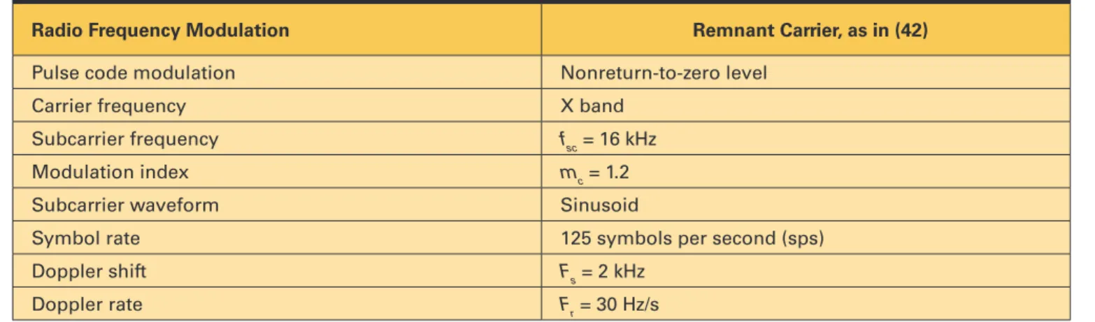
This study case considers the following telecommand transmit-ted (space-to-Earth) signal model known as remnant carrier modu-lation with sinusoidal subcarrier:
(
)
(
)
( ) sin 2 c c ( )sin 2 sc sc( ) c( ) ,
s t =A πf t m D t+ πf t+φ t +φ t (42)
with fc, fsc being the carrier or subcarrier frequencies, ϕc(t), ϕsc(t) the
carrier or subcarrier phase, mc the modulation index (0 < mc < π),
D(t) the information data stream, and A the signal amplitude, with D(t) = n ( s), n
n
c p t nT c− ∈
{+1,−1}, Ts symbol period and p(t) thepulse shape. The communication channel is modeled as an AWGN
Figure 7.
(a) ℜMSE obtained from 200 Monte Carlo runs for different carrier tracking techniques. Signal of interest corrupted by moderate and severe scintillation. Doppler frequency (b) and scintillation phase (c) estima-tion for one single realizaestima-tion, using a standard KF and the improved KF-Aℜ.
channel in the presence of Doppler and phase noise. The received signal is then given by
2 noise 1 2 2 ( ) , s k r k j F kT F kT k k k r x e π φ n + + = + (43)
where xk is the received digital baseband signal and Tk the sample
period. The Doppler shift and Doppler rate are denoted by Fs and
Fr, respectively. The phase noise ϕnoise is introduced at the simula-tion by applying a mask similar to the one defined in [76], and AWGN is added according to nk ∼ (0, N0).
To illustrate the potential application of KFs to this case study, the challenging carrier tracking scenario is evaluated by means of Monte Carlo simulations implementing the telecommand link specified in Table 1. Fig. 8a depicts the CP steady-state ℜMSE for both second- and third-order PLLs compared with a standard AKF-based tracking loop. The reference lock refers to the σ = 30° loss-of-lock rule-of-thumb [3]. The performance obtained with both PLLs is similar when considering the same loop bandwidth and slightly worse with the second-PLL with a higher bandwidth, as typically considered in the carrier acquisition stage. The perfor-mance gain obtained with the AKF is clear from the results, where for this specific case study the performance improvement is higher at lower Es/N0.
Fig. 8b illustrates the automatic adaptive bandwidth given by the AKF approach versus the constant standard PLL band-width (i.e., acquisition mode Bw = 20 Hz, tracking mode Bw = 10 Hz). When using the latter, the transition between acquisition and tracking modes is performed heuristically, while the adap-tive bandwidth provided by the AKF is based on the optimal filtering solution. Notice that the AKF bandwidth starts at 45 Hz for a fast acquisition and then converges to 7.5 Hz in the steady-state regime.
Although KF approaches can offer advantages over PLL con-figurations in terms of adaptability, further investigation with a more exhaustive analysis on its robustness and complexity require-ments for the very low SNℜ regime is needed.
Figure 8.
(a) CP ℜMSE versus different Es/N0 values at the input of the
demodu-lator for the 125 sps case. (b) Adaptive (KF) versus constant (PLL) bandwidth example.
Table 1.
Parameters of the Deep Space Telecommand Communication Link Used in the Simulations
Radio Frequency Modulation Remnant Carrier, as in (42)
Pulse code modulation Nonreturn-to-zero level
Carrier frequency X band
Subcarrier frequency fsc = 16 kHz
Modulation index mc = 1.2
Subcarrier waveform Sinusoid
Symbol rate 125 symbols per second (sps)
Doppler shift Fs = 2 kHz