HAL Id: hal-00646400
https://hal.inria.fr/hal-00646400
Submitted on 19 Feb 2013
HAL is a multi-disciplinary open access
archive for the deposit and dissemination of
sci-entific research documents, whether they are
pub-lished or not. The documents may come from
teaching and research institutions in France or
abroad, or from public or private research centers.
L’archive ouverte pluridisciplinaire HAL, est
destinée au dépôt et à la diffusion de documents
scientifiques de niveau recherche, publiés ou non,
émanant des établissements d’enseignement et de
recherche français ou étrangers, des laboratoires
publics ou privés.
Advanced Composition in Virtual Camera Control
Rafid Abdullah, Marc Christie, Guy Schofield, Christophe Lino, Patrick
Olivier
To cite this version:
Rafid Abdullah, Marc Christie, Guy Schofield, Christophe Lino, Patrick Olivier. Advanced
Com-position in Virtual Camera Control.
Smart Graphics, Aug 2011, Bremen, Germany.
pp.13-24,
�10.1007/978-3-642-22571-0_2�. �hal-00646400�
Advanced Composition in Virtual Camera
Control
R. Abdullah1, M. Christie2, G. Schofield1, C. Lino2, and P. Olivier1
1 School of Computing Science, Newcastle University, UK 2 INRIA Rennes - Bretagne Atlantique, France
Abstract. Rapid increase in the quality of 3D content coupled with the evolution of hardware rendering techniques urges the development of camera control systems that enable the application of aesthetic rules and conventions from visual media such as film and television. One of the most important problems in cinematography is that of composition, the precise placement of elements in shot. Researchers already consid-ered this problem, but mainly focused on basic compositional properties like size and framing. In this paper, we present a camera system that automatically configures the camera in order to satisfy advanced compo-sitional rules. We have selected a number of those rules and specified rat-ing functions for them, then usrat-ing optimisation we find the best possible camera configuration. Finally, for better results, we use image processing methods to rate the satisfaction of rules in shot.
1
Introduction
As the field of computer animation evolved, camera control has developed from the simple process of tracking an object to also tackle the aesthetic problems a cinematographer faces in reality. As Giors noted, the camera is the window through which the spectator interacts with the simulated world [7]. This means that not only the content of screen space becomes very important but also its aesthetic qualities, making composition a very important aspect of camera con-trol.
For practical purposes, we divide the problem of composition into two levels: the basic level in which simple properties like position, size, and framing are considered and the advanced level in which more generic, aesthetic rules from photography and cinematography are considered. The rule of thirds is a good example of advanced level composition.
We are developing a camera system that automatically adjusts a camera in order to satisfy certain compositional rules gleaned from photography and cin-ematography literature, namely, the rule of thirds, diagonal dominance, visual balance, and depth of field. We implement rating functions for these rules and use optimisation to find the best possible camera configuration. The rating functions depend on image processing, rather than geometrical approximation as imple-mented in most systems. Though it has the disadvantage of not being real, it has the advantage of being precise which is a requirement in composition.
We start by discussing the most relevant research in this area, focussing on approaches to composition in different applications. Then, we explain the com-position rules we have selected and how to rate them. Finally, we demonstrate the use of our system in rendering a scene from a well known film.
2
Background
Many previous approaches targeted composition, but most of them only handled basic compositional rules. Olivier et al. [14], in their CamPlan, utilised a set of relative and absolute composition properties to be applied on screen objects. All the properties realised in CamPlan are basic. Burelli et al. [4] defined a language to control the camera based on visual properties such as framing. They start by extracting feasible volumes in according to some of these properties and then search inside them using particle swarm optimisation. Like CamPlan, this approach lacks support of advanced composition rules.
Another limitation in previous approaches is the use of geometrical approxi-mation of objects for faster computation. In his photographic composition assis-tant, Bares [2] improves composition by applying transformations on the camera to shift and resize screen elements. However, the system depends on approximate bounding boxes which is often not sufficiently accurate. To alleviate this problem, Ranon et al. [16] developed a system to accurately measure the satisfaction of vi-sual properties and developed a language that enables the definition of different properties. The main shortcoming of their system is that it only evaluates the satisfaction of properties, rather than finding camera configurations satisfying them.
The final limitation that we are concerned about is that the methods used in previous work on composition either has limited applicability in computer graphics, or cannot be applied at all. For example, in Bares’s assistant, depending on restricted camera transformations rather than a full space search limits the application of the method to improving camera configurations rather than finding camera configurations.
In digital photography world, Banerjee et al. [1] described a method to apply the rule of thirds to photographs by shifting the main subject(s) in focus so that it lies on the closest power corner. The main subject(s) is detected using a wide shutter aperture that blurs objects out of focus. Besides the limitation of the method to only one object and one rule, the method cannot be applied in computer graphics. Similarly, Gooch et al. [8] applied the rule of thirds on a 3D object by projecting its silhouette on screen and matching it with a template. Again, the method is limited to one object only.
Liu et al. [12] addressed the problem of composition using cropping and re-targeting. After extracting salient regions and prominent lines, they use particle swarm optimisation [10] to find the coordinates of the cropping that maximise the aesthetic value of an image based on rule of thirds, diagonal dominance, and visual balance. Though it addresses advanced composition, it cannot be applied to computer graphics.
Our system is an attempt to address the main shortcomings of the approaches above, namely a) the lack of advanced composition rules b) the use of approxi-mate geometrical models, and finally c) the limited applicability.
3
Composition Rules
Although we implement basic composition rules in our system, our primary focus is on more advanced aesthetic conventions. We have explored some of the most important rules in the literature of photography and cinematography and selected the following for implementation because they have a clear impact on the results:
1. Rule of Thirds: The rule of thirds proposes that a useful starting point for any compositional grouping is to place the main subject of interest on any one of the four intersections (called the power corners) made by two equally spaced horizontal and vertical lines [17]. It also proposes that prominent lines of the shot should be aligned with the horizontal and vertical lines [9]. See figure 1a. Composition systems that have implemented this rule are [1, 2, 5, 8, 12].
2. Diagonal Dominance: The rule proposes that “diagonal arrangements of lines in a composition produces greater impression of vitality than either vertical or horizontal lines” [17]. For example, in figure 1b, the table is placed along the diagonal of the frame. A system that has implemented this rule is [12].
3. Visual Balance: The visual balance rule states that for an equilibrium state to be achieved, the visual elements should be distributed over the frame [17]. For example, in figure 1c, the poster in the top-left corner balance the weight of the man, the bottle, the cups, and other elements. Systems that have implemented this rule are [2, 12, 13].
4. Depth of Field: The depth of field rule is used to draw attention to the main subject of a scene by controlling the parameters of camera lens to keep the main subject sharp while blurring other elements. See figure 1d. Besides the advanced composition rules, it is also important to have a set of basic rules to help in controlling some of the elements of the frame. For this, we have implemented the following basic composition rules:
1. Framing Rule: This rule specifies that the frame surrounding a screen element should not go beyond the specified frame. This rule is useful when an element needs to be placed in a certain region of the frame. See figure 1e. Other systems that have implemented this rule is [3, 4, 11, 14].
2. Visibility Rule: This rule specifies that a minimum/maximum percentage of an element should be visible. For example, a case like that of figure 1f in which showing a character causes another character to be partially in view can be avoided by applying this rule on the character to the right. Other systems that have implemented this rule are [3, 4, 14].
3. Position Rule: This rule specifies that the centre of mass of an element should be placed on a certain position of the screen. Other systems that have implemented this rule are [4, 14].
4. Size Rule: This rule specifies that the size of a certain element should not be smaller than a certain minimum or larger than a certain maximum (specified by the user of the system). This rule is mainly useful to control the size of an element to ensure its size reflects its importance on the frame. Other systems that have implemented this rule are [3, 4, 14].
As different compositions need different rules, the rules are specified manu-ally. All rules take an object ID(s) as a parameter and some other parameters depending on the rule’s requirements. We refer the reader to section 5 for prac-tical examples.
(a) Rule of Thirds (b) Diagonal Dominance (c) Visual Balance
(d) Depth of Field (e) Framing Rule (f) Visibility Rule Fig. 1: Images illustrating composition rules
4
Rules Rating
The camera systems of many applications depend on methods specific to the geometry of the application only. However, our system is scene-independent, with the ability to impose many rules on many objects which makes the problem strongly non-linear. This, along with the aim of producing aesthetically-maximal results, suggests rating shots according to the satisfaction of rules and using
optimisation to solve for the best possible camera configuration. We found the optimisation method used by Burelli et al. [4] and Liu et al. [12], particle swarm optimisation, to be very efficient, so we use it. The rating of shot is described in this section.
4.1 Rendering Approach
Many approaches use geometrical approximation (e.g. bounding boxes) of scene objects to efficiently rate rules via closed form mathematical expressions [2, 4]. The downside of this approach is being inaccurate. To address this downside, we use the rendering approach. We render scene objects as an offline image and then process the resulting image to rate rules satisfaction for a certain camera configuration. The downside of the rendering approach is speed because of the time needed to render objects and process resulting images.
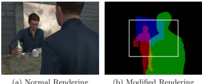
Since composition rules apply to certain objects only, which we call ruled ob-jects, we only render those objects and process the resulting image. However, one problem with image processing is the inaccuracy, difficulty, and cost of recognis-ing object extents in an image. Since for the rules we selected the most important aspect is the region occupied by an object rather than its colours, we can safely avoid these problems by rendering objects with unique distinct colour for each. Moreover, since the same pixel might be occupied by more than one object, the colour we use for each object occupies only one bit of the RGBA pixel, then using blending with addition we can have as many as 32 objects occupying the same pixel. The problem then comes down to comparing each pixel in the ren-dered image against objects’ colours. Figures 2a and 2b illustrates the modified rendering process.
An important issue to consider in the rendering method is that the resulting image tells nothing about the parts of an object which are out of view, making the rating of some rules incorrect, e.g. visibility rule. To solve this problem we use a field of view wider than the original such that the original view covers only the rectangle having corners (25%, 25%) and (75%, 75%), rather than the whole screen. This way we know which parts of objects are visible and which are invisible. This is illustrated in figure 2b in which the white rectangle represents the separator between the visible and invisible areas.
4.2 Rating Functions
In our system, each rule usually has several factors determining its rating value. For example, the rating of the diagonal dominance rule is determined by two factors: the angle between the prominent line of an object and the diagonal lines of the screen and the distance between the prominent line and the diagonal lines. For any rule, we rate each of its factors, then find the mean of ratings.
To get the best results from particle swarm optimisation, we suggest the following criteria for the rating of each factor:
(a) Normal Rendering (b) Modified Rendering
Fig. 2: To make image processing easier, we only render ruled objects and use different colour for each object. Furthermore, we bring the pixels resulting from the rendering towards the centre of the image such so that we can process pixels which are originally out of view.
1. While the function must evaluate to 1 when the factor is fully satisfied, it must not drop to 0, otherwise the method will be merely an undirected random search. However, after some point, which we call the drop-off point, the function should drop heavily to indicate the dissatisfaction of the factor. 2. The function must have some tolerance near the best value, at which the function will still have the value 1. This gives more flexibility to the solver. We suggest using Gaussian function as a good match for these criteria. For each factor, we decide a best value, a tolerance, and a drop-off value, and then use Gaussian function as follows:
F R= e(
∆ −∆t
∆do−∆t)2 (1)
where F R is factor rating, ∆ is the difference between the current value of the factor and the best value, ∆t is the tolerance of the factor, and ∆do is the
difference between the drop-off value and the best value.
Having the rating of each factor of a rule, we use geometric mean to find rule rating since it has the property of dropping down heavily if one of the factors drop heavily. However, the combined rating of all rules can be calculated using arithmetic or geometric mean (specified by the user) since sometimes it is not necessary to satisfy all rules. Moreover, weights can be specified for each rule according to its importance in the configuration.
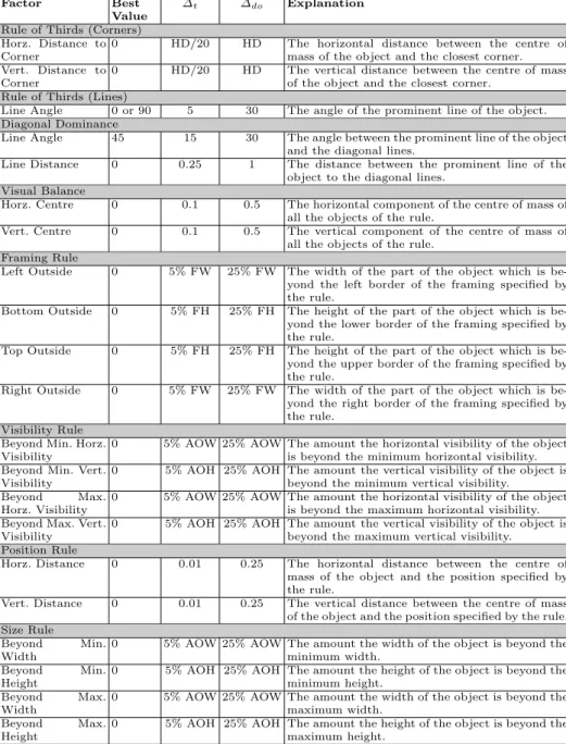
The data in table 1 gives the parameters of the different factors of all the composition rules we support in our system. Table 2 lists some of the symbols used in table 1. Crucially, we separate the rule of thirds into two rules, one for the power corners and the other for horizontal and vertical lines. This is because they usually apply to different elements of the screen.
4.3 Shot Processing
To rate the satisfaction of a rule we need to process the shot after rendering. The rating of framing rule and size rule depend on the frame surrounding the object
Factor Best Value
∆t ∆do Explanation
Rule of Thirds (Corners) Horz. Distance to Corner
0 HD/20 HD The horizontal distance between the centre of mass of the object and the closest corner. Vert. Distance to
Corner
0 HD/20 HD The vertical distance between the centre of mass of the object and the closest corner.
Rule of Thirds (Lines)
Line Angle 0 or 90 5 30 The angle of the prominent line of the object. Diagonal Dominance
Line Angle 45 15 30 The angle between the prominent line of the object and the diagonal lines.
Line Distance 0 0.25 1 The distance between the prominent line of the object to the diagonal lines.
Visual Balance
Horz. Centre 0 0.1 0.5 The horizontal component of the centre of mass of all the objects of the rule.
Vert. Centre 0 0.1 0.5 The vertical component of the centre of mass of all the objects of the rule.
Framing Rule
Left Outside 0 5% FW 25% FW The width of the part of the object which is be-yond the left border of the framing specified by the rule.
Bottom Outside 0 5% FH 25% FH The height of the part of the object which is be-yond the lower border of the framing specified by the rule.
Top Outside 0 5% FH 25% FH The height of the part of the object which is be-yond the upper border of the framing specified by the rule.
Right Outside 0 5% FW 25% FW The width of the part of the object which is be-yond the right border of the framing specified by the rule.
Visibility Rule Beyond Min. Horz. Visibility
0 5% AOW 25% AOW The amount the horizontal visibility of the object is beyond the minimum horizontal visibility. Beyond Min. Vert.
Visibility
0 5% AOH 25% AOH The amount the vertical visibility of the object is beyond the minimum vertical visibility.
Beyond Max. Horz. Visibility
0 5% AOW 25% AOW The amount the horizontal visibility of the object is beyond the maximum horizontal visibility. Beyond Max. Vert.
Visibility
0 5% AOH 25% AOH The amount the vertical visibility of the object is beyond the maximum vertical visibility.
Position Rule
Horz. Distance 0 0.01 0.25 The horizontal distance between the centre of mass of the object and the position specified by the rule.
Vert. Distance 0 0.01 0.25 The vertical distance between the centre of mass of the object and the position specified by the rule. Size Rule
Beyond Min. Width
0 5% AOW 25% AOW The amount the width of the object is beyond the minimum width.
Beyond Min. Height
0 5% AOH 25% AOH The amount the height of the object is beyond the minimum height.
Beyond Max. Width
0 5% AOW 25% AOW The amount the width of the object is beyond the maximum width.
Beyond Max. Height
0 5% AOH 25% AOH The amount the height of the object is beyond the maximum height.
Symbol Description
HD Half the distance between the power corners (i.e. 0.33333) FW Width of the frame used by the framing rule.
FH Height of the frame used by the framing rule.
AOW Average width of the projection on screen of the object being considered by a rule. AOH Average object of the projection on screen of the object being considered by a rule.
Table 2: Symbols and abbreviations used in factors calculation.
on screen which can be easily found. The rating of visibility rule depends on the number of pixels in the visible and invisible areas which is also straightforward to calculate. The rating of visual balance and the power corners in the rule of thirds, the rating depends on the centroid of the object, which is also straightforward to calculate.
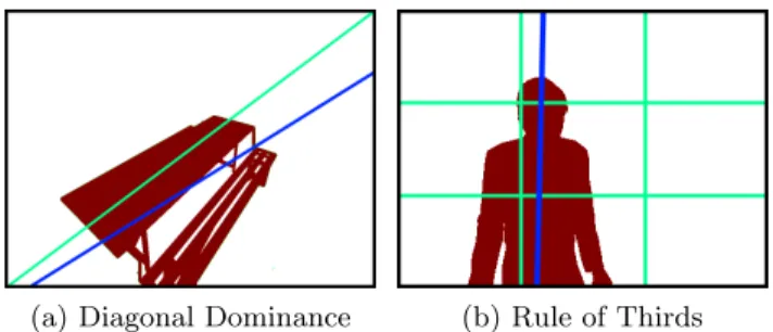
As for diagonal dominance and the horizontal and vertical lines in the rule of thirds, the rating depends on the prominent line of the ruled object, which is found by applying linear regression on the pixels of the object to find the best fitting line. The standard linear regression method works by minimising the vertical distance between the line and the points. This is mainly useful in case the aim of the regression is to minimise the error which is represented by the vertical distance between the line and the points. However, in our case we want to find a line that fits best rather than a line that minimises the error so we use a modified linear regression called perpendicular linear regression [18]. The method starts by finding the centroid of all the points then finding the angle of the line passing through the centroid which minimise the perpendicular distance. The angle is found according to the following equations:
tan(θ) = −A 2 ± r (A 2) 2− 1 (2) where A= Pn i=1x2i − Pn i=1yi2 Pn i=1xiyi (3) where (xi, yi) is the coordinate of the ith pixel of the object. Figure 3a illustrates
the prominent line of the table in figure 1b and figure 3b illustrates the same concept but for a character to be positioned according to rule of thirds.
Finally, the rating of the depth of field rule is always 1, as the adjustment of the camera lens cannot be decided before the position, orientation, and field of view of the camera are found. Once they are found, the camera depth of field are adjusted according to the size of the object and its distance from the camera.
5
Evaluation
As a practical demonstration of our system, we decided to render a scene from Michael Radford’s Nineteen Eighty-Four. The scene we selected is set in a can-teen and revolves around 4 important characters in the plot, Smith, Syme, Par-sons, and Julia. In the scene, the protagonist, Smith is engaged in conversation
(a) Diagonal Dominance (b) Rule of Thirds
Fig. 3: Illustrating how the prominent line of an object is found using perpen-dicular linear regression. The line in blue is the prominent line extracted from the object in dark red.
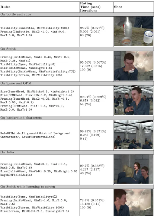
with Syme and Parsons at the lunch table, and Julia is watching Smith from across the room. An additional secondary character participates briefly in one of the conversations and we call him OPM (abbreviation of Outer Party Member). The scene has been rendered in 3DSMAX and exported to OGRE. We used our system to automatically find camera configurations that show shots similar to those of the original scene. We then used those camera configurations to generate a video of the rendering of the scene. The video is attached with this paper. Table 3 lists some of the shots that have been generated and the rules used to generate each shot. For each shot, we repeated the test 10 times and calculated the mean and standard deviation of the achieved rating, processing time, and number of iterations until a solution is found, which we also include in the table in the second column, where the standard deviation is the value in brackets. Finally, our screen coordinates range from (-1, -1) at the bottom-left corner to (1, 1) at the top-right corner.
The system we ran the test on has a 2.66 GHz Intel Core 2 Quad Core Q9400 processor and an NVIDIA GeForce 9800 GT video card with 512 MB of video memory. For the rating, scene objects are rendered on an 128×128 offline texture. It is possible to use smaller texture sizes to reduce processing time, but this will decrease the accuracy of the results.
We configured the PSO to use 36 particles in each iteration, each particle representing a camera configuration of 3D position, 2 orientation angles, and an angle for the field of view. Initially, the position is randomly positioned in boxes manually specified around the objects of interest. The orientation and field of view angles are also randomly specified in a manually set range. The algorithm breaks if the rating reach 98% or after 100 iterations. As obvious from the table data, the standard deviation of the rating is either zero or negligible, which shows that the results obtained by the system are steady. Another thing to notice is that the processing time varies widely among the different shots because different shots have different rules. Also, the standard deviation of the time is relatively large because, depending on the initial random configurations,
the required number of iterations before a solution is reached varies widely. In the fourth configuration specifically, the number of iterations is zero. This is because we fixed the position of the camera to Syme’s eyes to show the view from his perspective, and only allowed the camera pitch and field of view to be adjusted, making it enough for the initial step to find a satisfactory solution. Finally, the rating of the last shot is relatively low because the used rules cannot be satisfied together.
Finally, the number of particles used has an important effect on the result. For in one hand, if we reduce the number of particles, the achieved rating will decrease, while if we increase the number of particles, the processing time will heavily increase with not much gain in rating. For more information about tuning particle swarm optimisation we refer the reader to [6, 15].
6
Conclusion and Future Work
We have implemented a camera system for advanced composition. The system has been implemented based on particle swarm optimisation, which proved to be very successful in finding solutions in high dimensional search spaces, a neces-sity for camera control. To get accurate results we rated shots based on image processing, as opposed to geometric approximation. The main shortcoming of our approach is the time it takes to find a solution, which makes the system limited to offline processing only. The other shortcoming is that the occlusion problem is not considered here as it requires full rendering of the scene which is a expensive operation. Future work will be focused on solving these two shortcom-ings. We are investigating the possibility of implementing the image processing computations on the GPU rather than the CPU. This would heavily reduce the processing time, as the bottleneck of our system is transferring the image data from the GPU memory and processing them in the CPU.
7
Acknowledgements
This research is part of the “Integrating Research in Interactive Storytelling (IRIS)” project, and we would like to thank the European Commission for fund-ing it. We would also like to forward our thanks to Zaid Abdulla, from the American University of Iraq Sulaimani (AUI-S) for his invaluable help with the technical aspects of the research. Finally, we would like to thank the reviewers of this paper for their comments.
Rules
Rating Time (secs) Iterations
Shot On bottle and cups
Visibility(GinBottle, MinVisibility:100%) Framing(GinBottle, MinX:-1.0, MinY:0.0, MaxX:0.0, MaxY:1.0)
98.2% (0.077%) 5.006 (2.061) 63 (26)
On Smith
Framing(Smith#Head, MinX:-0.43, MinY:-0.6, MaxX:0.36, MaxY:1) Visibility(Syme, MaxVisibility:0) Size(Smith#Head, MinHeight:1.6) Visibility(Smith#Head, MinVertVisibility:70%) Visibility(Screen, MinVisibility:70%) 95.56% (0.567%) 17.352 (0.515) 100 (0)
On Syme and OPM
Size(Syme#Head, MinWidth:0.5, MinHeight:1.2) Size(OPM#Head, MinWidth:0.2, MinHeight:0.4) Framing(Syme#Head, MinX:-0.05, MinY:-0.5, MaxX:0.55, MaxY:0.9)
Framing(OPM#Head, MinX:-0.4, MinY:0.0, MaxX:0.0, MaxY:1.0)
99.01% (0.669%) 6.878 (3.032) 54 (24)
On background characters
RuleOfThirds Alignment(<List of Background Characters>, LowerHorizontalLine)
99.43% (0.371%) 0.285 (0.129) 0 (1)
On Julia
Framing(Julia#Head, MinX:0.0, MinY:-0.1, MaxX:0.5, MaxY:0.6)
Size(Julia#Head, MinWidth:0.25, MinHeight:0.5) DepthOfField(Julia)
99.7% (0.368%) 4.237 (2.137) 48 (24)
On Smith while listening to screen Visibility(Syme, MaxVisibility:0%) Framing(Smith#Head, MinX:-1.0, MinY:0.0, MaxX:0.5)
Visibility(Screen, MinVisibility:100%) Size(Screen, MinWidth:2.5, MinHeight:2.5)
72.4% (0.351%) 15.188 (0.11) 100 (0)
Table 3: The list of shots used in the rendering of a scene from Nineteen Eighty-Four. For each shot, we repeated the test 10 times and calculated the average rating the system could achieve and the average time spent in the solving process. The numbers in the brackets are the standard deviation of the results of the 10 tests.
References
1. Banerjee, S., Evans, B.L.: Unsupervised automation of photographic composition rules in digital still cameras. In: In Proceedings of SPIE Conference on Sensors, Color, Cameras, and Systems for Digital Photography. vol. 5301, pp. 364–373 (2004)
2. Bares, W.: A photographic composition assistant for intelligent virtual 3d cam-era systems. In: Smart Graphics, Lecture Notes in Computer Science, vol. 4073, chap. 16, pp. 172–183–183. Springer Berlin / Heidelberg, Berlin, Heidelberg (2006) 3. Bares, W., McDermott, S., Boudreaux, C., Thainimit, S.: Virtual 3D Camera Com-position from Frame Constraints. In: Proceedings of the eighth ACM international conference on Multimedia. pp. 177–186. ACM (2000)
4. Burelli, P., Gaspero, L., Ermetici, A., Ranon, R.: Virtual camera composition with particle swarm optimization. In: Proceedings of the 9th international symposium on Smart Graphics. pp. 130–141. SG ’08, Springer-Verlag, Berlin, Heidelberg (2008) 5. Byers, Z., Dixon, M., Smart, W.D., Grimm, C.M.: Say Cheese! Experiences with
a Robot Photographer. AI Magazine 25(3), 37 (2004)
6. Carlisle, A., Dozier, G.: An off-the-shelf pso. In: Proceedings of the Workshop on Particle Swarm Optimization. vol. 1, pp. 1–6 (2001)
7. Giors, J.: The full spectrum warrior camera system (2004)
8. Gooch, B., Reinhard, E., Moulding, C., Shirley, P.: Artistic composition for image creation. In: Eurographics Workshop on Rendering. pp. 83–88 (2001)
9. Grill, T., Scanlon, M.: Photographic Composition. Amphoto Books (1990) 10. Kennedy, J., Eberhart, R.C.: Particle swarm optimization. In: Proceedings of the
IEEE International Conference on Neural Networks. pp. 1942–1948 (1995) 11. Lino, C., Christie, M., Lamarche, F., Schofield, G., Olivier, P.: A Real-time
Cin-ematography System for Interactive 3D Environments. In: Proceedings of the 2010 ACM SIGGRAPH/Eurographics Symposium on Computer Animation (SCA) (July 2010)
12. Liu, L., Chen, R., Wolf, L., Cohen-Or, D.: Optimizing photo composition. Com-puter Graphic Forum (Proceedings of Eurographics) 29(2), 469–478 (2010) 13. Lok, S., Feiner, S., Ngai, G.: Evaluation of Visual Balance for Automated Layout.
In: Proceedings of the 9th international conference on Intelligent user interfaces. pp. 101–108. ACM (2004)
14. Olivier, P., Halper, N., Pickering, J., Luna, P.: Visual composition as optimisation. In: AISB Symposium on AI and Creativity in Entertainment and Visual Art. pp. 22–30 (1999)
15. Pedersen, M.E.H.: Tuning & Simplifying Heuristical Optimization (PhD Thesis). sl: School of Engineering Sciences. Ph.D. thesis, University of Southampton, United Kingdom (2010)
16. Ranon, R., Christie, M., Urli, T.: Accurately measuring the satisfaction of vi-sual properties in virtual camera control. In: Taylor, R., Boulanger, P., Krger, A., Olivier, P. (eds.) Smart Graphics, Lecture Notes in Computer Science, vol. 6133, pp. 91–102. Springer Berlin / Heidelberg (2010)
17. Ward, P.: Picture Composition for Film and Television. Focal Press (2003) 18. Weisstein, E.W.: Least squares fitting–perpendicular offsets.
http://mathworld.wolfram.com/LeastSquaresFittingPerpendicularOffsets.html (2010)
![[PDF] Tutoriel pour Apprendre à programmer en ActionScript 3 | Cours informatique](data:image/gif;base64,R0lGODlhAQABAIAAAP///wAAACH5BAEAAAAALAAAAAABAAEAAAICRAEAOw==)