Actuation Efficiency and Work Flow in piezoelectrically Driven
Linear and Non-linear Systems
by
Yong Shi
B. Eng., National University of Defense Technology, P. R. China (1985)
Submitted to the Department of Aeronautics and Astronautics
in partial fulfillment of the requirements for the degree of
Master of Science
at the
MASSACHUSETTS INSTITUTE OF TECHNOLOGY
June 2001
@
Massachusetts Institute of Technology 2001. All rights reserved.
The author hereby grants to MASSACHUSETTS INSTITUTE OF TECHNOLOGY
permission to reproduce and
to distribute copies of this thesis document in whole or in part.
Signature of Author...
-T
-.. .. . .. . .. . . ...Department of Aeronautics and Astronautics
2 May 2001
Certified by...
...----
-
-
---Nesbitt W. Hagood, IV
Associate Professor, Thesis Supervisor
Thesis Supervisor
Accepted by... ...
Wallace E. Vander Velde
MASSACHUSETTS INSTITUTE Professor of Aeronautics and Astronautics
OF TECHNOLOGY
OEC
11 - 2 001Chair,
Committee on Graduate StudentsSEPR1RE001
Actuation Efficiency and Work Flow in piezoelectrically Driven Linear and
Non-linear Systems
by
Yong Shi
Submitted to the Department of Aeronautics and Astronautics on 2 May 2001, in partial fulfillment of the
requirements for the degree of Master of Science
Abstract
It is generally believed that the maximum actuation efficiency of piezoelectrically driven systems is a quarter of the material coupling coefficient squared. This maximum value is reached when the stiffness ratio of structure and piezo stack equals to one. However, previous study indicts that load coupling has significant influence on the work flow and actuation efficiency in the systems. Theoretical coupled analysis of such systems has shown that the actuation efficiency is the highest at the stiffness ratio larger than one and this maximum value is much higher than that predicted by the uncoupled analysis when coupling coefficient is relatively high. Moreover, for non-linear systems, the actuation efficiency can be twice as high as that of linear systems. The objectives of this research is to verify the theoretical coupled analysis experimentally and explore the possibility for the mechanical work to be done into the environment. To do this, a testing facility has been designed and built with programmable impedances and closed loop test capability. However, the feedback control method is not fast enough in determining the voltage for the driving stack which has limited the test frequency. Meanwhile, the original mechanical design can not guarantee the accurate measurement of mechanical work. Renovation on the existing tester has been made and feed forward open loop test methodology has been used utilizing a Force-Voltage model developed from Ritz Formulation. Linear test results correlate very well with the theoretical prediction. Two linear functions have been chosen for non-linear tests. The results have shown that the actuation efficiency of non-non-linear systems is much higher than that of linear systems. The actuation efficiency of system simulated by non-linear function 1 is about 200% that of linear systems and the work output of this system is about 254% that of the linear systems. These test results exactly proved out the theoretical prediction of non-linear loading systems. The capability of modeling and testing of non-conservative thermodynamic cycles have also been demonstrated which make it possible to take advantage
of the mechanical work out of the systems.
Thesis Supervisor: Nesbitt W. Hagood, IV Title: Associate Professor, Thesis Supervisor
Acknowledgements
It is with heartfelt gratitude that I dedicate this thesis to all those who have played a role in the successful completion of my research. I would like to thank Ching-Yu Lin, David Roberson, Mauro Atlalla, Chris Dunn, Viresh Wickramasinghe, Timothy Glenn as well as all my lab-mates and roommates who are always ready to help me in every expect from the tester design, test setup, data acquisition and handling, signal analysis and the using of different equipment or instrument and software in the lab, just to mention a few. Their sincere helps make my research a lot easier and my working at AMSL a wonderful memory.
I am also very grateful to my Chinese friends here and I would also like to thank my family-my parents, family-my wife, family-my brother and sisters. I am very grateful to family-my parents who love me and worry about me all the time. My special thanks go to my wife Zhihong. It is her love which actually makes all this becoming true. I still remember all the sufferings in the past two years, the pain from legs and the pain from research. She is always standing by my side taking care of me and encouraging me. There is no word which could express my love and thanks to her. I would also like to dedicate this thesis to my son-Caleb who will come to this word very soon. Funding for this research was provided by the Office of Naval Research (ONR) Young Investigator's Program. under contract N00014-1-0691, and monitored by Wallace Smith.
Nomenclature
a Stiffness ratio, load stiffness divided by material stiffnes A Cross-sectional area of the material
A, Cross-sectional area of the piezoelectric material, or the sample stack
Ap2 Cross-sectional area of the driving stack
As Cross-sectional area of the structure
CP5. Capacitance of the system under constant strain
E Young's modulus of the active material in the "three-three" direction under
constant electric field
Co Linear part of the Young's modulus of non-linear loads
cS Young's modulus of the structure
cX Non-linear part of the Young's modulus of non-linear loads
6 Variation operator
d Derivative operator
D3 Electric displacement in the active material in the "three" direction
d33 Electromechanical coupling term of the active material in the "three-three" direction
60 Dielectric constant of free space
e3 Dielectric constant of the active material in the "three-three" direction under constant strain
3 Dielectric constant of the active material in the "three-three" direction 33
E3 et e33
fi
f2 FbI Finear Finear Fnon-lineari Fnon-linear2f,
K, E 1 ks k33l1
lP1 77max N 01 02Qi
Q2 S3 sES 3 3Electric field in the active material in the "three" direction Electromechanical coupling of active materials
Electromechanical coupling of active materials in the "three-three" direction Generalized force vector of the active material of the sample stack
Generalized force vector of the driving stack Blocked the force of the active material Blocked the force of the active material Linear Load
Non-linear load 1 Non-linear load 2
Generalized force vector of the structure
Stiffness of the active material under constant electric field Stiffness of the structure
Material coupling coefficient of the active material Length of material or structure
Length of active material Length of structure
Actuation efficiency of systems
Maximum actuation efficiency of systems Number of layers in piezoelectric stack
Electromechanical coupling of the active material Electromechanical coupling of the driving stack
Charge vector of the active material Charge vector of the driving stack
Strain in "three" direction of the active material
Elastic constant of the active material in the "three-three" direction under constant electric field
D
S3 3 Elastic constant of the active material in the "three-three" direction at
open circuit
Elastic constant of the active material in the "three-three" direction at open circuit
Thickness of the stack layers Initial voltage to the sample stack
Voltage applied to the active material or the sample stack during testing Voltage applied to the driving stack
Final voltage to the sample stack Maximum voltage applied during tests
Volume of the active material or the sample stack Electric Work
Mechanical work Work into the system Work out of the system Initial displacement
Displacement of the system
Displacement of the active materials Displacement of the driving stack Free displacement of the system Electric mode shape
Mechanical mode shape
ti V V1 V2 Vf Vmax VP1i WE WM Win Wout Xo x1 x2 Xfree or Xf XFE Wu M
Contents
1 Introduction
1.1 Motivation . . . . 1.2 O bjective . . . .
1.3 Previous Work . . . .
1.3.1 Material Coupling Coefficient. . . . .
1.3.2 Berlincount's Work . . . .
1.3.3 Lesieutre and Davis' Work . . . .
1.3.4 Spangler and Hall's Work . . . .
1.3.5 Giurgiutiu's Work . . . .
1.3.6 C. L. Davis' Work . . . . 1.3.7 M. Mitrovic's Work . . . . 1.3.8 Malinda and Hagood's Work . . . . 1.4 A pproach . . . .
1.5 Organization of the Document . . . .
2 Analysis of the Work Flow and Actuation Efficiency Coupled Systems
2.1 Definition of Work Terms . . . . 2.1.1 Mechanical Work . . . . 2.1.2 Electrical Work . . . .
2.1.3 Actuation Efficiency . . . .
2.2 Linear and Non-linear Systems . . . .
16 16 17 . . . 17 . . . 17 . . . 18 . . . 18 . . . . 19 . . . 20 . . . 21 . . . 21 . . . 22 . . . 23 . . . 24 of Electromechanically 26 27 28 28 28 29
2.3 General Analysis . . . . 30
2.3.1 Linear Constitutive Equations . . . . 31
2.3.2 Governing Equations for the coupled systems . . . 31
2.3.3 Compatibility and Equilibrium . . . 32
2.3.4 Electrical Work . . . 32
2.3.5 Mechanical Work . . . 33
2.3.6 Actuation Efficiency . . . . 33
2.4 One Dimensional Linear Systems . . . . 34
2.4.1 Expressions for Linear Systems . . . . 34
2.4.2 Constitutive Equations . . . . 34
2.4.3 Finding the Constants in Work Expressions . . . . 35
2.4.4 Simplified Expressions for Electrical and Mechanical Work . . . . 36
2.4.5 Actuation Efficiency . . . . 37
2.4.6 Discussion on Actuation Efficiency . . . . 37
2.5 One dimensional Non-linear Systems . . . . 38
2.5.1 General Analysis . . . . 38
2.5.2 Mechanical and electrical Work in terms of Displacement . . . . 39
2.5.3 Simplified Expressions for Mechanical and Electrical Work . . . . 40
2.5.4 Actuation Efficiency . . . . 41
2.6 Comparison of Linear and Non-linear Systems . . . . 41
2.7 Summary . . . . 43
3 Renovation on the Existing Component Testing Facility 44 3.1 The existing Component Tester . . . . 44
3.1.1 Design Requirements . . . . 44
3.1.2 Main Features of the Component Tester . . . . 45
3.2 Previous Test Results . . . . 46
3.2.1 Material Properties Measurement . . . . 46
3.2.2 Linear Test Results . . . . 47
3.2.3 Nonlinear Test Results . . . . 47
3.3.1 Electrical Work Measurement . . . .
3.3.2 Mechanical Work Measurement . . . .
3.4 Re-design of the Load Transfer Device . . . . 3.4.1 Initial design . . . . 3.4.2 Vibration Measurement and Improvement
3.5 Validation of the New Design . . . .
3.5.1 Stiffness Measurement . . . .
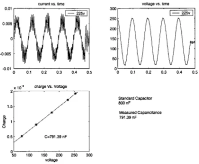
3.5.2 Capacitance Measurement . . . .
3.6 Sum m ary . . . .
4 One Dimensional Linear and Non-linear Tests 4.1 FeedBack Test Approach . . . . 4.2 FeedForward Test Approach . . . . 4.3 Material Properties of Test sample . . . . 4.3.1 Test Sample Physical Parameters . . . .
4.3.2 Stiffness and Elastic Constants . . . . . 4.3.3 Capacitance and Dielectric Constant . . 4.3.4 Electromechanical Coupling Term . . .
4.3.5 Material Coupling Coefficient . . . . 4.3.6 Material Properties Summary . . . . 4.4 Actuating Voltage for Test Sample . . . . 4.4.1 Linear and non-linear Functions . . . .
4.4.2 Actuating Voltage for Sumitomo Stack . 4.5 Voltage-Force Model . . . . 4.5.1 Model Development . . . . 4.6 4.7 4.8 . . . 5 0 . . . 5 1 . . . 5 5 . . . 5 5 on the Design . . . . 56 . . . 6 2 . . . 6 2 . . . 6 5 . . . 6 6 68 . . . 6 8 . . . 7 1 . . . 7 1 . . . 7 1 . . . 7 3 . . . 7 4 . . . 7 6 . . . 7 7 . . . 7 9 . . . 8 0 . . . 8 0 . . . 8 0
4.5.2 Experimental Determination of model coefficients . . . .
Theoretical Predictions for systems driven by Sumitomo Stack Linear Tests . . . . Non-linear Tests . . . . 4.8.1 Non-linear system 1 . . . . 4.8.2 Non-linear system 2 . . . . 83 83 85 87 89 90 95 96
4.9 Com parison and Discussion . . . . 4.10 Sum m ary . . . .
5 Non-Conservative Systems
5.1 Net Work in Conservative Systems . . . . .
5.2 Non-Conservative System and Its Efficiency
5.2.1 Non-Conservative Cycles . . . . 5.2.2 Efficiency . . . . 5.3 Experimental Demonstration . . . . 5.3.1 Simulation Methods . . . . 5.3.2 Test Results . . . . 5.4 Summ ary . . . .
6 Conclusions and Recommendations for Future Work
6.1 Conclusions on Linear and Non-linear Tests . . . .
6.2 Conclusions on Non-Conservative Systems . . . .
6.3 Recommendation for Future Work . . . .
A Component Testing Facility Drawings
. . . 101 . . . 106 108 . . . 1 0 8 . . . 1 0 8 . . . 1 0 8 . . . 1 1 0 . . . 1 1 0 . . . 1 1 0 . . . 1 1 0 . . . 1 1 5 117 117 118 119 123
List of Figures
2-1 Piezoelectrically Driven One Dimensional Model . . . .
2-2 Material and Structure Loading Line for the Linear Systems . . . .
2-3 Comparison of Linear and Non-linear Functions . . . . 2-4 Comparison of Actuation Efficiency of Linear Systems with Different k33 . . .
2-5 Max. Actuation Efficiency vs. k33 for ID Linear Systems . . . .
2-6 Comparison of Electrical and Mechanical Work for 1D Systems . . . .
2-7 Comparison of Actuation Efficiency for 1D systems . . . .
The Original Component Testing Facility . . . . Determination of k3 3 for Sumitomo Stack . . . .
Mechanical Work vs. Stiffness Ratio a for Linear Systems . . Electrical Work vs. Stiffness Ratio a for Linear Systems . . .
Actuation Efficiency vs. Stiffness Ratio a for Linear Systems Comparison of Actuation Efficiency for Linear and Non-linear Time Trace of from Previous Test . . . . Stiffness of PETI-1 vs. Applied Preload . . . . The Original Alignment Mechanism . . . .
Stiffness of the Alignment Mechanism vs.Preload . . . . The Original Cage System for Load Transfer and Protection . New Design of the Load Transfer System . . . .
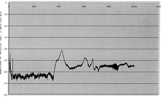
Transfer Function of the Transverse Velocity of Test Sample to Transverse Vibraton of Test Sample at Time 1 . . . . Transverse Vibration at Time 2 . . . .
Systems
the Input to Drive 27 29 30 38 39 42 42 45 47 48 48 49 50 51 53 53 54 55 57 57 58 58 3-1 3-2 3-3 3-4 3-5 3-6 3-7 3-8 3-9 3-10 3-11 3-12 3-13 3-14 3-15
3-16 Transverse Vibration at Time 3 . . . . 3-17 Transverse Vibration at Time 4 . . . . 3-18 Transverse Vibration at Time 5 . . . . 3-19 Transverse Vibration at Time 6 . . . .
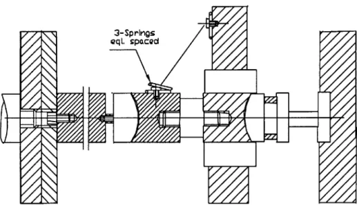
3-20 Improvement on the New Design by Providing Springs for Preload . . .
3-21 New Design of the Load Transfer Systemsl . . . .
3-22 New Design of the Load Transfer System 2 . . . .
3-23 Overall View of the New Tester . . . .
3-24 Force Calibration for the New Design . . . .
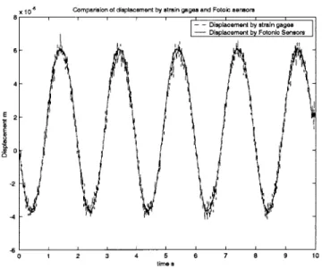
3-25 Comparison of Displacement measured by Two MTI Probes . . . .
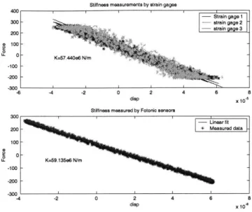
3-26 Comparison of Displacement Measured by MTI Probes and Strain Gages 3-27 Stiffness Measured from MTI probes and Strain Gages . . . .
3-28 Capacitance Measurement for Standard Capacitor . . . .
4-1 4-2 4-3 4-4 4-5 4-6 4-7 4-8 4-9 4-10 4-11 4-12 4-13 4-14 4-15 4-16 4-17
Time Trace for Linear Test at 0.05 Hz, Assumed Stiffness 3000 lbs/in . .
Time Trace for Linear Test at 1 Hz, Assumed Stiffness 3000 lbs/in . . . .
Time Trace for Linear Test at 10 Hz, Assumed stiffness 3000 lbs/in . . . .
Feedforward Open Loop Test Approach . . . . Time Trace of Displacement and Force for Stack Stiffness Measurement Force vs. Displacement for Stack Stiffness Measurement . . . .
Time Trace of Current and Voltage for Capacitance Measurement . . . . . Charge vs. Volatge for Capacitance Measurement . . . . Time Trace of Displacement and Voltage for Stack d33 Measurement . . . Displacement vs. Voltage for Stack d3 3 Measurement . . . . Linear and Non-linear Functions in terms of Displacement of the Actuator Voltage vs. Displacement from Coupled Analysis . . . . Three Component System for Voltage-Force Model . . . . Force vs. Voltage V1 for Voltage-Force Model . . . . Force vs. Voltage VI and V2 for Voltage-Force Model . . . . Prediction of Mechanical Work for Systems Driven by Sumitomom Satck. Prediction of Electrical Work for Systems Driven by Sumitomo Satck . .
. . . . 59 . . . . 59 . . . . 59 . . . . 59 . . . . 60 . . . . 61 . . . . 61 . . . . 62 . . . . 63 . . . . 64 . . . . 64 . . . . 65 . . . . 66 . . . . 69 . . . . 70 . . . . 70 . . . . 72 . . . . 75 . . . . 75 . . . . 76 . . . . 77 . . . . 78 . . . . 79 . . . . 81 . . . . 83 . . . . 84 . . . . 87 . . . . 87 . . . . 88 . . . . 89
4-18 4-19 4-20 4-21 4-22 4-23 4-24 4-25 4-26
Prediction of Actuation Efficiency for Systems Driven by Sumitomo Satck . . Typical Displacement Measurement for Linear Tests . . . . Typical Force Measurement for Linear Tests . . . . Typical Current and Voltage Measurement for Linear Tests . . . . The Resentative Cycle for Computing Work Terms . . . . Typical Effective Stiffness Determined from Actaul Data . . . . Typical Mechanical Work from Theory and Experiment for Linear Test . . .
Typical Electrical Work from Theory and Experiment for Linear Tests . . . .
Actuation Efficiency as a Function of Stiffness Rato Ks/K3 for Linear Tests
. . 89 . . 91 . . 92 . . 92 . . 93 . . 93 . . 94 . . 94 . . 95
4-27 Predicted Displacement and Force for Non-linear Test 1 . . . 96
4-28 Predicted Voltage to the Driving Stack for Non-linear Test 1 . . . 97
4-29 Measured Displacement of Sample for Non-linear System 1 . . . 97
4-30 Measured Force in the System for Non-linear System 1 . . . 98
4-31 Measured Volatge and Current for Non-linear Test 1 . . . 98
4-32 Representative Cycle for Work terms for Non-linear 1 . . . 99
4-33 Simulated Force vs. Displacement for Non-linearl . . . . 99
4-34 Mechanical Work out Comparison for Non-linear System 1 . . . 100
4-35 Electrical Work in Comparison for Non-linear System 1 . . . 100
4-36 Predicted Force and Displacement for Non-linear 2 . . . 101
4-37 Computed Voltage to Driving Stack for Non-liner 2 . . . 102
4-38 Measured Displacement of Sample for Non-linear System 2 . . . 102
4-39 Measured Force in the system for Non-linear System 2 . . . 103
4-40 Measured Current and Voltage for Non-linear System 2 . . . 103
4-41 Representative Cycle for determining Work Terms for non-linear 2 . . . 104
4-42 Simulated Force vs. Displacement for Non-linear System 2 . . . 104
4-43 Mechanical Work out Comparison for Non-linear system 2 . . . 105
4-44 Electrical Work in Comparison for Non-linear system 2 . . . 105
4-45 Comparison of Mechanical Work for Linear and Non-linear Systems . . . 106
4-46 Comparison of Electrical Work for Linear and Non-linear Systems . . . 107
5-2 5-3 5-4 5-5 5-6 5-7 5-8 5-9 5-10 5-11 5-12 A-1 A-2 A-3 A-4 A-5 A-6 A-7 A-8 A-9
Assembly Drawing of the Renovated Component Tester Adaptor 2 Drawing . . . . Adaptor 6 Drawing . . . . Adaptor 7 Drawing . . . .
Adaptor 9 Drawing . . . . Linear Bearing Mounting Plate Drwaing . . . . Adaptor 3 Drawing . . . . Adaptor 4 Drawing . . . . Adaptor 5 Drawing . . . .
Different Non-Conservative Thermodynamic Cycles . . . . Voltage to the Sample and Driving Stacks . . . . Displacement Measurement for a Non-Conservative Cycle . . . . Force Measurement for a Non-Conservative Cycle . . . . Current and Voltage Measurement for a Non-Conservative Cycle . . . .
Representative Cycle for Determining Work and Efficiency . . . .
Comparison of the Non-Conservative Cycle 1 and the Actually Simulated Net Mechanical Work Done by a Non-Conservative Cycle . . . . Net Electrical Work into a Non-Conservative Cycle . . . . Mechanical work and electric work vs. Sstress on the sample stack . . .
Efficiency of non-conservative cycles vs. stress on the sample stack . . .
. . . 124 . . . 125 . . . 126 . . . 127 . . . 128 . . . 129 . . . 130 . . . 131 . . . 132 . . . 109 . . . 111 . . . 111 . . . 112 .. .. 112 .. .. 113 Cycle 113 . . . 114 . . . 114 . . . 115 . . . 116
List of Tables
Driving Stack Parameters . . . . Sumitomo Stack Parameters . . . .
Al Bar Stiffness Measurement . . . .
Sumitomo Stack Physical Parameters . . . . Sumitomo Measured Stiffness at open Circuit . . . . ..
Sumitomo Stack Measured Compliance st Open Circuit . . . .
Sumitomo Stack Measured Stiffness at Short Circuit . . . . Sumitomo Stack Measured Compliance at Short Ciucuit . . . . Measured Capacitance and Dielectric Constant for Sumitomo Stack. . The Measured Material Properties for Sumitomo Stack . . . . Comparison of Actuation Efficiency for Linear and Non-linear Systems
46 47 . . . . 52 . . . 72 . . . 74 . . . 74 . . . 74 . . . 74 . . . 77 . . . 80 . . . 106 3.1 3.2 3.3 4.1 4.2 4.3 4.4 4.5 4.6 4.7 4.8
Chapter 1
Introduction
1.1
Motivation
Recently piezoelectric actuators have been extensively used for different applications, such as, precise positioning[Karl, 2000] and [Roberts, 1999], vibration suppression[Hagood, 1991] and [Binghamand, 1999], and ultrasonic motors [Bar-Cohen, 1999] and [Frank, 1999, spie]. More-over, their special characteristics have also made them popular in micro-systems as well as in optical device applications [Varadan, 2000, spie]. However, to use these actuators efficiently, it is necessary to evaluate and understand the material response, energy flow and actuation efficiency in the system at working conditions.
Piezoelectric materials have been initially developed for sensors applications initially which focus on low power properties. For example, the linear material model is valid for low electric field. These properties are not appropriate for the applications of actuators which are used at high frequency, high electric field, and high mechanical loads. Furthermore, standard as-sumptions about the efficiency of piezoelectrically driven systems neglect the electromechanical coupling in the system. These pending problems also necessitate the study of work flow and
1.2
Objective
The objective of this research is to closely examine the work input, work output and actuation efficiency in a fully coupled system. Different expressions such as material coupling coefficient, device coupling coefficient, and efficiency of coupling elements have been used traditionally to describe the systems. Actuation efficiency, which is a thermodynamic efficiency expression defined by the ratio of mechanical work out and electrical work in, may best describe coupled systems.
Previous theoretical analysis [Malindal, 1999] has shown that the actuation efficiency of one dimensional linear systems reaches the highest when the stiffness ratio of the structure and the active material is larger than one. This peak value of actuation efficiency is much higher than the prediction of the coupling element efficiency of Hall [Hall, 1996]when the coupling coefficient is relatively high. However, for active materials working against non-linear loads, it is possible to significantly increase the actuation efficiency in the systems. So another objective of this research is to validate the theoretical derivation and verify the analysis results experimentally, then to explore the possibility for the mechanical work out of the system to be done to the environment.
1.3
Previous Work
1.3.1 Material Coupling Coefficient.
Much work has been done in the area of material characterization of actuators and the efficiency analysis of the systems. However, people tend to use different expressions to describe and compare the efficiency of systems according to their specific application and interests. Material coupling coefficient has long been regarded as a measure of the capability of active materials transduce mechanical work to electrical work and vice versa. Material coupling coefficient k3 3
is defined as [IEEE,1978]
k2 Wot d3 (1.1)
33 iW s33
However, material coupling coefficient only describes the interaction of the mechanical and electrical states in the active materials itself. The conditions under which the material
cou-pling coefficient is derived are idealized work conditions. The interaction or coucou-pling between the active materials and the structures, which are driven by the interrelation of force and dis-placement as well as that of charge and voltage, have all been neglected. Materials coupling coefficient itself is not an accurate measure of actuation efficiency of systems.
1.3.2 Berlincount's Work
Berlincourt [Berlincount, 1971] found out that boundary conditions, times and orders at which mechanical load and electrical load were applied could also change the efficiency of the systems. He defined an effective coupling factor after he studied the differences in efficiency of a few different cycles. By using these different loading cycles, he changed the amount of energy extracted from the systems. For example, he claimed that one of the loading cycles increased the effective coupling factor of PZT-4 to 0.81 while the material coupling coefficient of this material is only 0.70. He also showed the influence of boundary conditions on efficiency. The effective coupling factor of a thin disk with clamped edges was increased to 0.68 compared to the material coupling coefficient of 0.50. He then examined the efficiency of the systems under ideal linear or non-linear loads assuming one-time energy conversion, which was associated with polarization or depolarization of active materials. The mechanical work of the systems using such non-linear loads doubled that using linear loads. However, the effective coupling factor Berlincourt defined still focused on the information obtained from the material coupling coefficient, and it did not include the information of the structures that the active materials worked against. The study of the one-time conversion process considered the dependence on the structures which the active materials worked against, but the complete depolarization of the active materials assumed made it difficult to apply this theory to real cyclic operation.
1.3.3 Lesieutre and Davis' Work
Lesieutre and Davis [Lesieutre, 1997]defined a device coupling coefficient when they studied the changes of material coupling coefficient of a bender device, which composed of two piezoelectric wafers bonded to a substrate with a destabilizing preload on both ends. They still used the same work cycle as used by the material coupling coefficient. By means of simplifying the
destabilized the matrix relation to describe the system. Then, they assumed the proper me-chanical and electrical mode shapes and found out the corresponding stiffness, capacitance and electromechanical coupling of the bender without preload. They also discussed the influence of the axial preload on the stiffness of the bender. Finally, they defined the apparent actuation efficiency and proper actuation efficiency. The apparent actuation efficiency did not include the work done by preload, while the proper actuation efficiency included it. They claimed that the work by preload could not be considered a steady-state source of energy in the system, so the proper actuation efficiency expression was correct. Although the device coupling coefficient still looked at the energy conversion of the active materials, it included the effect of the ex-ternal load. It described the actuation efficiency of a special coupled systems with distributed elements and could hardly be applied to general cases.
1.3.4 Spangler and Hall's Work
When studying the discrete actuation systems for helicopter rotor control, Spangler and Hall and later Hall and Prechtl [Hall, 1996] defined an impedance matched efficiency expression. This expression came from the mathematical study of the linear material load line and linear structure load line on a strain diagram. The intersection of the two lines was the stress-strain state for a specific load or electric field condition. The area under the material load line represented the maximum energy for mechanical work in the active materials, while the area under the structure load line represented the total strain energy in the structure. They found out that at most one quarter of the actuation stain energy could be usefully applied to actuating a control surface.
WM max _ 1 WMsystem - 2
"ax WEsystem 4 WEsystem 33
This mathematical optimum occurred at the impedance matched conditions when the stiffness ratio of the structure and the actuator is one. This impedance matched efficiency served well in their research, however, they did not take into account the effect of the load, which the systems worked against, had on the Electrical work into the systems. Therefore, this efficiency expression is still not a true thermodynamic actuation efficiency for the systems studied.
1.3.5
Giurgiutiu's Work
Giurgiutiu et al [Giurgiutiu, 1997] studied this effect in 1994. They assumed active materials such as piezo actuators behaved like electrical capacitors. Under non-load conditions, the electrical work stored was
1
Ee*ec CV2 (1.3)
2
This is actually the Win in 1.1. However, when external load was applied onto the active materials, the electrical energy stored inside changed. Giurgiutiu et al modulated their capaci-tances under external load by the stiffness ration of structures and the active materials. They found the resulting electrical work to be
Eelec = (1 - k 2 r )*1 CV2) = (1 - k 2 r)Ee*;ec (1.4)
1+r 2 1+ r
Where r is the stiffness ratio of structures and active materials. In 1997, Giurgiutiu et al tried to find the actuation efficiency of a system where a PZT actuator operating against a mechanical load under static and dynamic conditions. For the static case, they found the mechanical work out to be
r
Eout = 2 Emech (1.5)
(1 + r)2 mc
Where Emech is actually the ideal work out resulting from electromechanical conversion, i.e. the W0ut in 1.1. They also found mathematically that Eout had a maximum value at r = 1.
1
Eout-max = 1 Emch (1.6)
When finding the actuation efficiency of the systems, instead of using the ratio of 1.5 to 1.4, they used the ratio of 1.6 to 1.4 which resulted in
1 k2
4 1 - k()
r+1
Where k2 is actually
is
= in 1.1. This expression actually has an implied condition which is r = 1, so it is not the correct expression. However, they seemed to have used the correcthas been verified mathematically. Giurgiutiu et al also extended their work to dynamic analysis for a similar case, but they did not experimentally verify their analytical results for both static and dynamic cases.
1.3.6
C. L. Davis' Work
Davis et al [Davis, 1999] used a different approach than that used by Giurgiutiu to estimate the actuation efficiency of structurally integrated active materials. They converted the one dimen-sional linear constitutive equation of piezo element into a set of two equations in the frequency domain. Then, they found the complex electrical power consumed by the piezo element and the mechanical power delivered to the mechanical load. They defined their actuation efficiency of the system as the ratio of this mechanical energy to this electrical energy. Their expression was in the frequency domain expressed as
k
= 2 a (1.8)
(1+ a)
*
[1+ (1-
k2)* a]
Where a here is the ratio of the mechanical load impedance to the effective mechanical impedance of the piezo element. In a static one-dimensional case, a is actually r as defined in 1.4, and k is actually k33 as in 1.1. After a simple algebraic operation, we can rewrite equation
1.8 as:
a k2
) -( 1 .9 )
1 - k2 al
1+a
Actuation efficiency expressed by Equation 1.9 is exactly the same as the expression of Giurgiutiu if we use the ratio of 1.5 to 1.4 in their study. Davis et al also extended their work into dynamic analysis, however, like Giurgiutiu et al, they did not experimentally verify their work either.
1.3.7 M. Mitrovic's Work
M. Mitrovic et al [Mitrovic, 1999] conducted a series of experiments to understand the behavior of piezoelectric materials under electrical, mechanical, and combined electromechanical loading conditions. They evaluated parameters such as strain output, permittivity, mechanical stiff-ness, energy density and material coupling coefficient as a function of mechanical preload and
electrical field applied. Unlike the work discussed above, their work was mainly experimental. They tested five different commercially available piezoelectric stack actuators and found the stiffness dependence on preload and applied electrical field. They also found out that piezo-electric coefficients and the energy density delivered by the actuator initially increased when mechanical preload was applied, however, higher preload had the adverse effect on the stacks' response. The tests were conducted on a 22 kip Instron 8516 servo-hydraulic test frame. The mechanical loading frequency was from 0.1 Hz to 40 Hz, while the electrical load frequency was only 0.1 Hz and 1 Hz. Although they tried to determine the optimum conditions under which the piezo actuators could be operated and did found some interesting results in mechanical power delivered from the actuators and electrical power delivered to the actuators, they did not discuss the actuation efficiency of the systems as a whole. In addition, they did not theoretically analyze the systems and did not make any prediction as explanations for the test results.
1.3.8 Lutz and Hagood's Work
Lutz and Hagood [Malinda, 1999] studied the actuation efficiency and work flow both analyt-ically and experimentally. They were also able to extend their work for the systems where piezo actuators working against not only linear loads but also non-linear loads. They used a different approach than those used by Giurgiutiu or Davis and studied this problem almost at the same time. The method they utilized was the Rayleigh-Ritz formulation presented by Hagood, Chung and Von Flotow[Hagood, 1990], simplified for quasi-static analysis. They found out that load coupling had significant influence on the work flow and actuation efficiency of the systems. For linear loading systems, their analysis has shown that the actuation efficiency is the highest when the stiffness ratio is larger than one. This maximum value is much higher than that predicted by the uncoupled analysis when the material coupling coefficient is relatively high, while for non-linear loading systems, actuation efficiency can be twice as high as that of the linear systems. The analytical results for linear systems actually agree very well with those found by Giurgiutiu [Giurgiutiu, 1997] and Davis [Davis, 1999]. The equation for linear systems in [Malinda, 1999] has typos. To verify the analytical results, a testing facility was designed and built to measure the actual work input, work output, and actuation efficiency of a discrete actuator working against both linear and non-linear loads. The testing facility was
designed for load application with programmable impedances and closed loop testing capability at frequency up to 1 kHz compared to the maximum testing frequency of 40 Hz for an Instron testing machine. However, due to some mechanical and control problems, it was difficult to measure mechanical and electrical work accurately. Not much valid experimental data was obtained, and further exploration was needed.
1.4
Approach
The work discussed in this thesis is a follow-up of Malinda and Hagood's work. For the purpose of mathematically verifying the theories derived by them and also for the completeness of this document, the expressions for work input, work output and actuation efficiency will be derived again using the Rayleigh-Ritz formulation presented by Hagood, Chung and Von Flotow [Hagood, 1990] at the beginning, and will be compared to those derived previously. General expressions will be derived first in terms of the actuating voltage of the piezo actuators and then applied to the chosen linear and non-linear cases. Due to the difficulty in finding the close form solution for the displacement of the actuators in terms of the applied voltage to them, expressions for the work and actuation efficiency in terms of displacement of the piezo actuators will also be derived. The results predicted by the theoretical analysis for linear and non-linear systems will be compared and contrasted.
Then, experimental data from previous work will be studied and summarized, so as to find out the remaining problems. Methods used to determine the material properties such as stiff-ness, capacitance, electromechanical and coupling terms as well as the methods for measuring mechanical work and electrical work will all be examined. Proper renovation and validation on the existing test facility will be made to guarantee accurate measurements. For the linear and non-linear actuation tests, the feed back control methodology will also be checked, and improvements will be made accordingly.
For the convenience of comparing with the test results obtained before, the same Sumitomo stack actuator, as used by Lutz, will still be used as the test sample. The experimental data from linear and non-linear tests will be compared with the theoretical prediction, and an expansion of this work to non-conservative systems will be discussed.
1.5
Organization of the Document
This document is organized in the same way as the problem is approached.
Chapter 2 presents the theoretical derivation of the mechanical work, electrical work, and actuation efficiency for linear and non-linear systems. It begins by defining work terms and actuation efficiency as well as the constitutive relation for piezo active materials, followed by the mathematical derivation using the Rayleigh-Ritz formulation mention above. Then it shows the application of the general expressions to both linear and non-linear cases in terms of either voltage to the active material or the displacement of it during the actuation tests. The analytical results for linear and non-linear systems are compared and discussed at the end.
Chapter 3 presents the redesign of the important mechanical part of the tester and the validation of the test methods. It summarizes the previous test results and some insights on the remaining problems first followed by discussing the test results from the laser vibrometer, which reveals the serious bending effect of the sample during tests. After that, possible improvements based on the tests and previous analysis has are discussed, and the new design of the load transfer device is exhibited too. Finally, it shows the validation test results made on the new test facility. These tests include calibration of force, displacement, stiffness, and capacitance measurement which guarantee the correct measurement of mechanical and electrical work.
Chapter 4 presents the test results and their correlation with theoretical prediction. It begins by discussing the problem of the former feed back control test methodology and presents the proposed feed forward method. Then, it displays the derived Voltage-Force model using the Rayleigh-Ritz formulation for the simulated actuator-structure-actuator system. Afterwards, linear test results are presented first and compared with the theoretical prediction and the data found in the literature. For the non-linear tests, the two non-linear functions chosen are analyzed and the driving voltage for the sample is determined, then the determination of voltage for the driving stack is shown using the established Voltage-Force model. The non-linear test results are compared with the theoretical prediction and linear test results.
Chapter 5 discusses the possibility for mechanical work to be done on the environment. The linear and non-linear tests discussed above are all for conservative systems. This chapter shows that the net work in these systems is zero. To take advantage of the mechanical work from the actuator, proper thermodynamic cycle should be chosen so that the net work in the system is
not zero. Possible thermodynamic cycles used in other applications is presented as a reference. The out of phase actuation of the driving stack and the sample stack at the same frequency is demonstrated to be such a thermodynamic cycle. The experimental results are also compared with the analytical results at the end.
Chapter 6 concludes the document and the research. It highlights the important test and analytical results in the research and their correlation with each other. The possibility for the mechanical work to be done on the environment is also emphasized. Then recommendations for future work in this area are presented, and recommendation are made to extand the application of piezo actuators and take further advantage of them.
Chapter 2
Analysis of the Work Flow and
Actuation Efficiency of
Electromechanically Coupled
Systems
The system analyzed and the method used in this research are essentially the same as those used by Malinda and Hagood. The purpose to include this part of work is for the completeness of this document and a verification of the previous work. In addition, Malinda just found a close form solution for linear systems in terms of the applied voltage to the active materials, while for non-linear systems she had to rely on numerical results for work input and output. This is not convenient because the independent variable in her expression is voltage to the sample stack, however, there is no close form expression for the displacement of the active materials in terms of the applied voltage for non-linear cases, which can be seen from the compatibility equation derived later. To derive a close form expression, we should choose displacement of the active materials as the independent variable.
The system studied is a generalized system comprised of an electromechanically coupled core with a generalized energy input, working against a generalized load which has some defined linear or non-linear relation. The coupled core could be a variety of systems such
V
Q
p zt load
k I* ks
x, F
Figure 2-1: Piezoelectrically Driven One Dimensional Model
as a discrete actuator and the magnification mechanism, a mechanically coupled system or a hydraulic actuation system. The input into the system could be any generalized work pair like charge and voltage or current and voltage. The output of the system could be another work pair like displacement and force or strain and stress.
The generalized expression will be derived first, then applied to linear or non-linear cases for discrete piezo actuator systems. In order to compare and discuss different systems, it is necessary to define work input, work output and actuation efficiency in the beginning.
2.1
Definition of Work Terms
The system which will be studied has been shown in Figure 2-1. Work input is defined as the electrical work, while work output is defined as the mechanical work. The actuation efficiency is then a true thermodynamical efficiency defined as the ratio of mechanical work to electrical work. Each of the work terms is defined below.
2.1.1
Mechanical Work
The mechanical work of a system is described as the integral of force times the derivative of displacement:
WM=
Fdx (2.1)_0
Or it can be defined in terms of stress and strain as:
WM = j Tds -dVol (2.2)
2.1.2
Electrical Work
Electrical work of a system is defined in the same way as mechanical work is defined. It is the integral of voltage times the derivative of charge:
fQf
WE
=
(2-3)
Or it can be defined in terms of electrical field and electrical displacement as
WE =
IEdD
-
dVol (2.4)2.1.3
Actuation Efficiency
As being discussed in the previous chapter, the material coupling coefficient is not a good measure to describe the efficiency of a device or a system, while actuation efficiency is a viable metric. It is defined as the work out of the system divided by the work into the system when working over a typical operation cycle. As mentioned before, work input is defined as the electrical work, while work out is defined as the mechanical work. Therefore, actuation efficiency is expressed as
r/
=
WM
(2.5)
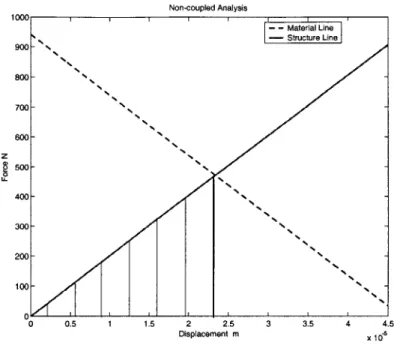
Non-coupled Analysis z 500
x
400- 300- 200-100 0 0 0.5 1 1.5 2 2.5 3 3.5 4 4.5 Displacement m X 10Figure 2-2: Material and Structure Loading Line for the Linear Systems
2.2
Linear and Non-linear Systems
The motivation for looking into non-linear systems comes from the diagram showing the inter-section of a material load line and a structure load line on a force-displacement diagram, shown in figure 2-2.
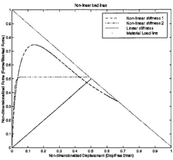
The area under the structure load line from the origin to the intersection is the actual mechanical work of the system. The area under the material load line is the total amount of energy available to do mechanical work. So if a structure load line, such as a curve, can encompass more area under the material load line before it intersect with the structure load line, it is possible that more mechanical work can be done on the structure. Thus, the actuation efficiency of the system will be increased. Such curves do exist and we can call them non-linear loading functions, while the corresponding systems called linear systems. Two sample non-linear loading functions are shown in Fig. 2-3. They are essentially the same functions defined
by Malinda for the purpose of comparison and discussion.
Linear loading function:
Flinear _ X (2.6)
Non-linear bad Ires
- - - Non-linear stiffness 1 0.9 - -- - - Nor-linear stiffness 2
Linear stiff ress 08 Material Load lIe
0.7 -0.6 -0. 90.4 .2 -.-0.1 0 0 on 0.1 0 0.2 0.3 0.4 0.5 0.5 0.7 0.8 09 1
2Nndinnnsbnalizd Dispbment (Disp)Fme Strain)
Figure 2-3: Comparison of Linear and Non-linear Functions
Non-linear loading function 1:
Fnon-lineari x
Fbi Xfree
.41 ex - . e 2
Non-linear loading function 2:
Fnon-linear2 1
Fbi 2
tanh
(66 Xf reex))2.3
General Analysis
The object we are going to study here is a piezo actuator. The linear constitutive equations of the piezoelectric are presented first, then the general actuator and sensor equations derived by Hagood et al [Hagood, 1990] are introduced. The work terms are derived using the actuator
and sensor equations and then applied to one dimensional linear and non-linear cases.
(2.7)
2.3.1
Linear Constitutive Equations
For small stresses and electric fields, piezoelectric materials follow a linear set of governing equa-tions which describe the electrical and mechanical interaction of the materials. The equation can be expressed as
(2.9)
D
d
e
TjEThese equations have four system states: T, the stress in six directions; E, the electric field in three directions; S, the strain in six directions; D, the electric displacement in three directions. The materials constitutive relation is a nine by nine matrix. This matrix can be reduced using either plain stress, plain strain assumptions, or by assuming one dimensional relations. Most of the work in this document will be using one dimensional relations, which is a two by two matrix.
2.3.2 Governing Equations for the coupled systems
The governing equations for the piezo active materials are the simplified actuator equation and sensor equation for quasi-static cases, which can be expressed as [Hagood, 1990]
KE -01 Xi
f
(2.10)
%_1"C V
Q1
Where K is the stiffness matrix for the active materials; 01 is the electromechanical cou-pling terms; CS is the capacitance of the active materials under constant strain and x1, V1, fi
and Q1 are the displacement, voltage, force and charge vector respectively. Dynamic terms are neglected since the tests were done quasistatically.
For the non-piezoelectric structure, force-displacement relation can be written as:
f,
= kox, (2.11)Where k, is the stiffness of the structure and can be either linear or non-linear with respect to x, the displacement of the structure.
2.3.3
Compatibility and Equilibrium
The states of the structure and active material are related by compatibility and equilibrium requirements.
Force equilibrium:
fi =
fs
(2.12)Compatibility:
X1 = -z8 = x (2.13)
From equation 2.10 we have
- =
fi
(2.14)Substitute equation 2.12 and equation 4.21, we have
k, = (2.15)
k8 + KE p1
This is an implicit relationship between V and x. which is automatically satisfied during the test. Therefore, this equation can be used to determine displacement of the active material when
a voltage is applied or for an expected displacement, the required voltage can be determined
by solving this equation iteratively.
2.3.4 Electrical Work
Electrical work is defined in equation 2.3. From equation 2.10:
Q1
=1P+1C
V1 (2.16)Substitute equation 2.15 into 4.18, we have
Q1 = 1V1 +T V +CS V (2.17)
Then the variation of Qi in terms of V1 can be expressed as
6Q1=
[ k, +K 9T91V1 dk, dx + CP 1 b 1 (k +K)2dx dV
Substitute equation 2.18 into equation 2.3, we have the electrical work expressed as
fVf [
ofo
1v
1
7
WE=+C
1 vk, + K P1 Og 17V12 dk, dx1
(ks +
KEj)2dxdV
12.3.5
Mechanical Work
Mechanical work is defined in equation 2.1, where
F = ksx
Finding the variation of x using equation 2.15, we have
1 k, + K (2.19) (2.20) (2.21) 01V1 dk dx (kP+K)2 dx dV
Substitute equation 2.20 and equation 2.21 into 2.1, we will have the mechanical work expressed as v kOT1V WM (ks
+
K) 2 1 V1dk, dx
1
k,
+ K
dx dVJ
1 (2.22)2.3.6
Actuation Efficiency
The actuation efficiency of the system is defined in equation 2.5, which is simply the ratio of equation 2.22 to equation 2.19.
2.4
One Dimensional Linear Systems
2.4.1
Expressions for Linear Systems
The systems discussed here has been shown in Fig. 2-1. For linear systems,
dk 8 0
dx (2.23)
And assume Vo = 0 and Vf = V1, equation 2.19 and equation 2.22 can be simplified and expressed as pT 1 WE= 12+ 1 k,6T61 WM= 12
2
(ks + C)2
(2.24) (2.25)2.4.2
Constitutive Equations
The central axis of the actuator and structure is regarded as the 3-direction of the systems. Linear material relations is used and constitutive equations 2.9 is simplified for one dimensional cases. The one dimensional constitutive equations in 3-direction can be written as
33 d33 d3 3 T 633 T3 E3 (2.26)
This equation can be rewritten to have strain as the free variable, then
T3 D3 J
[
E -e 3 3 S 633 S3 E3}
(2.27)From equation 2.26 and equation 2.27 we can find the following relations
1 33
e33 = d3 3cE3
(2.28)
E= - d 33
(2.30)
2.4.3
Finding the Constants in Work Expressions
To find the constants in the work expressions, i.e. equation 2.24 and equation 2.25, The Ritz method is used. Electrical and mechanical mode shapes , which satisfy the prescribed voltage boundary conditions and the geometric boundary conditions of this specific problem respectively are assumed as
IfE = X(2.31)
1
T = (2.32)
1p1
The assumed mode shapes can be used to find C, K Eand 01 using the equation developed by Hagood et al [Hagood, 1990] P1= JN TCENxdV1 (2.33) -
I
cE dVl cp1 01vpI
NfetNdV1
(2.34)
e33 +dV1 e33Api 1P1 P1 = JNesNvdVp1 (2.35) S i - e3 dVpl _ 3Api 1P1For a one dimensional linear structure, we have
A8
k - Cs
is
(2.36)
2.4.4
Simplified Expressions for Electrical and Mechanical Work
Assume that the structure and the piezoelectric have the same effective length and the same cross sectional area, then we have
As = Ap1 = A
is = 'pi =
1
(2.37)
(2.38) Substitute equation 2.33, 2.34, 2.35, 2.36, 2.37 and 2.38 into equation 2.24 and 2.25, we will be able to find the simplified expressions for mechanical work , electric work and actuation efficiency. Mechanical Work 1 A y ce 2M (2 c 33 s) VV-~Vi (c,33+ Cs)2 Electrical Work 1
AV
WE = -- V21l 2 633 +)3
(2.40) c3 + Cs)We can further simplify these two equations by taking advantage of the material coupling coefficient expressed as
(2.41) d 2
k 33
And the relation expressed in equations 2.28, 2.29 and 2.30. Then the mechanical work and electrical work will be
Mechanical Work
WM
1A2 3a
2
1
(1 + a)2(2.39)
Electrical Work WE 1633 2)3 Where a = S= (2.44) C33 kp
2.4.5
Actuation Efficiency
Actuation efficiency of the one dimensional linear system can be determined by equation 2.42 and 2.43, which is
k
2aWout - 33(1+a)2
(2.45)
Win 1 -
ck
3This expression is exactly the same as which derived by Giurgiutiu [Giurgiutiu, 1997] and Davis [Davis, 1999] respectively, but we use a different approach here.
It can be shown mathematically that equation 2.45 has a peak at
a = (2.46)
#1 -k3 And the maximum value is
k 2
(1Va= 33 2 (2.47)
2.4.6
Discussion on Actuation Efficiency
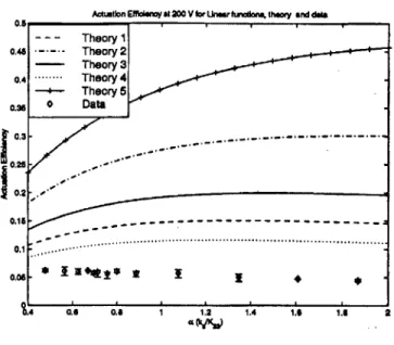
To better understand the expression we have derived here, actuation efficiency is plotted in Fig. 2-4 with the impedance matched system efficiency by Hall and Prechtl, equation 1.2, for comparison.
This figure shows that when material coupling coefficient is small, the actuation efficiency correlates the impedance matched systems efficiency. However, when material coupling coeffi-cient is significantly large, there is a big difference between the two due to higher electromechan-ical coupling. In addition, the peak value of the actuation efficiency occurs at a stiffness ratio larger than one, while the impedance matched system efficiency always occurs at the impedance matched condition.
Actuation Efficiency from coupled and uncoupled Analysis for linear systems S0.25 A) LL. 0.2- -C 0 K33=0.69 +- 0.15 -0.1 - K33=0.50 0.05 ----10-2 10 100 101 102
Stiffness ratio, alfa=Ks/K33E
Figure 2-4: Comparison of Actuation Efficiency of Linear Systems with Different k33 The relations of peak actuation efficiency and the corresponding stiffness ratio with the material coupling coefficient is illustrated in Fig.2-5.
2.5
One dimensional Non-linear Systems
2.5.1 General Analysis
In genaral, we can not find a close terms of V1, the applied voltage to equation 2.20 and equation 2.36 to the following form:
form solution for mechanical work and electrical work in test sample. For the convenience of analysis, we can use rewrite the non-linear functions, equation 2.7 and 2.8, in
fS = ksx = cocxA
(
is
Where co is a constant independent of x, and cx is the non-linear part of the stiffness. For nonlinear function 1:
cx = 41 exp-5.45(Xfree \ xNe / 22 (2.49) 2.48)
Actuation Efficiency and Stiffness Ratio Vs. K33 2.5 1.5 0" U, -0.2 0.3 0.4 0.5 0.6 0.7 0.8 0.9 1 materia coupting coefficienct k33
Figure 2-5: Max. Actuation Efficiency vs. k3 3 for 1D Linear Systems
For non-linear function 2:
cx = - (tanh (6 6 x))(2.50)
If we substitute equation 2.49, into equation 2.15, for example, we will have
= V(2.51)
C$1A541 exp (",,.. 2+K
It is obvious that there is no close form solution for x in terms of V1. Therefore, we can not
find close form solutions for mechanical work and electrical work for such non-linear systems by simply substituting equation 2.51 in to equation 2.19 and equation 2.22. To find a close form
solution, we need to express mechanical and electrical work in terms of the displacement of the
active materials.
2.5.2 Mechanical and electrical Work in terms of Displacement