The French biofuels mandates under cost uncertainty - an assesment based on robust optimization

HAL Id: hal-03206367

https://hal-ifp.archives-ouvertes.fr/hal-03206367

Preprint submitted on 23 Apr 2021

HAL is a multi-disciplinary open access

archive for the deposit and dissemination of sci-entific research documents, whether they are pub-lished or not. The documents may come from teaching and research institutions in France or abroad, or from public or private research centers.

L’archive ouverte pluridisciplinaire HAL, est destinée au dépôt et à la diffusion de documents scientifiques de niveau recherche, publiés ou non, émanant des établissements d’enseignement et de recherche français ou étrangers, des laboratoires publics ou privés.

The French biofuels mandates under cost uncertainty

-an assesment based on robust optimization

Daphné Lorne, Stéphane Tchung-Ming

To cite this version:

Daphné Lorne, Stéphane Tchung-Ming. The French biofuels mandates under cost uncertainty - an assesment based on robust optimization: Cahiers de l’Economie, Série Recherche, n° 87. 2012. �hal-03206367�

IFP Energies nouvelles - IFP School - Centre Économie et Gestion 228-232, av. Napoléon Bonaparte, F-92852 Rueil-Malmaison Cedex, FRANCE

!" #$%& #

Septembre 2012

Les cahiers de l'économie - n° 87

Série Recherche

[email protected]

La collection "Les cahiers de l’économie" a pour objectif de présenter des travaux réalisés à IFP Energies nouvelles et à IFP School, travaux de recherche ou notes de synthèse en économie, finance et gestion. La forme

peut être encore provisoire, afin de susciter des échanges de points de vue sur les sujets abordés. Les opinions émises dans les textes publiés dans cette collection doivent être considérées comme propres à leurs auteurs et

ne reflètent pas nécessairement le point de vue d’ IFP Energies nouvelles ou d' IFP School.

Pour toute information sur le contenu, prière de contacter directement l'auteur.

Pour toute information complémentaire, prière de contacter le Centre Économie et Gestion: Tél +33 1 47 52 72 27

The views expressed in this paper are those of the authors and do not imply endorsement by the IFP Energies Nouvelles or the IFP School. Neither these institutions nor the authors accept any liability for loss or

The French biofuels mandates under cost uncertainty – an assessment

based on robust optimization

ڏ

Draft paper

Daphné LORNE a Stéphane TCHUNG-MING b,*

Abstract

This paper investigates the impact of primary energy and technology cost uncertainty on the

achievement of renewable and especially biofuel policies – mandates and norms – in France

by 2030. A robust optimization technique that allows to deal with uncertainty sets of high

dimensionality is implemented in a TIMES-based long-term planning model of the French

energy transport and electricity sectors. The energy system costs and potential benefits

(GHG emissions abatements, diversification) of the French renewable mandates are assessed

within this framework. The results of this systemic analysis highlight how setting norms and

mandates allows to reduce the variability of CO2 emissions reductions and supply mix

diversification when the costs of technological progress and prices are uncertain. Beyond

that, we discuss the usefulness of robust optimization in complement of other techniques to

integrate uncertainty in large-scale energy models.

JEL classification: C61, Q42, Q48

Keywords: Biofuel policies; Energy vulnerability; Climate change; Robust optimization, uncertainty. __________________________________

ڏ

We are grateful to Alireza Tehrani, Amit Kanudia, Denise Van Regemorter, Andrea Diaz and Claire Nicolas for insightful comments and suggestions on this work. Any remaining errors are ours. Earlier versions of this work were presented at the 2012 MONDER Workshop, the Chaire Economie du Climat Seminar, and the 2012 International Energy Workshop.

a Economics and Environmental Evaluation Department, IFP Energies nouvelles, 1-4 avenue de Bois-Préau, 92852 Rueil-Malmaison, France. E-mail: [email protected].

b Economics and Environmental Evaluation Department, IFP Energies nouvelles, 1-4 avenue de Bois-Préau, 92852 Rueil-Malmaison, France. E-mail: [email protected] and CREDEN, Université de Montpellier 1, Avenue Raymond Dugrand, CS 79606, 34960 Montpellier Cedex 2, France.

1 INTRODUCTION

The global context of European energy policies is generally presented as grounded on three main objectives: competitiveness, security and sustainability. As a part of this global policies, mandates and norms were defined for the transport sector. The Renewable Energy Directive 2009/28/EC aims to promote the use of energy from renewable sources in the European Union. Among the main targets there are the 3x20 objectives on the European energy system: (i) 20% of renewables in the energy sector in 2020 (10% in transport); (ii) a reduction in EU greenhouse gas emissions of at least 20% below 1990 levels; (iii) gaining 20% in global energy efficiency. The RED required Member States to submit national renewable energy action plans by 2010 (Kautto and Peck, 2011). These plans provide detailed roadmaps of how each Member State expects to reach its legally binding 2020 target for the share of renewable energy in its final energy consumption (e.g., the French National Renewable Energy Action

Plan). Finally, the Fuel Quality Directive (2009/30/EC), introduces a mechanism to monitor and reduce greenhouse gas emissions from transport fuels. Notably, the article 7a mentions that the fuel suppliers are obliged to reduce their life-cycle GHG emissions per unit of energy from fuel and energy supplied by 6% by 2020, compared to 2010 level.

The need to decarbonize the transport sector has become a growing concern in a context of climate change, energy security and anticipated scarcity of fossil resources. In other terms, introducing biofuels in the transport energy mix is a potential source of double dividends because they allow to reduce the carbon footprint of transport1 and diversify energy supplies

1

The energy and agricultural effects of the EU biofuels targets (on their own, or as part of the more global Climate-energy package) have already led some attention. Kretschmer et al (2009) show in a CGE framework that the sole EU emissions targets do not trigger biofuel production (which might be explained by high marginal abatement costs of fuel and transport technologies compared to other sectors; see e.g. Smokers et al (2009)). Lonza et al. (2011) provide a detailed technical investigation of potential scenarios for transport to reach the renewable energy targets in 2020. In a broader scope, Labriet et al. (2011) analyze the implementation of the EU Renewable Directive in Spain, observing that compared to the actual situation, the main effort to reach the 2020 targets should rely on greening the transport and industry sectors.

simultaneously. From an environmental perspective, mandates and norms are recognized to provide means to reduce environmental damages, although not necessarily as efficient as taxes or markets2. The diversification issue is more rarely addressed3, and even more rarely quantified. Still, biofuels have been identified as an option to mitigate the various risks of energy dependence (Kher (2005); Russi (2007); Demirbas (2009)). These combined benefits are rarely assessed simultanesouly; Criqui and Mima (2012) propose a prospective view of such climate-diversification double dividends strategies.

However, the costs and benefits of imposing biofuels mandates and norms should be assessed in the light of the large uncertainties surrounding this pathways, in terms of availability and costs of biomass and biofuel technologies (Schade and Wieselthal, 2011). By extension, the potential costs and benefits of the biofuel mandates and quality norms should be assessed with respect to uncertain relative costs of biofuels compared to conventional fuels. Some of the rare examples of such approaches include Rosakis and Sourie (2005) and Schade and Wiesenthal (2011), who use Monte-Carlo simulation to highlight the large variations in biofuel subsidies depending on key macroeconomic variables. Energy systems involve (i) long-lasting, irreversible investments, some of which are today in R&D phase (ii) the use of

2

Recent work indicate that mixes of fossil (carbon) fuel taxes and biofuel subsidies can help stimulate the development of biofuels, as long as part of the revenues from taxes is recycled in the subsidies (Timilsina et al, 2011). Interestingly Lapan and Moschini (2011) complement this result by showing that integral recycling makes the price instrument equivalent to a quantity mandate.

3

Transport currently relies on fossil fuels for more than 95% of its energy supply; this fact puts the sector in a situation of "energy vulnerability". Percebois (2006) defines this concept as "a situation in which a country is not able to make voluntary energy policy choices, unless at an unbearable economic or political cost"3. Vulnerability with respect to a given resource is by nature an externality, because it generates "costs on the economy that [are] not reflected in the market price [of that resource] or in private decisions regarding the use [of that resource] instead of other alternatives" (Bohi and Toman, 1993). These effects shall be considered in the short run (e.g., through price volatility) or in the long run (e.g. through sustainable rises in energy prices that affect the energy system and the economy as a whole). Energy vulnerability has emerged as a great concerned in the 1970s because of the oil shocks (Ward and Shively (1981); Kline and Weyant (1983)). As defined by Yergin (1988), the objective of energy security should then be to "assure adequate, reliable supplies of energy at reasonable prices". While both supply and demand side measures are likely to solve par of the issue (Andrews, 2005), diversification of energy supplies have long been identified as a mitigation option (Stirling (1994); Nakawiro and Bhattacharyya (2007); Nakawiro et al (2008); Gnansounou and Dong (2010); Cohen et al (2011)). Although of

very volatile primary energy sources (crude oil, natural gas, coal, biomass, etc.), so that decisions concerning biofuel policies must be taken now for the next decades. Decisions must be taken in the presence of global uncertainty, and biofuel policies do not escape this remark. Practically, long-term assessments of biofuel policies should account not only for their costs, but also for their potential multiple benefits, and in a context of pervasive uncertainty that embrace both microeconomic (technology costs) and macroeconomic (energy prices) variables.

This work is grounded on this last observation; its contributions are twofold. From a methodological perspective, we argue that robust optimization techniques are appropriate for introducing cost uncertainty (primary energy sources, technology investment) from many sources in long-term energy models. Similar methods were recently introduced in large-scale prospective models (Babonneau et al, 2012) for different purposes. We explain that in the process of addressing various levels of uncertainty à la Bertsimas and Sim (2004), we "endogenously" generate various relative cost systems that determine the competitiveness of the various pathways included in the model. Those cost scenarios are generated according to a worst-case logic, and is consistent with a specific definition of risk preferences.

This method captures the effect on decisions of numerous uncertainty sources, what stochastic optimization more hardly does. On the other hand, it endogenously accounts for uncertainty, while Monte-Carlo "only" performs advanced sensitivity analysis. Moreover, because it relies on set-based uncertainty models, it avoids the recourse to (often ad hoc) definition of probability densities of uncertain parameters. In short, we propose to test how a robust optimization technique can be used to evaluate a public policy in a system model, accounting for such systemic uncertainty.

much more general nature, these issues naturally arise in the transport sector (isolated from the rest of the energy system).

We apply this methodology to an appraisal of the French biofuel policies, including the RED, the NREAP and the FQD. Under various uncertainty levels for economic parameters included in the model, we evaluate the technical and hedging extra-costs of the biofuel mandates and norms with respect to a no-policy case. We then highlight the multiple benefits offered by this policies, in terms of CO2 emissions and system diversification. Accounting for uncertainty

also allows to reduce the variability of CO2 emissions reductions and supply mix

diversification when the costs of technological progress and prices are uncertain. This highlights another potential benefit for implementing biofuel mandates in the presence of uncertainty – a hedging one.

The paper is structured as follows. In section 2, we present the long-term MIRET model for the French energy-transport system. Section 3 then presents the robust optimization technique implemented and insists on some theoretical implications. In section 4, we describe the scenarios constructed for this study and results on the appraisal of the French biofuel policies. Section 5 concludes on some methodological and policy insights.

2 AN ENERGY-TRANSPORT SYSTEM MODEL

In this section, we present the IFPEN-developed MIRET model: a long-term, multi-period, techno-economic planning model that covers the energy-transport system in detail. Its scope is continental France, and the time horizon is 2030, with 2007 as base-year.

The TIMES model generator is used as a modeling framework. Under this well established paradigm (cite references for history and recent uses), a Reference Energy System is built to cover the stock of equipment and flows for the reference year, the characteristics of future technologies, the potential and costs for primary energy. This being given, the model aims at

providing final energy services / energy (mobility for passengers and freight, electricity, etc.) at minimum cost. To do this, investment and operation decisions are made for the technologies embraced in the model ; subsequent primary energy uses are obtained.

2.1 General presentation

The model schematics is presented in Figure 1. It presents a block diagram that links elements described in the model according to four main dimensions: energy supply, technologies, demand and policies (Loulou et al, 2005).

Figure 1: model schematics

The reference energy system is thus composed (from left to right) of:

- a primary energy supply block: includes imported fossil energy (crude oil, coal, natural gas), biomass (starch crops – wheat, corn; sugar crops – sugar beet; oil crops – rapeseed, sunflower ; lignocellulosic biomass – forest wood, crop residues, dedicated energy crops), imports ;

- an energy technology block, whose technologies transform primary energy into energy vectors and energy services: it includes oil refining with a detailed process-based model derived from IFPEN OURSE model4 (including 20 process units and products specifications, see Saint-Antonin (1998) or Tehrani (2008) for detailed presentations), biofuel units (first generation – ethanol, FAME5, HVO6; second generation – ethanol and synthetic FT-Diesel), electricity generation (power plants – all technologies; combined heat and power), preparation of fuels for transport at blending (diesel, biodiesel B30, gasoline grades E5 and E10 and E85, jet fuel – including fossil and bio bases), and end-use technologies for road mobility (personal vehicles and Light – thermal, hybrid, plug-in hybrid / gasoline, diesel, natural gas, flexfuel, electric cars; buses and trucks – thermal, hybrid / gasoline, diesel, biodiesel);

- a final energy / energy services demands block: Electricity demand by time period (four days representing each season, the power load being hourly described for each of these days), mobility demands (short and long distance for passenger vehicles and buses, traffic for LUV, demand for freight mobility), demands for exported products (oil products, electricity);

- a policies block: includes measures and constraints of several types affecting all sectors. Some are of microscopic nature, such as quality norms for refinery products, number of functioning hours of fuel turbines power plants, etc. Some are macroscopic in nature, e.g. sectoral carbon tax. Three measures aiming to develop biofuels will be detailed below: the National Renewable Energy Action Plan (NREAP) for France, and the enforcement of two European Directives (RED and FQD).

2.2 Basic formalism

4

Some process units were removed from the initial model, and the quality of the crude supply was fixed to an average "typical crude cocktail".

5

FAME: Fatty Acid Methyl Ester 6

The objective function of the underlying linear program takes the form:

( )

( )

( )

( )

( )

( )

( )

( )

t periods

INVCOST t INVTAXSUB t INVDECOM t

OBJ DISC t FIXCOST t FIXTAXSUB t VARCOST t SALVAGE LATEREVENUES t

∈

+ +

= + + + −

−

It is simply the discounted sum of investment costs (including taxes and subsidies), decommissioning costs, fix costs (including taxes and subsidies) variable costs, and economic value of investments whose life extends beyond the time horizon. Because the energy model used here relies on the principle of intertemporal optimization with perfect foresight (Loulou et al, 2005), it can be stated in the standard form of a single linear program and solved like a static one (Dantzig, 1959). The objective function and constraints then encompass the intertemporal relationships between variables at different dates (e.g., the stock of equipment at time t is the sum of new investments in t , plus all investments realized for all

τ

<t, minus all decommissioning occurred until t ).

The two linear programs

( )

P_ref and

(

P_bio

)

refer respectively to the "reference" case and the "biofuel policies" case:

(

)

( )

( )

( )

( )

( )

min . . 0 0 T ref c x s c Ax b y Tx P Kx k Qx q Sx s x

τ

λ

ω

σ

≥ = ≤ ≤ ≤ ≥

(

)

( )

( )

( )

( )

( )

( )

( )

( )

≥ ≤ ≥ ≥ ≤ ≤ ≤ = ≥ 0 0 0 . . min x f Fx Rx n Nx s Sx q Qx k Kx Tx y b Ax c s x c P T bio

φ

ρ

η

σ

ω

λ

τ

c is the column vector of all discounted unit costs. The equations Ax≥ correspond to the b

final demands of energy and energy services to be satisfied. The equation set Tx=0 describes the fundamental input-output relationships of each technology, namely the mass or energy

balance of each technology. The set Kx≤k includes all capacity constraints, either technology or resource based. For example, (i) the electricity produced by a given technology

is limited by the combination of the stock installed and seasonal or hourly availability factors,

(ii) the use of scarce resources, e.g. woody biomass, are limited for use for power, heat,

combined heat and power and biofuels production. Qx≤ accounts for the quality equations q

of some of the products. This is especially the case of refinery products, whose quality must

respect certain specifications to be marketed7. Finally, the set Sx≤ includes all sorts of s

institutional constraints (e.g., the French legislation limits the number of functioning hours of

certain power plants – notably fuel turbines), calibration constraints and share constraints.

The program P includes three additional sets of constraints. The transport declination of the _bio

RED, Rx≥ , describes the obligation to incorporate at least 10% (LHV) of renewable energy 0 in transport beyond 2020. It is formulated as follows:

1 1 2 2 2 2.5 Re 10% G G G G nelc AllTransports Terrestrial Transports LHV Q LHV Q Q EnergyConsumed × + × + ≥

There, it is worth mentioning that second generation pathways double-counted (i.e., 1MJ of

second generation biofuel counts for 2MJ), and that renewable electricity is counted 2.5 times.

Moreover, the total energy consumed does not account for the energy consumption of air

transportation. This clearly tends to advantage the development of second generation biofuel

pathways and the introduction of biofuels as substitutes for jetfuel.

The French NREAP describes, for each renewable energy pathway (biofuels, electricity and

heat), the quantitative mandate to be achieved between 2012 and 2020; values are maintained

constant beyond that date.

7

Main specifications include (Tehrani, 2008) specific gravity and sulfur content (gasoline and diesel), vapor pressure, octane index, aromatics and olefins contents (gasoline), cetane index (diesel) or viscosity (fuel oil). Under a linear programming framework, it is assumed that the qualities blend in mass or volume. Otherwise, constraints are written as index (Babusiaux, 1990).

Finally, the FQD Fx≤ f , specifies that the emissions of each liquid fuel pool must reach a given level of reduction with respect to the fossil reference after 2020:

Re 0.96 Base Base AllBases InAFuel Fossil f Base AllBases InAFuel Q E E Q ≤ .

3 UNCERTAIN COSTS AND ROBUSTNESS

Robust optimization (RO) has been developed in mathematical programming since the 1970's.

Rather than relying on probabilistic models of uncertainties, RO is based on deterministic and

set-based uncertainty models. That is, "instead of seeking to immunize the solution in some

probabilistic sense to stochastic uncertainty, here the decision-maker constructs a solution that is optimal for any realization of the uncertainty in a given set" (Bertsimas et al, 2007).

Soyster (1973) was one of the first to use RO, considering data uncertainty in linear programs.

Assuming unknown but symmetric distributions for uncertain parameters, he defines the

robust counterpart of the nominal program as the solution to the worst-case deviation. This

approach guarantees the feasibility of the solution for any realization of the uncertain

parameters; however, it is very conservative. Other RO approaches have been developed since

then8. Robust optimization is rarely employed in the field of energy-economy modeling;

Babonneau et al. (2011) and Babonneau et al. (2012) propose some of the rare examples of

implementing robust control strategies. They analyze the effect of primary energy disruption

along risky routes or the effect of uncertainty on the level of availability of some

technologies. In the sequel of this section, we present a RO method which is capable of

capturing many uncertainty sources simultaneously; this allows to introduce "systemic"

3.1 The Bertsimas and Sim (2004) RO approach of linear programming – static case

Bertsimas & Sim's (2004) method of robust linear programming was chosen for this work. It

is adapted to deal with large uncertainty sets without loosing linearity nor dramatically

worsening the computational complexity (Gabrel and Murat (2008)). Let

( )

P be a linear program defined as:

( )

min , , 0 T n m n c x P Ax b x A x × ≥ ∈ ∈ ≥ .

Assume now that the cost coefficients of

( )

P are uncertain9 ; they can vary in a symmetric range c=

[

c−c cˆ, +cˆ

]

around the nominal value c ; no specific distribution is assumed. Bertsimas and Sim (2004) generalize Soyster's approach by noticing that it is unlikely that all

parameters will adversely deviate at the same time. More generally, it consists in controlling

the degree of "pessimism" on the cost coefficients of the objective function. Let then J ⊆ n

the subset of potentially deviating cost coefficients, andz_i∈ −

[

1,1 ,

]

∀ ∈i J a set of variables such that c_i =c_i+z c_{i i}ˆ ,∀ ∈ . Formally, the uncertainty set ϒ is symmetrical and polyhedral, i J

{

c_i z c z_{i i}ˆ _i 1, i J

}

ϒ = + ≤ ∀ ∈ . The idea is to control the number Γ ≤₀ J , representing the

maximal number of costs that may deviate; Γ is called the uncertainty budget. In the rest of ₀

8

See Ben-Tal et al (2009) for a deeper presentation. 9

Remark that the method is general enough to address uncertainty for any parameter of the problem, if it is formulated as follows:

( )

min 0, , 0, 0, , 1 m A b T c m m m z Ax bO A U b U z c x c U x O eye x x − ≥ ∈ ∈ − ≥ ∈ ≥ = =

this work, the deviations are constructed as ad-hoc fractions of the nominal values, ˆc_J =

α

c_J.

We then define an uncertainty scenario as a pair

(

Γ₀,α

)

,Γ ∈₀ 0, J ,α∈

[ ]

0,1 .

If xf is a feasible solution to

( )

P , the maximum deviation at xf for the protection level Γ ₀ is the solution of the linear program

( )

( )

( )

0 ˆ max 1 0 T f T J z Cx e z D z z

ϕ

µ

≤ Γ ≤ ≥

where Cˆ =diag c

( )

ˆ and e_J is a vector of ones. In short,

( )

D identifies the sets of Γ costs ₀ among n that – if reaching their maximal value – produce the maximum deviation. This

yields a nonlinear formulation; using strong duality, Bertsimas and Sim (2004) obtain an

elegant linear formulation of the robust problem,

( )

( )

( )

0 min ˆ 0, 0, 0 T T J J c x e Ax b y R e Cx z x

ϕ

µ

ϕ

µ

ϕ

µ

+ Γ + ≥ + ≥ ≥ ≥ ≥

In

( )

R , the system modeled is optimized for both the standard decision variables and the identification of the most sensible coefficients of the objective function.

3.2 Economic interpretation

The economic interpretation of the robust problem formulated above comprises at least three

components.

Firstly, the extra system cost due to robustness can be measured (for a given value of Γ and ₀ a maximum deviation of

α

) as the difference between the two objective functions,

(

* *

)

* * 0 T rob rob Hedging Technical substitutions c x x

ϕ

e

µ

∆ = − + Γ +

The global expression may be interpreted as a risk premium associated to the robustness level

(

Γ0,

α

)

. The first bracketed term represents the technical substitution cost due to uncertainty.

It is due to the fact that accounting for potential cost increases will induce technological

substitutions in the energy system that act as hedging strategies against cost increases of the

most sensible technologies. The second bracketed term consists in a pure financial cost, in the

sense that it comes straightforwardly from the use of technologies that will be used although

their cost may increase (in other words, the less substitutable technologies).

Second, we shall observe that varying the uncertainty budget actually corresponds to

endogenously varying the costs coefficients of the objective function. Using the primal form of

the deviation sub-problem, we get the following expression for the objective function at

optimum:

* *T _ˆ * *

J J J J J

Risk adjustment

Obj = c + z C x +c x

This means that at optimum, the relative costs come as a solution of the problem. The terms

(

*

)

ˆ

J J

c +z c correspond to risk-adjusted costs according to a worst-case logic. The dual version of this observation is equally meaningful; the shadow prices of the constraints are

now related by

ˆT T ₀

c+C z−A y≤ ,

which means that the shadow prices of the commodities are likewise risk-adjusted for the pair

(

Γ0,

α

)

. This has an important implication: in the process of varying the uncertainty budget,

assessment (defined by the deviation subproblem). This interpretation gives a sense, as

proposed in the sequel of the paper, to performing a systematic sensitivity analysis on the

uncertainty budget Γ , because it allows to test the model response to various cost regimes₀ 10.

Finally, when it comes to uncertainty, one naturally expects to find some connections with

risk preferences. There exists a relationship between robust linear programs and risk-averse

optimization; the link relies on the analysis of the uncertainty sets of the robust programs with

respect to specific families of risk measures (Bertsimas and Brown (2009); Natarajan et al

(2009)). Formally, the robust program

( )

R defined above is equivalent to the risk-averse problem

(

)

(

)

min 0 0 T r a r a z z c x P Ax b x

ρ

₋ − − ≤ ≥ ≥ where

ρ

r a−

( )

. is a coherent risk measure

11

(Artzner et al, 1999), generated by a combination

of Conditional-Value-at-Risk measures12 (Bertsimas and Brown, 2009). Consequently, the

robust version of the energy model used in this work will show a taste for diversity.

10

Other approaches, e.g. Bertsimas and Sim (2004), address the determination of an optimal uncertainty budget.

11

Artzner et al (1999) define a coherent risk measure

ρ

( )

. as satisfying the four following axioms:

- monotonicity: ∀

(

X Y,

)

∈ 2,X ≤Y

ρ

( )

X ≤

ρ

( )

Y . Intuition: ≤ defines statewise dominance (X ≥Y ⇔ ∀ ∈ Ω

ω

,X

( )

ω

≥Y

( )

ω

). Monotonicity means that if X performs better than Y for any realization of the uncertain parameters, then X cannot perform worse than Y in terms of risk.

- translation invariance: ∀

(

X t,

)

∈ × ,

ρ

(

X +t

)

=

ρ

( )

X −t. Intuition: if the cost is increased

3.3 Integration in an intertemporal framework

The energy model used in this paper relies on intertemporal optimization under perfect

foresight. Therefore, the two following principles should be used to formulate the problem

(Bertsimas and Thiele, 2006):

- uncertainty should propagate over time: deviated parameters in t will be deviated in

each subsequent period, for at least the same amount;

- consequently, there should be one uncertainty budget per period.

Let then t0be the first period at which parameters become uncertain ; let Jτ,∀ ≥ the set of

τ

t0

uncertain parameters for any subsequent period. According to the first principle, we should

have J_τ ⊆J_τ+1,∀ ≥

τ

t₀. According to the second principle, the maximum uncertainty budget

in any period should be max _t

t

J

τ τ ≤

Γ = . We get the formulation finally integrated in the model:

0 0 , , 0 min ˆ , , , 0, 0, 0 T T t t j j c x Ax b c x t j J x τ τ τ δ τ δ τ δ δ τ τ λ µ λ µ τ δ τ λ µ = = + Γ + ≥ + ≥ ∀ ≥ ∀ ≤ ∀ ∈ ≥ ≥ ≥

This formulation clearly shows the consequence of propagating uncertainty over time: more

weight is given to early period, which implies that early diversification is to be expected.

- subadditivity: ∀

(

X Y,

)

∈ 2,

ρ

(

X +Y

)

≤

ρ

( )

X +

ρ

( )

Y . Intuition: adding up the costs of two

system can not increase risk with respect to their separate risk exposures.

positive homogeneity: ∀

(

X,

α

)

∈ × ₊,

ρ α

(

X

)

=

αρ

( )

X . Intuition: similar positions positively add

up.

12

The CVaR is defined as the expected value of losses beyond the Value-at-Risk of a given position . The VaR itself is the value of losses that can be guaranteed at a given level, e.g. 95%. See Natarajan et al (2009) for a proof in the case of a discrete uniform distribution, and Bertsimas and Brown (2009) in the general case.

4 ASSESSING THE FRENCH BIOFUEL POLICIES UNDER UNCERTAINTY

In this section, we apply the methodology explained in the two previous sections to analyze

the rationales of the French biofuel mandates, and provide both policy insights and

methodological remarks.

4.1 Scenarios

The scenarios implemented to run the model include four main components: primary energy

supply, technologies, demands and policies.

Table 1 provides a list of the main sources used to elaborate the scenarios. Some of these

assumptions are detailed in appendix.

Scenario

components Sector

Data sources Fossil energy IEA (2011) Agricultural biomass INRA

Woody biomass FCBA

Refining Internal IFPEN Biofuels Internal

IFPEN Road mobility (Passengers

and Freight) Internal IFPEN Power plants EDF, IEA (2010), MINEFI (2008) Other oil products IFPEN/LEPII Pass. And Freight mobility CAS (2009) Electricity RTE (2011) Carbon price IEA (2011) Biofuels EC (2009), EC (2010) Primary energy Energy technologies Demand scenarios Policies

Table 1: sources for numerical assumptions

Two clear-cut atmospheres are described. In the Reference Scenario (Ref), no renewable

energy production target is enforced. However, the actual promotion mechanisms (subsidies

to investments in new technologies or feed-in tariffs) for the integration of renewable

Policy Scenario. It covers the perimeter of ETS-eligible installations, which excludes the

transport sector (no carbon tax system in the transport sector). Existing norms of energy

efficiency applying to end-use technologies are implemented. In the Biofuel Policies Scenario

(Pol), The French NREAP objectives are enforced for the period 2010-2020, and maintained

for the period 2020-2030 at their 2020 value. The RED is enforced beyond 2020 to ensure a

lower rate of integration of renewable fuels in the transport sector (10%). Finally, the Fuel

Quality Directive limits the carbon footprint of fuel production pathways. Otherwise, all other

numerical assumptions are the same as in the Ref scenario. The three policies are evaluated at

the same, as a renewable energy policies pack.

One important policy element regarding fuels for transport is the tax regime. In both Ref and

Pol scenarios, taxes and incentives are kept at their current levels. This includes the domestic

tax on petroleum products for fossil fuels, tax exemptions and subsidies for ethanol, biodiesel

and E85 fuels.

The uncertainty model We assume that investment costs of new technologies available from

2015 and beyond are not known with certainty. For each of these technologies, the uncertainty

model follows that described in section 3.1 (α =0.1 and α =0.2 are chosen for sensitivity analysis). On top of that, it is assumed that the unit costs of primary energy are also subject to

uncertainty. This concerns fossil primary energy (crude, natural gas and coal), biomass

(agricultural crops, imported vegetable oils, dedicated energy crops and agricultural and forest

residues), and final energy imported (electricity, ethanol). And at last, the price of CO2 is also

considered in the uncertainty set, as a part of the WEO NPS price scenario13. These

assumptions are summarized in Table 2.

13

Not all cost coefficients of technologies are considered in the uncertainty set. Non-energy variable costs and taxes are left aside. However, investments and energy costs cover roughly 80% of the total system cost.

Scenario

components Sector

Uncertainty source

Fossil energy Price Agricultural biomass Price Woody biomass Price

Refining None

Biofuels Investment cost Road mobility (Passengers

and Freight)

Investment cost Power plants Investment

cost

Policies Carbon price Price

None Primary energy Energy technologies Demand scenarios

Table 2 : parameters affected by uncertainty

The overall uncertainty set comprises 91 cost parameters. Under the dynamic uncertainty

model chosen, this makes a total of ~900 constraints to be added to the original model14. In

sequel, the uncertainty budgets at each period are varied proportionally: if

( )

0

t t t≥

Γ = Γ is the vector of uncertainty budgets over time, then we vary h∈

[ ]

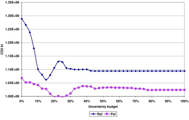
0,1 such that Γ = Γ . _h h

4.2 Global outlook – total system cost

We obtained from the set of optimizations performed the optimal total system cost,

decomposed as the sum of technical and hedging costs, in the Ref and Pol scenarios. Figure 2

presents the relative energy cost REC₍Scen_Γ,α),Scen∈

{

Re ,f Pol

}

and total cost

( , ),

{

Re ,

}

Scen

RTC_Γα Scen∈ f Pol of each scenario relative to the Ref case with no uncertainty:

( ) ( ) ( ) ( ) ( ) ( ) , , Re 0, 0.1 , , Re 0, 0.1 , Scen Scen f Scen Scen f EC REC EC TC RTC EC α α α α α α Γ Γ Γ= = Γ Γ Γ= = = = 14

1 1.05 1.1 1.15 1.2 1.25 1.3 0.0% 10.0% 20.0% 30.0% 40.0% 50.0% 60.0% 70.0% 80.0% 90.0% 100.0% Uncertainty budget R E C , R T C

Ref Technical Cost Ref Total Cost Pol Technical Cost Pol Total Cost

Figure 2: Total system cost

Increasing the uncertainty budget naturally raises the total system cost under any policy

regime. Between no hedge (h= ) and full hedge (0 h= ), the total cost raises by ~10% for 1

Ref and ~12% for Pol. Setting renewable and biofuels policies clearly induce higher technical

system costs. In any case, the implementation of the renewable policies has an additional

system cost increasing from 12% and up to 13% more, depending on the level of uncertainty.

Implementing these policies also exposes the system to greater hedging costs: hedging

represents up to 20% more in the cost decomposition of the objective function in the Pol

scenario.

The shape of the total cost envelope appears to be concave15. More remarkably, the cost

decomposition in energy system and hedging costs conserves this property for each of the cost

15

A standard result of linear programming states that when minimizing cost, the parametric analysis of a linear program based on a cost coefficient yields a concave locus of optimal objectives (Maurin, 1963).

component16. Loosely speaking, the least-cost optimization without uncertainty offers some

unused (because non-economical) technological substitution options. The standard result of

linear programming is that it provides a merit-order based upward sloped supply curve for

each of the good consumed in the model; risk adjustments on costs modify this merit order.

Some of the unused option economical when costs are adjusted; but, this potential is limited.

Consequently, the stock of substitution options become more "scarce" as the uncertainty

budget grows and more costs are risk-adjusted – progressively going back to the initial

relative costs system.

Hedging costs vary likewise with the uncertainty budget. This situation reflects two

phenomena. First, the substitution options may be limited or inexistent for some pathways. In

that case, there is no choice but to support the extra cost associated to adverse cost deviations.

Second, it may be efficient to support this extra-cost because some technologies have existing

stocks; switching to other technologies or pathways would induce high opportunity costs.

Assume for example an adverse increase of crude oil price; it offers a good illustration of the

two: oil cannot be fully substituted for the production of naphta (an input for petrochemicals)

and is almost the only single energy supply in the transport sector. The fact that its price raises

by 10 or 20% does not make the use of the existing vehicles stock irrelevant with respect to

anticipating the fleet renewal.

Finally, one shall notice that both energy system and total cost become almost flat beyond a

certain uncertainty budget (between 30% and 40%). This means that beyond a certain

threshold, the hedging cost defined by all processes whose constraints are active at optimum

do not change; all arbitrage opportunities are gone. In this region, all changes in absolute costs

do not change relative costs anymore.

16

There is no general theorem in linear programming that states the curvature of subfunctions of the objective when one coefficient varies.

4.3 Global outlook – the CO2 – diversification nexus

On the other hand, one shall quantify the potential gains brought by the implementation of

renewable mandate and norms. Figure 3 shows a global warming indicator in the form of

cumulated CO2 emissions over 2010-2030, GW_(ΓScen_,α) as a function of the uncertainty budget.

A diversification index was built as on the basis of costs as an average Herfindhal-Hirschman

index over 2010-2030. If there are M economic activities (energy import, energy

transformation and/or transport, energy use in final devices etc.), the market share at t of any

process i∈ 1,M is 1, i i t t j t j M c c

σ

∈ =

. All costs (investment annuities, energy supply, fix and

variable costs) are taken into account. Then

( )

2 1, 10000 i t t i M HHI σ ∈ = , and ( , ) ( , ), 0 0 1 Scen Scen t t t T HHI HHI T t α α Γ Γ ≤ ≤ =

− . Figure 4 plots the average HHI over process market shares17, for the period 2010-2030, always with respect to the uncertainty budget.

17

Most technologies/processes included in the model are affected by uncertainty. Comparing shares thus only makes sense on a cost basis, because production levels and installed capacities have different units. In short, diversity needs to be addressed in a systemic way, because uncertainty is addressed that way.

1.00E+06 1.05E+06 1.10E+06 1.15E+06 1.20E+06 1.25E+06 1.30E+06 1.35E+06 0% 10% 20% 30% 40% 50% 60% 70% 80% 90% 100% Uncertainty budget C O 2 k t Ref Pol

Figure 3: Cumulated CO2 emissions

600 700 800 900 1000 1100 1200 1300 1400 1500 0% 10% 20% 30% 40% 50% 60% 70% 80% 90% 100% Uncertainty budget H H I Ref Pol

The implementation of renewable policies offers benefits in terms of CO2 emissions (up to

-17%) and energy supply diversification (up to -25%); this is consistent with the existing

literature on the subject. Interestingly, this result is robust to uncertainty: whatever the cost

scenario considered, the Pol scenario outperforms the Ref one on both criteria.

Second, cost variations for small uncertainty budgets (that is, the most unfavorable increases

of cost coefficients, h≤~ 20%) trigger technological hedging strategies that induce both reductions in CO2 emissions and diversification. In short, new technologies become

competitive, which allows to combine the two benefits. As will be detailed below, biofuels are

part of this strategy. It is there interesting to notice that uncertainty can be a driver that yields

the combination of both benefits, with orders of magnitude comparable to the implementation

of renewable policies: for h~ 10%, emissions and concentration indices are almost

comparables in Ref and Pol.

Increasing the uncertainty budget further (h≥~ 20%) shows a rebound, due to further changes in relative costs: the alternative technologies or resources are themselves subject to

risk adjustments.

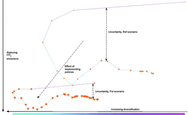
One striking observation out of Figure 3 and Figure 4 is that the variations of the indicators

induced by the variation on the level of uncertainty are reduced in the Pol scenario. To

confirm this, Figure 5 plots the locus of equilibrium HHI/CO2 points for all hedging levels.

That is, for both Ref and Pol scenarios, the

(

HHI₍Scen_Γ,α),GW₍Scen_Γ,α)

)

couples are plotted. On the figure, the size of each point is proportional to its relative total cost ₍Scen_{, )}

RTC_Γα , while the links

Figure 5: the locus of HHI/CO2 points, Ref and Pol

The effect of uncertainty on the diversity and climate change measures is ambiguous: changes

in the energy and technology costs may improve/worsen either indicator, or even both. This

ambiguity is inherent to the existence of pervasive uncertainty in any prospective study: the

relative competitiveness of energy sources and technologies are uncertain.

This appears clearly in Figure 5, where the CO2(HHI) curves are not monotonic. The "spread"

of each of the two curves on the plane reflects the dispersion of potential outcomes, due to

uncertainty on cost parameters. It is much smaller in the Pol scenario than in the Ref scenario.

Moreover, the Pol curve is translated to the lower left corner, indicating increased average

performances over Ref.

Overall, these results seem to indicate that although implementing renewable mandates and

diversification and (ii) reducing the field of possible outcomes on these criteria, in a context

of systemic uncertainty. This is of importance for policy analysis. If uncertainty could be

managed at the individual level just like the planner modeled in this study would, then

accounting for it would induce multiple benefits. But this is not the case; rather, uncertainty at

the investor level would probably limit investments. In such conditions, the cost induced by

the implementation of simple policies such as mandates and norms also covers some hedging

considerations that ensure a minimal improvement for the criteria considered.

4.4 The underlying biofuel technology choices

Beyond the macroscopic perspective presented in sections 4.2 and 4.3, one may question the

declination of these observations at the technology level. This is of interest for both (i) policy

makers, who practically often recourse to specific policies (mandates, taxes, subsidies) for

different technologies and pathways and (ii) technology experts and industrials who question

the relevance and risk of investing in the development of some of these technologies.

Figure 6 shows the cumulated 2010-2030 incorporation rate of biofuels in all liquid fuels, as a

function of the uncertainty budget. Naturally, biofuels are more widely incorporated in the Pol

scenario because of the enforced policy constraints. Remarkably, in this scenario, the lower

bound of incorporation only reaches 9% in physical terms. This echoes the results of some

existing studies, underlining the difficulty of reaching 10% of physical incorporation under

the existing policy designs (JRC, 2011). However, uncertainty can naturally trigger the use of

biofuels, as highlighted in the left part of the graph: for low values of h , the use of biofuels

increases due to changes in generalized relative costs. The effect is stronger in the Ref

0% 1% 2% 3% 4% 5% 6% 7% 8% 9% 10% 0% 10% 20% 30% 40% 50% 60% 70% 80% 90% 100% Uncertainty budget M a s s i n c o rp o ra ti o n r a te ( % ) Ref Pol

Figure 6: Biofuels incorporation rates

Then, Figure 7 shows the boxplot18 of the cost-based market share of each biofuel technology,

across all uncertainty scenarios, in the Ref case (left) and the Pol case (right). This allows to

measure the potentials and risks attached to each technology for various cost scenarios and

policy regimes.

Under the assumptions made, the recourse to 1st generation pathways (ethanol, FAME) shows

no-to-little variations, because of resource availability constraints. This is true irrespective of

the policy scenario considered. HVO pathways offer some potential for the period 2015-2030,

although rather "volatile". In 2020 and after, second generation biofuels – and especially BtL

– do never emerge in the Ref case, and rarely in the Pol case (mostly as outlying points). This

is due to either (i) the pessimistic nominal cost trajectories of these technologies, or (ii) the

technical characteristics of the technologies – efficiencies, or even (iii) the relative failure of

policies in place at this time horizon19.

In any case, second generation technologies seem rather "risky". This reflects the essential

message that biofuel technologies are nowadays not completely competitive. Their

market-driven penetration would require large adverse costs increases of competing fuels, more

drastic R&D efforts to pull costs down, which could be sustained by more ambitious public

policies (IEA, 2012).

5 CONCLUSION

18

The box plot summarizes for the populations (i.e., the 2010-2030 average market share for each technology and each uncertainty scenario), the following statistics: minimal value of the sample, 1st to 3rd quartiles, maximal value. Outliers are also represented.

19

Another explanation is linked to the earlier availability of HVO with respect to second generation technologies. Because the uncertainty model is built to that cost deviations are carried over across the whole horizon, the decision maker has a tendency towards early diversification; HVO allows to hedge early on, because it is mature earlier.

The analysis undertaken in this work aims at measuring the extra energy system cost

associated to the implementation of renewable and biofuel policies in France by 2030.

Compared to other existing research, we account for uncertainty of future costs of both

technologies and primary energy. For this purpose, a simple energy system model describing

the French transport and electricity sectors was augmented with a recent robust optimization

technique.

Under this framework, the system cost of the renewable/biofuel policies is augmented

between 10% and 20%, depending on the degree of uncertainty considered. However, the

potential benefits of such climate policies include the reduction of CO2 emissions and the

diversification of pathways for the supply of final energy service demands. These two benefits

correspond to a so-called double dividend. Moreover, we highlight that under cost uncertainty

and no major modification of tax regimes, the implementation of renewable energy mandates

allows to narrow down the performance of the energy system for CO2 emissions and supply

diversification. In that sense, climate policy mandates act as a hedge against adverse cost

increases of the major energy system costs. This suggests a third potential dividend for these

policies, that should contribute to balance their higher technical cost of implementation.

Moreover, uncertainty alone can be a sufficient driver to trigger the use of renewables (as

hedges), so that the mandates may be understood as a way of decentralizing the effect of

uncertainty about future costs at the agent level. These findings are of interest from a policy

perspective, since they highlight a benefit for risk-adverse decision makers. The natural

extension of this would include the comparison with other climate policy instruments.

From a technology perspective, a focus is given on biofuels, whose choices depend on the

early market penetration. The most mature technologies benefit from such a temporal

advantage. This may however generate lock-in effects, that reveal other policy challenges: if

early action is required for both climate change and radical uncertainty reasons, then the

maturation and market penetration of eventually more virtuous pathways (e.g., 2G biofuels)

should be accelerated. This may be done through e.g. fiscal measures on competing biofuels,

or enhancing R&D efforts. To pursue this analysis, a closer look at the technology dimension

of energy systems under uncertainty should be undertaken; this would require to explore other

features of the robust optimization technique presented here. In particular, the decomposition

of risk-adjusted marginal values would be of interest to pursue a detailed microeconomic

analysis at the technology level.

The methodological contribution of this paper aimed at assessing the usefulness of robust

optimization to explore the effect of cost uncertainty on an energy system. The technique

employed here fits the systemic nature of energy models, since it allows to (i) account for

uncertainty on a large number of parameters with parsimony and (ii) explore the effect of cost

variations in a systematic way. The effect of macroeconomic uncertainties (energy or carbon

prices) can be treated simultaneously as microeconomic uncertainties (technology costs). The

natural extension of this approach would consist in integrating correlated uncertainty models,

which would require econometric and "technology clusters" analysis.

In a systemic perspective, point projections are "meaningless". Energy modellers are well

aware of that; however, the pervasive uncertainty surrounding costs is often paid little

attention. In this lead, the methodology tested in this work may be a valuable complement to

other techniques such as standard sensitivity analysis, Monte-Carlo analysis and stochastic

REFERENCES

Artzner, P., Delbaen, F., Eber, J.M., Heath, D. (1999). Coherent Measures of Risk.

Mathematical Finance, 9(3): 203-228.

Babonneau, F., Kanudia, A., Labriet, M., Loulou, R., Vial, J-P. (2012) Energy Security: a

robust optimization approach to design a robust European energy supply via TIAM-WORLD.

Environmental Modeling and Assessment, to appear.

Babonneau, F., Vial, J.-P., Apparigliato, R. (2011). Robust Optimization for Environmental

and Energy Planning.

Bertsimas, D., Sim, M. (2004). The price of robustness. Operations Research, 52(1): 35-53.

Bertsimas, D., Thiele, A. (2006). A Robust Optimization Approach to Inventory Theory.

Operations Research, 54(1): 150-168.

Bertsimas, D., Brown, D. (2009) Constructing uncertainty sets for robust linear optimization.

Operations Research, 57.

Bohi, D.R., Toman, M.A. (1993) Energy security: externalities and policies. Energy Policy,

11: 1093-1109.

Cohen, G., Joutz, F., Loungani, P. (2011) Measuring energy security: Trends in the

diversification of oil and natural gas supplies. Energy Policy, 39: 4860-4869.

Criqui, P., Mima, S. (2012) European climate—energy security nexus: A model based

scenario analysis. Energy Policy, 41: 827-841.

Dantzig, G.B. (1959) On the Status of Multistage Linear Programming Problems.

Management Science, 6(1).

Demirbas, A. (2009) Political, economic and environmental impacts of biofuels: A review.

Applied Energy, 86: 108-117.

Gabrel, V., Murat, C. (2008). Robustesse et dualité en programmation linéaire. Note de

Gnansounou, E., Dong, J. (2010) Vulnerability of the economy to the potential disturbances

of energy supply: A logic-based model with application to the case of China. Energy Policy,

38: 2846–2857.

International Energy Agency (2011). World Energy Outlook, OECD.

Kautto, N, Peck, P. (2011) From optional BAPs to obligatory NREAPs: understanding

biomass planning in the EU. Biomass, Bioenergy and Bioproducts, 5: 305-316.

Kher, R. (2005) Biofuels: The Way Ahead. Economic and Political Weekly,40(51):

5376-5378.

Kline, D.M., Weyant, J.P. (1983) Policies to reduce OECD Vulnerability to oil-supply

disruptions. Energy, 8(3): 199-211.

Kretschmer, B., Narita, D., Peterson, S. (2009). The economic effects of the EU biofuel

target. Energy Economics, 31:285-294.

Labriet, M., Cabal, H., Lechon, Y., Giannakidis, G., Kanudia, A. (2010). The implementation

of the EU renewable directive in Spain. Strategies and challenges. Energy Policy, 38:

2272-2281.

Lapan, H., Moschini, G. (2012) Second-best biofuel policies and the welfare effects of

quantity mandates and subsidies. Journal of Environmental Economics and Management,

Accepted.

Lonza, L., Hass, H., Maas, H., Reid, A., Rose, K. D. (2011). EU renewable energy targets in

2020: Analysis of scenarios for transport. JRC Scientific and Technical Reports.

Loulou, R., Remme, U., Kanudia, A., Lehtila, A., Goldstein, G. (2005). Documentation of the

TIMES model, Part II. Available at www.etsap.org.

Nakawiro, T., Bhattacharyya, S.C. (2007) High gas dependence for power generation in

Nakawiro, T., Bhattacharyya, S.C., Limmeechokchai, B. (2008) Electricity capacity

expansion in Thailand: An analysis of gas dependence and fuel import reliance. Energy, 33:

712–723.

Natarajan, K., D Pachamanova, D., Sim, M. (2009) Constructing Risk Measures from

Uncertainty Sets. Operations Research, 57(5): 1129-1141.

Percebois, J. (2006) Dépendance et vulnérabilité : deux façons connexes mais différentes

d'aborder les risques énergétiques. Cahiers du CREDEN, n°06.03.64.

Rozakis, S., Sourie, J.-C. (2005). Micro-economic modelling of biofuel system in France to

determine tax exemption policy under uncertainty. Energy Policy, 33: 171-182.

Saint-Antonin, V. (1998). Modélisation de l'offre de produits pétroliers en Europe. Thèse de

doctorat, Université de Bourgogne – ENSPM, France.

Schade, B., Wiesenthal, T. Schade (2011). Biofuels: A model based assessment under

uncertainty applying the Monte Carlo method. Journal of Policy Modeling, 33: 92-126.

Soyster, A.L. (1973) Convex programming with set-inclusive constraints and applications to

inexact linear programming. Operations Research, 21: 1154–1157.

Stirling, A. (1994) Diversity and ignorance in electricity supply investment – Addressing the

solution rather than the problem. Energy Policy, 3: 195-216.

Tehrani, A. (2008). Impact de l'évolution de la demande de produits pétroliers sur la

consommation d'énergie et les émissions de CO2 des raffineries. Thèse de doctorat,

Université de Bourgogne – ENSPM, France.

Timilsina, G.R., Csordás, R., Mevel, S. (2011) When does a carbon tax on fossil fuels

stimulate biofuels? Ecological Economics, 70: 2400-2415.

Ward, Shively (1981) Oil supply diversification: a panacea for energy vulnerabilities? Energy

! "#$ % & ' ' # 1. D. PERRUCHET, J.-P. CUEILLE ( ) * ' ) ! + # 2. C. BARRET, P. CHOLLET ( , ' ! -# 3. J.-P. FAVENNEC, V. PREVOT . -# 4. D. BABUSIAUX + , ) -# 5. J.-L. KARNIK / ) ) ) # 0121 3 # 6. I. CADORET, P. RENOU 4 ) ) ) ! ' ) ) ! # 7. I. CADORET, J.-L. KARNIK 3 ) 5 ! ' # " . 26 012 1 -# 8. J.-M. BREUIL 4 7% 8 9 ' 2) !

# 9. A. FAUVEAU, P. CHOLLET, F. LANTZ

( * ) ) ! 7 # 10. P. RENOU 3 ) ) ) ! 87(:; :) # 11. E. DELAFOSSE 3 ) 5 2; ! ' ) - % # 12. F. LANTZ, C. IOANNIDIS # - % # 13. K. FAID :) % # 14. S. NACHET / ) ) < 3 =

# 15. J.-L. KARNIK, R. BAKER, D. PERRUCHET

/ ) * ' 0=2 = * - = # 16. N. ALBA-SAUNAL ; ) ) < > ) < = # 17. E. DELAFOSSE $ ) ? , 5 ' < * , 7 = # 18. J.P. FAVENNEC, D. BABUSIAUX* /8 @ ; ' ) 7 = # 19. S. FURLAN /8 ) ) ! A ) 8 , ) - & # 20. M. CADREN ) ) ! 8 ) ) ) ' ) # + & # 21. J.L. KARNIK, J. MASSERON* /8 * ! 8 ) - B # 22. J.P. FAVENNEC, D. BABUSIAUX /8 8 - B # 23. D. BABUSIAUX, S. YAFIL* . , ) , 3 B # 24. D. BABUSIAUX, J. JAYLET* ( ) ) C - D

# 25. J.P. CUEILLE, J. MASSERON* ( E ) ' - D # 26. J.P. CUEILLE, E. JOURDAIN .) , ) ' * ! 8 ) 8 ) ) ) ! - 0

# 27. J.P. CUEILLE, E. DOS SANTOS

) ) ) ) * ) * #) 0 # 28. C. BAUDOUIN, J.P. FAVENNEC 3 0

# 29. P. COUSSY, S. FURLAN, E. JOURDAIN, G. LANDRIEU, J.V. SPADARO, A. RABL

8) ) E ,

) A ' )

) ! )

#) 1

# 30. J.P. INDJEHAGOPIAN, F. LANTZ, V. SIMON

: ! , ) ! ; 7 1 # 31. A. PIERRU, A. MAURO ' ! < -# 32. V. LEPEZ, G. MANDONNET $ * < ) ) 3 # 33. J. P. FAVENNEC, P. COPINSCHI /8 ) ! 87 ) , 7 # 34. D. BABUSIAUX 3 ) * * ) ) ! ' ) + # 35. D. RILEY ; #) % # 36. D. BABUSIAUX, A. PIERRU∗∗∗∗ ( ) ? 8 ' ) ! % F % # 37. P. ALBA, O. RECH $ 2 ) ) ) ) ! C 3 % # 38. J.P. FAVENNEC, D. BABUSIAUX G , C % # 39. S. JUAN, F. LANTZ / H ! I ) ) ) ! ' A 8 + % # 40. A. PIERRU, D. BABUSIAUX ( E ) ) < ' ! < ) + % # 41. D. BABUSIAUX / ) (7% , ) :) % # 42. D. BABUSIAUX 4 ) 8 ) , :) % # 43. P. COPINSCHI ) * ) * J @ ) K - % # 44. V. LEPEZ 3 ) 8 * ) / + # C 6 - % # 45. S. BARREAU " ) , ' / ) * - % # 46. J. P. CUEILLE* / ) % ' * % # 47. T. CAVATORTA / ) ) ! <6 ) ) ! 9 :) % # 48. P. ALBA, O. RECH ( A 8) ) ) ) ! :) % # 49. A. PIERRU* ;, 8 ) * ) ) ' A ) E , % % # 50. T. CAVATORTA / ) ) 5 86 ) ' ? , ! 5 9 + % %

# 51. J.P. CUEILLE, L. DE CASTRO PINTO COUTHINO, J. F. DE MIGUEL RODRÍGUEZ* / ) * ) ) ' ) ! ) ) + % % # 52. J.P. FAVENNEC @) ! ) ) LL" * - % =

# 53. V. RODRIGUEZ-PADILLA avec la collaboration de T. CAVATORTA et J.P. FAVENNEC,*

/< < ,

5 3 , ! )

# 54. T. CAVATORTA, M. SCHENCKERY / ? ) ) ' ) ) C - % = # 55. P.R. BAUQUIS M % C - % & # 56. A. PIERRU, D. BABUSIAUX ; ? 8 ' ) ) E ) ) )! #) % & # 57. N. BRET-ROUZAUT, M. THOM 6 $ ( 3 % B # 58. A. PIERRU (7% 2 - % B # 59. F. LESCAROUX ; ( ! . 7 $ 3 % D # 60. F. LESCAROUX, O. RECH /8 ) 8 ' 8 8)! 8) ) - % D

# 61. C. I. VASQUEZ JOSSE, A. NEUMANN

+ @ $ 7 $ . 2 ; % D # 62. E. HACHE 6 ) ) * % & - % D # 63. F. BERNARD, A. PRIEUR I # 7 % D # 64. E. HACHE G ) * C - % 0 # 65. A. PIERRU 5 / - % 0 # 66. D. BABUSIAUX, P. R. BAUQUIS : $ . 7 $ % 0 # 67. F. LESCAROUX ( 8 + % 0 # 68. D. BABUSIAUX, A. PIERRU 2 2 ? - % 1 # 69. E. HACHE ( 3 ' + C - % 1 # 70. D.BABUSIAUX, A. PIERRU " ? ' ! #) % # 71. O. MASSOL, S. TCHUNG-MING ) ) 8 @+/ ' 8 2 ) C #) % # 72. A. PIERRU, D.BABUSIAUX N ? ' #) % # 73. E. SENTENAC CHEMIN " C % # 74. E. HACHE 7I 3 ' N + : ) ) ! C % # 75. O. MASSOL ( ' %

# 76. F. LANTZ, E. SENTENAC CHEMIN

)

9 3 ) ,

) )

:) %

# 77. B. CHÈZE, P. GASTINEAU, J. CHEVALLIER

# - 2#

: % %B

:) %

# 78. V. BREMOND, E. HACHE, V. MIGNON

: 7$;( , C 3 % # 79. I. ABADA, O. MASSOL ; 2 3 % # 80. E. HACHE, F. LANTZ 7 ' M " %

# 81. I. ABADA, V. BRIAT, O. MASSOL (

%

# 82. E. LE CADRE, F. LANTZ, P-A. JOUVET '

(7%

:) %

# 83. E. LE CADRE, F. LANTZ, A. FARNOOSH I

' #

# 84. I. ABADA, V. BRIAT, S. GABRIEL, O. MASSOL 5 + 2( 2 ; ' @ 33; :) % # 85. O. MASSOL, A. BANAL-ESTAÑOL ;, 2 5 ' :) %

# 86. B. CHÈZE, P., GASTINEAU, J. CHEVALLIER ' 5 2 :) % # 87. D. LORNE, S. TCHUNG-MING # O 5 % %

∗ _{une version anglaise de cet article est disponible sur} demande