a dissertation submitted in fulfilment
of the requirements for the degree of
with specialization in astronomy
by
Iris Santiago-Bautista
Directed by:
Cesar Caretta
Etienne Pointecouteau
Hector Bravo-Alfaro
Guanajuato, Mexico
February, 2020
Departamento de Astronomía
DCNyE
Doctor of Philosophy
The environmental effects of the LSS:
characterization of the baryonic components
Abstract
The baryonic component of the Large Scale Structure (LSS) of the Universe is composed by concentrations of gas and galaxies forming groups, clusters, elon-gated filaments and widely spread sheets which probably underline the distribu-tion of dark matter. Nevertheless, according to the current cosmological models, most of the baryonic material in the Universe has not yet been directly observed. Numerical simulations suggest that from one-half to two-thirds of all baryons may be located out of clusters of galaxies, pervading the structures between them. The most concentrated structures, which we call systems of galaxies (i.e., groups and clusters) usually contain high density hot gas (1 10 keV) that cools radia-tively, emits at X-rays wavelengths and interacts with the cosmic microwave back-ground at millimeter wavelengths (Sunyaev Zel’dovich effect, SZ). For the less dense structures, filaments and sheets, the baryons are probably in moderately hot gas phase (0.01 1 keV), commonly named as warm hot intergalactic medium (WHIM). In this PhD Thesis, we study the environmental effects associated to the different components of the LSS. For the galaxy systems, we aim to characterize the intra cluster medium (ICM) through the analysis of the S-Z effect. We employ the ACT and Planck data to analyze the gas pressure profiles of a sample of low mass galaxy clusters. For the least dense structures, we assembled a sample of filament candidates composed by chains of clusters that are located inside superclusters of galaxies. We aim to probe the filament structure skeletons and characterize their components (galaxies, groups/clusters and gas).
Resumen
La componente bari´onica de la estructura a gran escala del Universo est´a com-puesta por concentraciones de gas y galaxias formando grupos, c´umulos, fila-mentos elongados y amplias paredes. Dichas estructuras probablemente refle-jan la distribuci´on de materia oscura en el Universo. Sin embargo, de acuerdo al modelo cosmol´ogico actual, la mayor parte de la materia bari´onica en el Universo no ha sido observada a´un. No obstante, las simulaciones num´ericas nos sugie-ren que entre la mitad y dos tercios de los bariones quiz´a se encuentran entre c´umulos de galaxias, poblando las estructuras que los conectan. Las estruc-turas m´as concentradas, generalizadas por nosotros como sistemas (i.e. grupos y c´umulos), usualmente contienen gas a altas densidades y temperaturas (1 10 keV) que se enfr´ıa radiativamente emitiendo fotones observables en rayos X e interact´ua con la radiaci´on c´osmica de fondo por efecto Sunyaev–Zel’dovich (SZ) observado a longitudes de onda milim´etricas. En las estructuras menos densas, los filamentos y paredes, los bariones se encuentran probablemente en un es-tado menos denso y a una temperatura moderada (0.01 1 keV). Este gas es com´unmente llamado medio intergal´actico templado. En esta Tesis de Doctor-ado estudiamos los efectos ambientales asociDoctor-ados a las diferentes componentes de la estructura a gran escala. En el caso de los sistemas nuestro objetivo es caracterizar el medio intracumular de c´umulos utilizando el efecto SZ. Para esto hacemos uso de observaciones de sat´elite Planck y del ACT (Atacama Cosmo-logical Telescope) para analizar el perfil de presi´on del gas contenido para una muestra de c´umulos de baja masa. Por otro lado, para el estudio de las estruc-turas de baja densidad, los filamentos, constru´ımos una muestra de candidatos a filamentos que consiste en cadenas de cumulos dentro de supercumulos de galaxias. Nuestro objetivo es probar la naturaleza filamentosa de estas estruc-turas as´ı como caracterizar sus componentes (galaxias, c´umulos y gas).
R´esum´e
La composante baryonique de la structure `a grande ´echelle de l’Univers est com-pos´ee de concentration de gaz et de galaxies, donnant lieu `a des groupes, `a des amas, `a des filaments allong´es et `a des murs ´etendus. Ces structures peu-vent suivre la distribution de mati`ere noire dans l’Univers. N´eanmoins, selon le mod`ele cosmologique actuel, l’ensemble des mati`eres baryoniques dans l’Univers n’a pas encore ´et´e observ´e. Cependant, les simulations num´eriques nous sugg`e-rent qu’entre la moiti´e et deux tiers des parties des baryons sont localis´ees entre les amas de galaxies et peuplent les structures qui les relient. Les structures les plus concentr´ees, que nous appelons ici ⌧ des syst`emes (i.e. groupes et amas), ont g´en´eralement des gaz `a haute concentration et une temp´erature ´elev´ee (1 10 keV). Cette temp´erature se refroidit en ´emettant des photons qui sont observables en rayons X. De plus les gaz interagissent avec les photons du fond diffuse cosmologique par l’effet Sunyaev–Zel’dovich (SZ) , observable `a longueur d’onde millim´etrique. Dans les filamentaires et murs qui sont des structures moins denses, les baryons sont probablement dans un ´etat moins dense et `a une temp´erature mod´er´ee (0.01 1 keV). Ces gaz ti`edes sont ap-pel´es WHIM (Warm Hot Intergalactic Medium). Pendant cette Th`ese de doctorat nous ´etudions les effets environnementaux associ´es aux diff´erents composants de la structure `a grande ´echelle de l’Univers. Pour les syst`emes, l’objectif est la caract´erisation du milieu intra amas en utilisant l’effet SZ. Pour cela nous utilisons les observations du satellite Planck et de l’Atacama Cosmological T´elescope (ACT) afin d’analyser les profils de pression pour un ´echantillon d’amas de faible masse. D’autre part, pour l’´etude des structures `a faible densit´e (structures fil-amentaires). Nous avons construit un ´echantillon de candidats `a filaments, cet ´echantillon se compose des chaˆınes d’amas reli´ees en une structure de super amas de galaxies. Notre objectif est de prouver leur nature filamentaire et de caract´eriser ses composants (galaxies, amas et gaz).
Acknowledgements
First of all, I would like to express my gratitude to my Thesis advisors, Dr. Cesar Caretta, Dr. Etienne Pointecouteau and Dr. Hector Bravo Alfaro for giving me the opportunity of carrying out this PhD, for their patience and for encouraging me to develop my ideas. Their knowledge and advice motivates me to continuously improve myself as a researcher.
I want to give a special thanks to my rapporteurs Dr. Gabriel Pratt, Dr. Laerte So-dre Junior for reading this Thesis, and to Johan VanHoerebeek, whose meeting sessions and comments have enriched this work. I would like to thank the jury members: Dr. Juan Pablo Torres Papaqui, Dr. Fatima Robles and Dr. Josep M. Masque and especially to Dr. Heinz Andernach for his comments and sugges-tions which have increased the value and quality of this research.
Also, I would like to give thanks to Genevieve Soulcail, director of the SDU2E Doctoral school, for all her help, effort and support provided during my enroll-ment to the University Paul Sabatier in a joint program with the University of Guanajuato. My thanks to Mrs. Cathala and Mrs. Laura Salas for all the help given during all the administrative processes for both universities.
I’m grateful to DAIP and CONACYT, this PhD research would not have been pos-sible without the funding granted by them. I would also like to thank my comrades from IRAP and UG for numerous conversations and support in several moments during the PhD. To my friends in Mexico who opened their homes to me dur-ing my time in Guanajuato, and to my friends in France who have helped me in numerous ways.
Finally, I would also like to express my immense gratitude to my parents, for all their support and encouragement to pursue my objectives, regardless the diffi-culties of distance.
Contents
Abstract i Acknowledgements iv Contents v Introduction 1 1 A Cosmology context 41.1 The standard cosmological model . . . 4
1.1.1 The establishment of the ⇤CDM model . . . 4
1.1.2 The fundamental parameters . . . 5
1.1.3 Dynamics of a Universe in expansion . . . 7
1.1.4 Distance measurements in the Universe . . . 10
Comoving distance in the line of sight . . . 10
Angular diameter distance and luminosity dis-tances . . . 10
1.2 The Universe’s thermal history . . . 11
The Planck Era: T ⇠> 1032K . . . 11
The GUT Era: T ⇠ 1032 1029K . . . 11
The particle Era: T ⇠ 1015 109 K . . . 11
The primordial nucleosynthesis: T ⇠ 1016K . . . 12
Photon decoupling and recombination: T ⇠ 104 K . . 12
The dark era and the formation of the first stars: T ⇠ 15K . . . 12
1.3 The cosmic microwave background . . . 13
1.3.1 CMB electromagnetic spectrum. . . 13
1.3.2 CMB angular power spectra . . . 13
1.4 The Large Scale Structure . . . 15
1.4.1 Primordial overdensities and structure formation . . . 15
1.4.2 Supercluster of galaxies . . . 18
1.4.3 Galaxy clusters . . . 18
The isothermal sphere . . . 19
S´ersic profile . . . 19
Beta profile . . . 19 v
Navarro-Frenk and White cluster profile . . . 20
1.4.3.1 The X-ray observations . . . 21
1.4.4 Scaling relations . . . 22
The SZ effect observations . . . 23
1.4.5 The dispersed component of superclusters and the filaments 25 1.5 The galaxies that populate the LSS . . . 26
1.5.1 Galaxy morphological and spectral classification . . . 27
1.5.2 Activity classification . . . 27
1.5.3 Galaxies in clusters . . . 28
2 Detection of large scale structures: GSyF & GFiF algorithms 31 2.1 Machine learning methods applied to astronomy . . . 33
2.1.1 Density estimators . . . 33
VT density estimator . . . 33
Kernel density estimator . . . 33
2.1.2 Hierarchical Cluster Analysis . . . 34
2.1.3 Graph definition . . . 36
2.1.4 Minimum Spanning Tree (MST) . . . 36
2.1.5 Dijkstra’s shortest path. . . 37
2.2 Properties of systems . . . 38
2.2.1 Coordinate transformation . . . 38
2.2.2 Velocity projection effects . . . 38
2.2.3 Virial mass and radius estimation . . . 39
2.3 Galaxy System-Finding algorithm (GSyF) . . . 40
2.3.1 Surface density baseline contrast . . . 41
2.3.2 Grouping the galaxies using HC . . . 42
2.3.3 Systems virial refinement . . . 42
2.4 Galaxy Filament Skeleton-Finding Algorithm . . . 43
2.4.1 Detection of low density regions . . . 43
2.4.2 Chaining the filaments: GSyF + GFiF . . . 44
2.5 Algorithm optimization for the SDSS . . . 46
2.5.1 Mock maps modeling . . . 46
2.5.2 Optimization of GSyF parameters . . . 48
2.5.3 Optimization of GFiF parameters . . . 49
2.5.4 Optimization results . . . 51
2.6 Discussion and conclusions of the Chapter . . . 52
3 Characterization of systems and filaments through optical galaxies 54 3.1 The filament candidates sample . . . 54
3.1.1 The SDSS galaxies . . . 55
3.1.2 The superclusters’ boxes . . . 58
3.2 Implementation of GSyF and GFiF algorithms . . . 59
3.2.1 Application of GSyF to MSCC310 . . . 60
3.3 Validation of the methods . . . 66
3.3.1 Checking the identified systems of galaxies . . . 66
3.3.2 Checking the filament skeletons . . . 70
3.3.3 Comparison with KDE density maps . . . 71
3.4 Filament Properties . . . 72
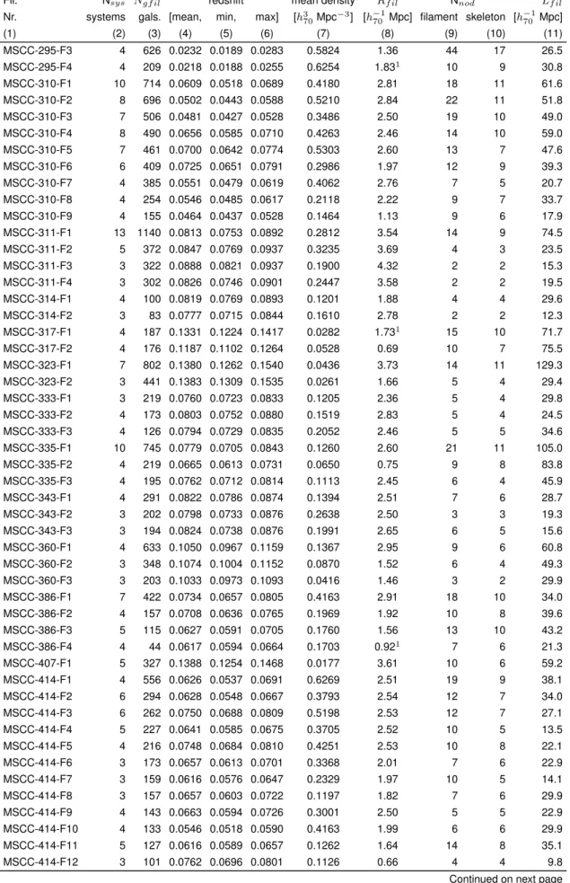
3.4.1 Main properties of the filaments. . . 72
3.4.2 Distribution of galaxies along the filaments . . . 76
3.5 Transversal profiles . . . 77
3.5.1 Density in transversal profiles . . . 78
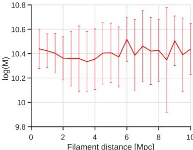
3.6 Properties of galaxies in filaments . . . 81
3.6.1 Stellar mass profile. . . 81
3.6.2 Morphological type . . . 82
3.6.3 Activity type . . . 84
3.6.4 Red sequence analysis . . . 84
3.7 Conclusions . . . 86
4 Characterization of galaxy clusters using SZ 89 4.1 The Planck and ACT sample and SZ data . . . 90
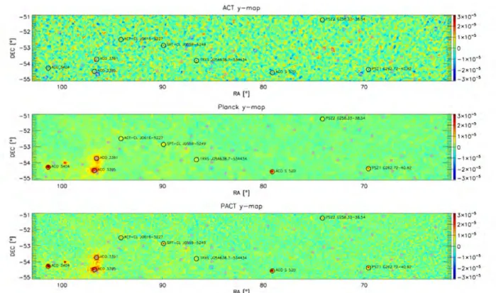
4.1.1 The combined SZ map. . . 90
4.1.2 The cluster sample . . . 90
4.2 Reconstruction of the gas pressure profile . . . 93
4.2.1 Reconstruction of the SZ profile . . . 95
4.2.2 Stacking the y profiles . . . 96
4.2.3 PSF correction and deprojection . . . 96
4.2.4 Stacking pressure profiles . . . 97
4.3 Validation of thePACTprofiles . . . 98
4.3.1 Extraction of profiles from Planck DR2015: from 100 to 70 . 99 4.3.2 Extraction of profiles from Planck DR2015 70: improving the sampling . . . 100
4.3.3 Samples and y-maps: from PLCK to PACT . . . 101
4.4 PACT profiles . . . 102
4.4.1 PACT31 y-profiles . . . 102
4.4.2 Stacked pressure profiles . . . 102
4.5 Conclusions and perspectives . . . 105
Conclusions and Perspectives 107
Conclusiones y perspectivas 110
Conclusions et perspectives 113
A Algorithms 116
Introduction
With the availability of all sky extragalactic surveys, it has been observed that, at large scale, the galaxies (observable baryonic matter) in the Universe are or-ganized in a web-like pattern. This pattern has been observed in several galaxy redshift surveys (e.g. Joeveer & Einasto, 1978; Davis et al., 1982; Shectman et al., 1996; Colless et al., 2001; Huchra et al., 2012). Such observations have shown that the large scale structure (LSS) was composed of elongated filaments, widely spread sheets and higher density knots. The latter are usually located at the intersection of filaments, where clusters and groups are hosted (e.g. Peebles, 1980). According to the current standard cosmological model (e.g. Riess et al., 1998) and observations of the cosmic microwave background (CMB) (e.g. Planck Collaboration et al., 2016b), the Universe is composed of 70% of dark energy and 30% of matter. Of the latter, about 85% is present in the form of cold dark matter (CDM) and only about 15% in the form of baryonic matter.
This model establishes that such structures of matter were formed through grav-itational collapse, in a hierarchical scenario. In other words, the smaller halos (galaxies) formed first, then, they grew by fusion and accretion with other halos. Since the baryonic matter follows, to first order, the distribution of the dark matter, the galaxies and gas populate these structures accordingly (e.g. Eisenstein et al., 2005). The groups and clusters of galaxies are the next step of this hierarchical process of forming the densest regions in the LSS. About 85% of the baryonic matter in these structures is present in the form of hot gas (T ⇠ 107 108K, or kT
⇠ 1–10 keV). This gas can be directly observed by its X-ray emission or through the SZ (Sunyaev–Zel’dovich) effect in the millimeter range. However, theoretical studies (e.g. Cen & Ostriker, 1999) and CMB measurements of the primordial nu-cleosynthesis (e.g. Planck Collaboration et al., 2016b) suggest that, in the local Universe, between one half and two thirds of the baryonic matter has not been detected yet at any wavelength. Nowadays, the results from several numerical
N-body simulations have been used to unveil where these baryons might be lo-cated, e.g. the Millennium (Springel et al., 2005), the Magneticum (Dolag et al., 2016) and Illustris (Vogelsberger et al., 2014). Their results regarding this sub-ject suggest that these baryons might be in a warm and low density gas phase ( T ⇠ 105 107K or kT ⇠ 0.01–1 keV) filling filaments and sheets between galaxy
clusters, constituting the so-called warm hot intergalactic medium (WHIM). The characterization of the WHIM thought observables such as X-rays or SZ effect is very challenging. However, deeper observations and the increase in detec-tion sensitivity at millimetric, optical and X-rays wavelengths open the possibility to better study the dispersed component of the LSS while allowing the following subjects of study:
1. to detect and characterize the LSS components (e.g. topology, density, tem-perature, dynamical state, matter distribution and its evolution with time), 2. to better constrain the environment role in galaxy evolution,
3. to understand the mechanisms that shape the LSS matter distribution and 4. to evaluate and improve the current standard cosmological model.
In this framework, this Thesis is focused on studying the first and second sub-jects, characterizing the LSS components and investigating their effects on the galaxies evolution. By this, we aim to understand the mechanisms driving the LSS distribution, the third subject. Firstly, we present the characterization of LSS components (filaments, groups and clusters) along with the study of their envi-ronmental effects on the galaxy properties. Secondly, we present the charac-terization of galaxy clusters through the extraction of intra-cluster medium (ICM) pressure profiles from a high resolution SZ map.
In Chapter 1, we describe briefly the cosmological context that is used for our work and we introduce the current state of the art regarding the LSS components: galaxy clusters and filaments.
In Chapter 2, we introduce a general view of the current advances in detection of the disperse component of the LSS. Then, we describe in detail the method-ology we implemented for the detection of clusters and filamentary structures. Our method aims the detection of chain-like structures inside a sample of galaxy superclusters (from Chow-Martinez et al., 2014) in the Local Universe (z ⇠ 0.15).
As shown in Tanaka et al. (2007), the possibility to find elongated chain-like struc-tures increases in superclusters.
In Chapter 3 we present the analyses we carried out to search for correlations between the galaxy properties (mass, morphology, activity, color and metallicity) and the environment in which these galaxies reside. For this analysis we used the Sloan Digital Sky Survey (SDSS) spectroscopic redshifts and sub-products (Albareti et al., 2017).
Chapter 4 is orientated towards the study of the gas component of galaxy clus-ters. We describe the methodology used for reconstructing the 3D radial profile of the thermal pressure for a sample of clusters, and the statistical analysis of the pressure distribution across the sample. These analyses were achieved us-ing a composed SZ map from Planck and ACT (Atacama Cosmology Telescope) surveys,PACTmap (Aghanim et al., 2019a).
The final Chapter of this Thesis discusses the results of this work regarding the detection of LSS structures, their classification and characterization. We review the trends and correlations observed for galaxies inhabiting different components of the LSS detected by our algorithms, and discuss the possible environmental effects over their evolution. In addition, we discuss different approaches to carry out further analyses of the characterization of the gas component of clusters and filaments, in a similar way as the study carried out in this Thesis, using the SZ effect. We also discuss the achievements of, and our contribution to the LSS structure detection algorithms. Finally, the directions for further characterization of the LSS components using optical and gas components are presented. We also describe the future applications of the GSyF and GFiF algorithms. For this work we adopt (H0, ⌦M, ⌦⇤, ⌦k, ⌦r) = (0.7, 0.3, 0.7, 0.0, 0.0).
Chapter 1
A Cosmology context
The different theories formulated in the history of cosmology aim to bring under-standing on the mechanisms that govern the formation and distribution of matter and energy in the Universe. As the observational facilities provide deeper and more sensitive observations, in different wavelength regimes, the cosmological theories need to be improved in order to model the Universe as observed today. The study and characterization of the LSS distribution and its content through observables can be used to evaluate the cosmological models and see if they reproduce what is observed.
In this Chapter we present the principal aspects of the cosmology formalism that are behind the most accepted cosmological model and introduce the current state of art regarding the study of the main components of the LSS.
1.1 The standard cosmological model
1.1.1 The establishment of the ⇤CDM model
The standard cosmological model, ⇤CDM (e.g. Bond & Szalay, 1983; Doroshke-vich & Khlopov, 1984), sometimes referred to as the concordance model, was motivated by observational studies of the LSS and the observations of the CMB. As summarized by Battaner & Florido (2000), Einasto (2009) and Einasto (2014), the cosmological model has changed to adapt to the observational facts along
with the new theories about structure formation; here we introduce the most im-portant contributions to this cosmological model. At the beginning the model sug-gested the hypothesis that the first galaxies were formed from primordial density fluctuations of the baryonic medium (Harrison, 1970). However, there were prob-lems with physical and kinematic properties of galaxies and clusters such as the potential energy needed to keep these structures bounded (Oort, 1940; Roberts, 1966; Rubin & Ford, 1970). Then, to explain these discrepancies, a dark matter in the form of dark stellar population and gaseous halos was proposed (e.g Os-triker & Peebles, 1973; Bahcall & Casertano, 1985). With the first observations of the CMB the model was discarded since the observed density fluctuations were smaller than predicted. As an alternative, the Hot Dark Matter model was pro-posed. This model suggested a non-baryonic relativistic neutrino-like particle as candidate for the dark matter, which explained the small fluctuations observed in the CMB (Cowsik & McClelland, 1973; Szalay & Marx, 1976; Tremaine & Gunn, 1979; Doroshkevich et al., 1980; Chernin, 1981). However, in this scenario, the structures observed today would not have had enough time to build up and the model was also abandoned. This gave place to a new hypothetical dark matter particle which moves slowly leading place for structure formation. This model was called Cold Dark Matter (CDM) (Blumenthal et al., 1982; Bond et al., 1982; Peebles, 1982; Pagels & Primack, 1982; Doroshkevich & Khlopov, 1984). It was originally proposed as a theory opposed to the Hot Dark matter (HDM) neutrino model. Finally, supernovae observations showed that the Universe was in a state of accelerated expansion. This brought up the need for a return of the cosmolog-ical constant ⇤, see Section1.1.3, to open space for a supposed vacuum energy, leading to the current ⇤CDM model.
1.1.2 The fundamental parameters
Considering the expansion of the Universe is uniform, the distance and velocity of an object can be expressed as:
r(t) = a(t)⇥ DC(t), (1.1)
where DC(t) is the comoving distance, H(t) the Hubble parameter and a(t) the
scale factor. The expansion rate is dictated by the term = H(t)r(t) which re-lates the separation and recession velocity of distant galaxies. Then, the Hubble-Lemaˆıtre law is approximated to:
v(t) = H(t)DC(t), (1.3)
for the Local Universe. By convention, the sub-index 0 denotes the current value for the Hubble parameter at z = 0, usually written as H0 = 100 hkm s 1Mpc 1,
scaled in terms of h. For instance, Planck Collaboration et al. (2016b) measured h as 0.6772 ± 0.0046 using CMB measurements, while the Gaia mission mea-sured a value of 0.7348 ± 0.0166 using a distance scale derived from Cepheid parallaxes (Riess et al., 2016). Another approach by Cuceu et al. (2019) mea-sured h = 0.676 ± 0.011 using Baryon Acoustic Oscillations, while the H0LiCOW collaboration (e.g. Suyu et al., 2017) measured h = 0.733 ± 0.0175 using the time delay of lensed quasars. Another interesting result was the measurement by Ho-tokezaka et al. (2019) using the radio counterpart of GW170817, combined with gravitational wave and electromagnetic data, h = 0.703±0.0515. Considering that the Universe is isotropic at large scale and has a constant curvature, then, the space-time can be expressed by the Friedman-Robertson-Walker metric which, in spherical coordinates, is written as:
ds2 = c2dt2+ a2(t) ✓ dr2 1 kr2 + r 2d⌦2 ◆ , (1.4)
with a2 > 0and ⌦2 = d✓2+ sin2✓d 2. k determines the space curvature as:
k 8 > > > < > > > :
> 0 the space-time is closed (spherical-like topology), = 0 the space-time is flat,
> 0 the space-time is open (hyperbolical-like topology).
Then, a useful observational measurement to estimate an object’s distance is the redshift. The redshift is the result of the Doppler effect seen in the the galaxies optical spectra or magnitude, consequence of the expansion of space in all di-rections. Measuring the redshift of the spectral lines allow us to estimate when the light photons were emitted. The time between an object emitting photons and
the observation can be defined as: Z tobs tsource = c dt a(t) = Z tobs+ obs/c tsource+ source/c c dt a(t), (1.5)
Then, the redshift is deduced as: vsource
vobs
= aobs asource
= 1 + z, (1.6)
with vsource the velocity of the object and vobs observed velocity. For small
red-shifts, i.e. small distances, we can approximate z ⇠ vsource
c .
1.1.3 Dynamics of a Universe in expansion
Considering that the Universe is homogeneous and isotropic, its evolution can be described, in General Relativity, by the Friedmann-Lemaˆıtre Equations:
(˙a a) 2 = 8⇡ G 3 ⇢tot kc2 a2 +⇤c 2 3 (1.7) ˙a a = 4⇡G 3 ⇢tot+ 3ptot c2 with (1.8) ⇢tot = ⇢⇤+ ⇢m+ ⇢r, (1.9)
where ⇢⇤ = ⇤/8⇡G corresponds to the dark energy contribution. Here ⇤ is the
cosmological constant1, ⇢
m = ⇢c+ ⇢b corresponds to the matter density (where ⇢b
is the baryonic density and ⇢c is the dark matter density); the density of radiation
is ⇢r while k is the Universe curvature. A detailed derivation of Equation1.7from
Einstein’s equation can be consulted in Padmanabhan (2003).
Then, the density and pressure can be expressed in terms of the cosmological constant as: ⇢! ⇢ + ⇤c 2 8⇡G and p ! p ⇤c2 8⇡G. (1.10)
and the Friedmann equations can be re-written in terms of energy density of pressure: H2 = ✓ ˙a a ◆2 = 8⇡ G 3 ⇢tot kc2 a2 , (1.11)
1Introduced by Einstein in 1917 to compensate the natural dynamics (expansion or
contrac-tion) of the Universe and make it static. Currently it is used to represent the dark or vacuum energy effect which causes an acceleration in the expansion of the Universe.
Considering Equation 1.11 with k = 0, i.e. a flat Universe, we can derive the critical density of the Universe as ⇢c = 3H
2 0
8⇡G. The density parameter can be written
in terms of the critical density as: ⌦ = ⇢(t)/⇢c(t).
Then the ⇢⇤, ⇢m and ⇢r can be re-written in terms of the density parameter
(Pee-bles, 1993): ⌦m= 8⇡G⇢tot 3H2 0 , ⌦k= k a2H2 0 , and ⌦⇤= ⇤ 3H2 0 (1.12) The Friedmann equation can be re-written in terms of the density parameter as:
⌦m+ ⌦r+ ⌦⇤+ ⌦k = 1 (1.13)
Then the curvature of the Universe can be defined as:
kc2 = a20H02(⌦tot 1) = a02H02(⌦m+ ⌦r+ ⌦⇤) (1.14)
Considering Equations1.7, the fluid equation of state can be expressed as:
˙⇢ + 3H⇣⇢tot+
ptot
c2
⌘
= 0, (1.15)
In order to simplify, the pressure and energy can be related by p = p(⇢). The Equation1.15can be solved for a fluid with no torsion considering p = w⇢, where w = ( 1)is constant and ⇢ / a 3(1+w), leading to the solution of the Friedman
Equation of the form a / t2/( 3(1+w)).
This solution can be used to estimate the evolution of energy density:
The Radiation dominated Universe: called Tolman Universe; it is defined by w = 1/3and a radiation density ⌦r ⇡ 1. Then the density and scale factor evolve as:
⇢r(t) = ⇢r0 ⇣a0 a ⌘4 with a(t) = a0 ✓ t t0 ◆1/2 (1.16) Matter dominated Universe: if w = 0 then p = 0 then matter is pressureless, corresponding to the Einstein-de Sitter Universe with the values of energy density and scale factor:
TABLE 1.1: Cosmological parameters. h 0.6772, 100 ⌦⇤ 69.11± 0.62, 100 ⌦m 30.89± 0.62, 100 ⌦ch2 11.88± 0.10, 100 ⌦bh2 2.23± 0.014, 100 ⌦r 5⇥ 10 3, 100 ⌦k 0.00± 0.50. ⇢m(t) = ⇢m0 ⇣a0 a ⌘3 with a(t) = a0 ✓ t t0 ◆2/3 (1.17) Curvature dominated Universe: In the case of an open Universe with k < 0, the Equation1.7does not have a solution, then:
⇣a0 a ⌘2 = k a2 with a(t)/ a0 ✓ t t0 ◆ . (1.18)
Energy dominated Universe: this is called de Sitter Universe. With w = 1 the scale factor has to be expanded by a Taylor series.
⇢⇤(t) = ⇢0 with a(t) = a0eH(t t0). (1.19)
Combining Equations 1.6, 1.14 and 1.13, the Friedmann equation now can be expressed in terms of redshift and densities as:
H2 = H02(⌦r(1 + z)4+ ⌦m(1 + z)3+ ⌦k(1 + z)2 + ⌦⇤), (1.20)
Values of these densities have been recently measured using observations of the Planck satellite (Planck Collaboration et al., 2016b) results:
From the latter, we can highlight that, according to the ⇤CDM cosmological model, the Universe is predominately composed of dark energy while its mat-ter content is mainly composed of cold dark matmat-ter, its curvature is flat and it is in a state of accelerating expansion.
1.1.4 Distance measurements in the Universe
Comoving distance in the line of sight Considering two objects moving with the Hubble flow, the measurement of the distance between them (proper dis-tance) at different times needs to be scaled. The distance from us to an object in the line of sight, the comoving distance DC, is defined as:
DC = c H0 Z z 0 dz0 E(z0), (1.21) DC = DH Z z 0 dz0 E(z0), (1.22)
with E(z), defined by Peebles (1993), as: E(z) = H(z)
H0
=p⌦r(1 + z)4+ ⌦m(1 + z)3+ ⌦k(1 + z)2+ ⌦⇤, (1.23) Angular diameter distance and luminosity distances The angular diameter distance DA is used to measure the actual size of objects observed with small
angular sizes ( ✓), that is, separations perpendicular to the line of sight, defined as ✓ ⇥ DA. The angular diameter distance is used to convert from angular
distances in physical separations and has the form: DA =
Dm
1 + z. (1.24)
where Dmis the comoving angular diameter distance which depends on the
Uni-verse curvature and is defined as:
Dm 8 > > > > < > > > > : DHp1⌦k sinh ⇣p ⌦kDDCH ⌘ for ⌦k > 0, DC for ⌦k = 0, DHp1⌦k sin ⇣p ⌦kDDCH ⌘ for ⌦k < 0,
Another useful distance measure is the luminosity distance which, in an expand-ing space, can be defined as:
D2L= Ls
4⇡F, (1.25)
where F is the flux received from an emitting source with absolute luminosity Ls.
as:
DL = (1 + z)Dm = (1 + z)2DA. (1.26)
1.2 The Universe’s thermal history
The combination of observations, the cosmological model and particles physics, allows us to study the early Universe by reconstructing the evolution of its com-ponents.
The Planck Era: T ⇠> 1032 K According to the current cosmological model, at
the beginning the Universe was in an extremely hot, dense and in ionized state. The study of the evolution of the Universe allows one to reconstruct its thermal history up to the so-called Planck’s time, tp = 10 43 seconds after the Big Bang.
Before this time, quantum corrections become significant due to the extreme tem-perature, and density. At this moment the gravity ional force separated from the other forces. This corresponds to the moment at which the de Broglie wavelength of the Universe equals to its Schwarzschild radius:
~ mc =
2Gm
c2 (1.27)
The GUT Era: T ⇠ 1032 1029 K At z ⇠ 1032, t ⇠ 10 43 10 36s the GUT
the-ories propose a model in which the asymmetry between matter and antimatter produce a phase transition. This transition makes the Universe expand expo-nentially, giving rise to the inflation theory (Starobinsky, 1980; Guth & Pi, 1982; Linde, 1982).This model gives a solution to the so called homogeneity problem, allowing the formation of the structures observed today from primordial density inhomogeneities, at a Hubble radius.
The particle Era: T ⇠ 1015 109 K When the Universe cools to a temperature
about T ⇠ 1016 K, (t ⇠ 10 12s 2 min) the electromagnetic and nuclear weak
forces separate. At this point the quarks, electrons, photons and gluons form a plasma in constant interaction. Afterwards, as the temperature decreases, at
about T ⇠ 1013 K, the strong nuclear force allow the transition between quarks
and hadrons, forming the protons and neutrons.
The primordial nucleosynthesis: T ⇠ 1016K The neutrinos and anti-neutrinos
stop their interactions with electrons. As the baryons cooled, at temperatures about T ⇠ 109K, the first deuterium and helium nuclei were formed. This
pro-cess is called primordial nucleosynthesis and depends on the expansion rate of the Universe. This processes also determines the amount of baryonic matter in the Universe, which is measured to be between 4% and 5% of the critical density of the Universe.
In the Big Bang Model, nucleosynthesis occurs in the radiation-dominated epoch. The density of the Universe can be estimated as function of the temperature as ⇢(T ) = (⇡2/30)N
relT4, where Nrel is the effective number of bosonic degrees of
freedom. Under this scenario: when a(t) ! 0, the density ⇢ ! 1 and T ! 1. However, the primordial densities can be calculated assuming that the reaction:
p + e ! n + ⌫e, (1.28)
occurs in thermal equilibrium, such that the interaction rate, (t) = nh ⌧vrmsi
(where ⌧ is the Thomson cross section and vrms is the rms velocity), allows
hydrogen to form.
Photon decoupling and recombination: T ⇠ 104 K At this temperature the
Universe is dominated by relativistic particles and the matter and radiation den-sities are in equilibrium (t⇠ 47kyr,T⇠ 104K, z⇡ 3600). Then, at temperatures of
⇠ 3 000 K the electrons combine with nuclei to form stable neutral atoms. At this moment, the photons decouple from the matter in all directions, as evidenced by the cosmic microwave background (CMB), See Section1.3. One can define the temperature of the primordial photons at the moment of decoupling from the matter, dependent on the expansion as:
T (t)/ 1
a(t). (1.29)
The dark era and the formation of the first stars: T ⇠ 15 K The CMB
of gravity the first dark matter halos formed the first galaxies which agglomerated giving plate to the first galaxy clusters following a hierarchical structure formation scenario. Moreover, clouds of gas formed under the effect of gravity inside these halos, giving place to the first stars giving place to the reionization Era (T⇠ 60-19 K, 200Myr, 20>z>6).
1.3 The cosmic microwave background
The cosmic microwave background (CMB) was first observed by accident by Pen-zias & Wilson (1965) while carrying out an observation for radio emission. Thanks to their discovery they were awarded with the Nobel prize in 1978. The CMB is observed as an isotropic emission in the microwave window, coming from all di-rections in the sky. Its power spectrum represents the Universe a little bit after the moment at which matter and radiation density were equal.
1.3.1 CMB electromagnetic spectrum
The CMB photons are uniformly distributed and have a temperature of 2.725 ± 0.00335K (Fixsen, 2009) with a black body spectrum defined as:
B⌫(TCM B) = 2h⌫ c2 ✓ 1 exp ✓ h⌫ kBTCM B ◆◆ 1 [Wm 2sr 1Hz 1], (1.30) where h and kBare the Planck and Boltzmann constants, respectively. The CMB
observations suggest that the photons were indeed very close to equilibrium at some point in the early Universe. However, the CMB temperature presents small fluctuations (anisotropies) of the order TCM B = (T hT i)/hT i ⇠ 10 5.
1.3.2 CMB angular power spectra
In general, the anisotropies of the CMB are quantified by their power spectrum. These anisotropies are observed as a function of direction over the celestial sphere. Therefore, they are expressed in terms of spherical harmonics:
T (ˆn) = 1 X `=0 ` X m= ` T`mY`m(ˆn) (1.31)
where ˆn is the direction of observation. The multipole index ` quantifies the scale (long wavelength modes corresponding to low values of `). The CMB power spectrum as a function of ` is defined as:
C` =h|T`m|2i (1.32)
The anisotropies of the CMB contain information of the primordial density fluc-tuations in the early epoch of the Universe. In addition, CMB photons, on their trajectory across the Universe, have been perturbed by gravitational potentials or scattered by inverse Compton effect with ionized media. Such interactions are called secondary perturbations. The Sachs-Wolfe effect is attributed to tempo-ral variation of the gravitational potential along the photon trajectory (Sachs & Wolfe, 1967). Other anisotropies observed are attributed to gravitational lenses (Planck Collaboration et al., 2018). In this case, anisotropies are generated by the change on the trajectory of photons due to the gravitational potential of a very massive object, like galaxy clusters. Another gravitational effect, called the Rees-Sciama effect (Rees & Rees-Sciama, 1968), can induce anisotropies in the CMB due to evolving gravitational potentials of non linear or matter structures as a result of collapse or expansion. Moreover, along their journey through the Universe, the CMB photons also interact with the gas in galaxy clusters, via the Sunyaev-Zel’dovich effect (Sunyaev-Zel’dovich, 1970; Sunyaev & Zeldovich, 1972). This interaction is of particular interest for the study of galaxy clusters and will be discussed with more detail in Section1.4.4.
The peak in the CMB power spectrum observed at ` ⇡ 200 in the power spec-trum (corresponding to an angular size of about 1 ) represents the largest scale that had time to collapse at recombination. At smaller values of `( 50), corre-sponding to very large scales, the spectrum is flat, which is just proportional to the nearly scale-invariant spectrum at the moment fluctuations cross the Hubble radius.
Figure 1.1 shows the angular power spectrum of the CMB as measured by the Planck satellite (Planck Collaboration et al., 2016b). The vertical axis of the CMB power spectrum correspond to `(` + 1)C`, this is proportional to the square of the
FIGURE 1.1: Power spectrum of the CMB as measured form Planck DR15
re-sults. Figure extracted from Planck Collaboration et al. (2016b).
temperature fluctuations on the angular scale, ✓ ⇡ ⇡/`. In this representation, the CMB spectrum is about flat at large scales, ` < 50.
1.4 The Large Scale Structure
1.4.1 Primordial overdensities and structure formation
In the ⇤CDM model, the initial state of perturbations is assumed to be adiabatic and scalar. Such perturbations grow under the effects of gravity, leading to the formation of structures. These overdensities are measured in terms of the density contrast:
= ⇢(ˆr, t) ⇢¯bg(t) ¯
⇢bg(t)
, (1.33)
with ¯⇢bg(t)representing the mean background density measured at a time t.
Con-sidering only the contribution of gravity (Kaiser, 1986) in a Universe with ⌦tot = 1,
the spectrum of density fluctuations may be written as:
Considering k / 1/r and M / r3, the mass variance of fluctuations, 2, can be
expressed as:
2(k)⇠ k3P (k)/ r (n+3) ⇠ M (n+3)/3 (1.35)
Under these assumptions, by definition the fluctuations are self similar. How-ever, as mentioned by Kaiser (1986), this property can only be applied at cluster scales, allowing to construct scaling relations, which are discussed in section
1.4.4.
Observations of the CMB power spectrum, as mentioned above, provide direct evidence of primordial perturbations. The initial density perturbations can be represented by Gaussian samples with mean zero, i.e. h i = 0, then the power spectrum is given by:
P (t, k) =h| k(t)|2i (1.36)
where k is the Fourier transform of (t, ˆr). A complete characterization of the
density perturbations at the time of decoupling is given by the CMB the power spectrum: P (k) = Z (ˆr) exp ikˆrd3x = 4⇡ Z (R)sin(kR) kR r 2dR (1.37)
The spectrum is computed, when the density contrast is low, assuming a linear perturbation. However, when ⇠ 1 analytical solutions are needed, some ex-amples of such solutions can be consulted in Padmanabhan (2002). This model is called spherical top-hat approximation. The linear density contrast can be de-rived from solving Equation 1.33 in the regime of nonlinear perturbations, in a matter dominated Universe and it is defined as:
L= 3 5 ✓ 3 4 ◆2/3 (✓ sin ✓)2/3. (1.38) Figure1.2depicts the density as calculated from Equation1.38. At the beginning, the perturbed region detaches from the cosmic expansion, starting to expand at lower rate. One can observe that at ✓ = 2⇡/3 the solution is no longer linear. Afterwards, at ✓ = ⇡ the matter collapses after the so-called turnaround point. Finally, bounded structures are formed at ✓ larger than 2⇡.
Now, if the density fluctuations are very small, << 1, then the solution to Equa-tion 1.33 is non-linear and is then solved by an analytic model developed by Press & Schechter (1974), see Percival (2001) for details. Then the variance of
FIGURE1.2: Evolution of an overdense region in a spherical top-hat
approxima-tion. Here anl refers to non-lineal and acoll to collapse. Figure extracted from Padmanabhan (2002).
the mass fluctuations is given by: (R)2 =
Z k2
(2⇡)2W 2
s(kR)P (k) dk, (1.39)
where Ws is the top-hat filter in the Fourier space defining spheres of radius
R. The amplitude of the power spectrum on the scale of 8 h 1
70 Mpc is called 8, defined as the r.m.s. density variation when a top-hat filter of 8 h701Mpc is
applied. It can be expressed as:
8 =
1 2⇡2
Z
W k2P (k) dk, (1.40) where Ws is the top-hat filter in the Fourier space:
Ws=
3j1(kRs)
kRs
, (1.41)
1.4.2 Supercluster of galaxies
The Large Scale Structure (LSS) of the Universe, as observed today, shows a web-like pattern formed by groups and clusters of galaxies, elongated filaments, widely spread sheets, and voids (e.g. Peebles, 1980; Davis et al., 1982; Bond et al., 1996). The superclusters of galaxies are individual fragments of this LSS, forming sheets or just a weblike structure connecting filaments. The nodes where these filaments cross are the focus of clusters and groups of galaxies. Thus, su-perclusters of galaxies can be defined as the largest and most massive structures ongoing gravitational effects, although they are not virialized. They probably just passed the quasi non-linear regime described by the Zel’dovich’ approximation (1970, see also the “sticking model” by Shandarin & Zel’dovich 1989), and may be close in time to the turn around point. As a consequence, the inter-cluster medium embedded in them (dark halos, gas and galaxies) dynamically interacts and organizes by falling in to the gravitational potential of the massive halos, forming bridges between pairs of clusters and groups.
Superclusters can be identified from groups of clusters of galaxies (e.g. Abell, 1961; Zucca et al., 1993; Einasto et al., 2001; Chow-Martinez et al., 2014) but also from the galaxies distribution, their local density and luminosity (e.g. Lu-parello et al., 2011; Costa-Duarte et al., 2011; Liivam¨agi et al., 2012). Recent numerical N-body simulations based on the ⇤CDM cosmological model (e.g. Mil-lennium, Springel et al., 2005; Bolshoi, Klypin et al., 2011; Illustris, Vogelsberger et al., 2014) reinforce that these structures are assembled under the effect of gravity and the process of gravitational collapse is still ongoing.
1.4.3 Galaxy clusters
Since 85% of the ICM is present in the form of hot gas, observations of such gas may be subject of study in order to characterize the ICM of clusters. There exist multiple studies of the ICM carried out through X-ray and SZ observations (e.g. Arnaud et al. (2001); Pointecouteau et al. (2005); Croston et al. (2008); Arnaud et al. (2010a); Planck Collaboration et al. (2011, 2013a); Bourdin et al. (2017)). These studies present analyses of the gas density, temperature and pressure of the ICM which confirm the strong similarity, in shape, of the clusters. There exist several models to estimate the mass distribution of galaxy clusters using
different observables. In the following paragraphs some examples used to model the clusters’ density profiles are presented.
The isothermal sphere The distribution of galaxies in the central region of rich
clusters can be approximated by the King distribution, (King, 1972): ngal = n0gal ✓ 1 + r Rc ◆ 3/2 , (1.42)
with Rc the core radius and n0gal the central density. However, the mass estimated
from this model diverges when r 0 and r 1. Moreover, observations of galaxy clusters suggest that the velocity dispersion of galaxies is proportional to their distance from the cluster center. This leads to the analytical model of an isothermal sphere with a density distribution of the shape:
⇢(r) =
2 v
2⇡Gr2. (1.43)
This model, originally proposed to estimate the dark matter profile for a self-gravitating isothermal sphere (as detailed by Binney & Tremaine, 1987), is used to estimate the cluster properties in analytical analyses.
S´ersic profile The S´ersic profile, (S´ersic, 1968) is a surface brightness 2D profile for galaxies. It is defined by:
⇢(r) = ⇢sexp( bn[
r rs
]1/n 1). (1.44)
where ⇢s is the surface brightness at radius rs, measured at the half bright
sur-face. The parameter bn can be approximated as 2n 1/3, as shown by Ciotti &
Bertin (1999), where n describes the shape of the light profile.
Beta profile Regarding the gas component of galaxy clusters, the density pro-file can be computed considering the beta propro-file (Cavaliere & Fusco-Femiano, 1976). This profile is a modified profile adapted for the distribution of gas. Here
the gas distribution is given as: ⇢gas(r) = ⇢go " 1 + ✓ r rc ◆2# 3 /2 , (1.45) with = µmp 2 kTg . (1.46)
Navarro-Frenk and White cluster profile Numerical simulations of structure formation have provided a solid description of the gas behaviour under the in-fluence of the key physical processes governing the intra-cluster medium (ICM Nagai et al., 2007; Battaglia et al., 2010). The dark matter density profile of galaxy clusters is approximated by a Navarro-Frenk and White profile, (Navarro et al., 1997, hereafter, NFW):
⇢(r) = c⇢c (r/rs)(1 + r/rs)2
(1.47) where ⇢c is the critical density at the cluster redshift, rs is the scaled radius found
by Navarro et al. (1997) and c is the characteristic density (for a concentration
parameter c) defined as:
c =
200 3
c3
ln(1 + c) c/(1 + c) (1.48) Usually this profile is adjusted using an analytical solution of the NFW profile parametrized as:
⇢(r) = c⇢c0 x (1 + c↵
500x)( )/↵
, (1.49)
where ↵, and are the best fitted slopes for the density profile.
The generalisation of the Navarro et al. (1997) profile (gNFW) for the distribution of dark matter and gas derived from early numerical simulations, as given by Nagai et al. (2007) is:
P(x) = P0
(c500x) [1 + (c500x)↵]( )/↵
where x = r/rs, rs = r500/c500. r500 and c500 are the characteristic radius and the
corresponding concentration encompassing 500 times the critical density of the Universe at the cluster redshift . ↵, and are the inner, external and transition slopes (at rs) of the profile. The gNFW profile thus provides a simple parametric
description easily tested against observational constraints (e.g., Arnaud et al., 2010b; Planck Collaboration et al., 2013a; Eckert et al., 2013; Sayers et al., 2016; Romero et al., 2017; Bourdin et al., 2017; Ruppin et al., 2018). The afore-cited works have found a very good agreement between the gNFW predictions and the actually observed pressure distribution in X-ray or SZ, at least within the central part of the galaxy clusters.
1.4.3.1 The X-ray observations
As mentioned before, the ICM gas is observed to have temperatures of about 108K, corresponding to 1-30 keV. This gas cools by thermal Bremsstrahlung
emis-sion which depends quadratically of the gas density ne. Then, the X-ray surface
brightness is used to estimate the gas density. The X-ray surface brightness by unit of solid angle is given by:
Sx =
1 4⇡(1 + z)4
Z
ne⇤(Te, Z)dl, (1.51)
where dl refers to the line of sight, ⇤(Te, Z)is the cooling function which depends
on the gas metallicity, Z and the temperature Te. ⇤(Te, Z)can be approximated as
p
Te Although the X-ray emission is suitable to characterize the ICM gas density
and its metallicity, it depends on the cluster’ density, then, at lower densities, photon detection requires larger observation times. Also, its redshift dependence makes it difficult to detect and characterize clusters at large redshift. Therefore, clusters can be studied using X-ray observations only in their densest region, i.e. close to the core. Analyses up to the cluster outskirts have as a consequence an increment in the observation time, also, the required instrumentation sensitivity increases, making such studies very challenging.
1.4.4 Scaling relations
In the hierarchical structure formation scenario, galaxy clusters are the largest gravitationally bounded structures. One can consider the hypothesis that clusters evolved purely by gravitational collapse, following a spherical collapse model, as proposed by Jeans (1902). Then, by assuming these systems are virialized, the matter contained in their gravitational potential will be in hydrostatic equilibrium. Also, one can assume the gas fraction in clusters, fgas = Mgas/Mvir is constant
and representative of that of the Universe. Therefore, as a consequence of these approximations, galaxy clusters and groups halos have self-similar internal struc-ture. This property allows to construct scaling relations between the cluster prin-cipal properties (Kaiser et al., 1995; Bertschinger, 1998).
This behaviour is observed for their global thermodynamical properties (e.g., Gio-dini et al., 2013a) as for their internal distribution (e.g., Pratt et al., 2019). The gas thermal pressure is a remarkable example of this self-similar behaviour. The integrated pressure over the volume of the cluster, i.e., the SZ Comptonization parameter, has proven to be an excellent proxy of the total gas content, thus of the total mass of the halo, as the thermal pressure is mildly affected by non-gravitational physics (AGN feedback, radiation cooling, etc) with respect to other proxies (e.g., X-ray total luminosity Pratt et al., 2019; Mroczkowski et al., 2019, for recent reviews).
Let us consider a spherical region of radius R cwith a mean density of c⇢c(z)at
redshift z. The total mass is given by M c = (4⇡/3) c⇢c(z)R3c. The critical
den-sity is defined at any redshift as ⇢c(z) = ⇢c0E(z), with E(z) as defined in Equation 1.23. Then the cluster radius as function of redshift can be approximated as:
R c / M
1/3
c F
(2/3)
z . (1.52)
with Fz the source flux. Now, considering the gas in clusters satisfies kBT /
, M c/R c, then we have:
M c / T
3/2F 1
z . (1.53)
This last equation can be used to derive scaling relations from X-ray observables. These relations generally link by a power law the cluster mass with a measured proxy (e.g. the luminosity, gas temperature or the galaxies’ velocity dispersion).
Some of the most used scaling relations are between X-ray luminosity and tem-perature, mass and temperature and luminosity-mass relations (e.g. Ettori et al., 2004; Arnaud et al., 2005; Kotov & Vikhlinin, 2005; Pratt et al., 2009; Giodini et al., 2013b, the latter provides a review regarding scaling relations for clusters):
FzMgas / T3/2, (1.54)
F 1
z Lx / T2, (1.55)
Fz 1Lx / (FzMgas)4/3, (1.56)
Fz4/3Sx / T, (1.57)
However, it is important to recall that scaling relations are a consequence of the assumption of hydrostatic equilibrium. In a more realistic scenario, the dynamical state of the clusters at radii larger than R500 ( c = 500) is perturbed by accretion
of the infalling material from the filaments and dynamical interactions. Then, in this region one can no longer consider the gas to be in a virialized state. Thus, the characterization of the gas in the cluster outskirts is a crucial step to understand the formation and evolution of these structures.
The SZ effect observations The Sunyaev-Zel’dovich (SZ) effect is a result due to the inverse Compton effect between the hot electrons in the ICM and the photons of the CMB. As a result of this interaction, the spectrum of the CMB shows a deformation toward the regions of clusters.
The intensity of the SZ effect is characterized by the dimensionless Comptonisa-tion parameter y. As defined in Planck CollaboraComptonisa-tion Int. V (2013), the Comp-tonisation parameter corresponds to the product of the average fractional energy transferred per collision, by an electron to a photon, and the average number of collisions, such that:
y = T mec2
Z
P (l)dl, (1.58)
Then the SZ flux expressed as the integrated Compton parameter, Y , within a given solid angle, ⌦, is proportional to the thermal pressure of the ICM gas inte-grated over the line of sight:
Y (⌦) = T mec2 Z ⌦ d⌦ Z los P (l) dl (1.59)
where T is the Thomson cross-section, me is the mass of the electron, c is the
speed of light and P is the pressure produced by the plasma of thermal electrons along the line of sight. Since the SZ effect is independent of the distance of the object to the observer, the SZ effect is related to the redshift only by the angular size at which the cluster is observed. The virial approximation for galaxy clusters is:
kBTe = µmp
GMtot
R , (1.60)
where Mtot is the mas comprised in a sphere of radius R and is a mass
dis-tribution factor and µ the molecular mass of ICM particles. Then, assuming the ICM gas can be approximated as an ideal gas, the Y M relation is:
Y (R )/ ⌧ mec2 ⌫ ⌫e ✓ G2H(z)2 16 ◆1/3 fgasMtot, 5/4, (1.61)
where e the electron mass, fgas is the ratio of the ICM gass mass to the total
cluster mass, which is assumed to be constant.
As a complement to X-ray observations, SZ observations offer the possibility to study the integrated pressure over statistically significant samples of clusters (e.g. Planck Collaboration X, 2011; Planck Collaboration Int. III, 2013; Czakon et al., 2015; Bender et al., 2016; Dietrich et al., 2019) demonstrating a coher-ent view of their gas contcoher-ent between X-ray and millimetre measuremcoher-ents. The increasing coverage and improving resolution and sensitivity of SZ observations have also allowed to constrain the pressure distribution over the whole volume of clusters (Plagge et al., 2010; Planck Collaboration et al., 2013a; Sayers et al., 2013; Eckert et al., 2013).
Plagge et al. (2010) extracted the pressure profiles of 15 clusters up to 2 ⇥ R500
using the South Pole Telescope. Their analysis shows a consistency with the X-ray cluster parameters. Planck Collaboration et al. (2013a) presented an analysis of the extracted SZ signal from the Planck satellite for 62 clusters. Their results combine X-rays for r < R500 and SZ signal for r > R500 to extract the pressure
profiles up to 3 ⇥ R500. Another study carried out by Bourdin et al. (2017) used the
Planck full mission data to extract the pressure profiles for two samples of galaxy clusters, 61 clusters at z⇠ 0.15 and 23 clusters at z⇠ 0.56. They combined X-ray for the inner part of the clusters and SZ for the outskirts.
1.4.5 The dispersed component of superclusters and the
fila-ments
Filamentary structures in superclusters are observed between galaxy clusters forming bridges of galaxies or, at larger scales, composing chains of clusters. The complex morphology of superclusters has been studied previously by several authors. Basilakos et al. (2001) studied the supercluster morphology using a differential geometry definition of shape. Their results suggest that filamentary morphology was the dominant feature for their supercluster sample. Moreover, Costa-Duarte et al. (2011) found, using Minkowsky functionals, that half of their sample have a pancake morphology while the other half exhibited filamentary morphology.
Due to its relatively low density and temperature, the WHIM is very difficult to ob-serve with the current observational facilities (in X-rays and SZ effect). However, there exist some observational evidence of a WHIM in filaments. Among the best studied cases are the pairs of clusters: A222-A223 (Werner et al., 2008; Dietrich et al., 2012), A3391-A3395 (Tittley & Henriksen, 2001) and A399-A401 (Sakelliou & Ponman, 2004), which seem to be connected, in each case, by a gas bridge detected in X-rays. In another study, Planck Collaboration et al. (2013b) report an study of the SZ signal detected between pairs of clusters at separations up to 10 Mpc. More recently, Tanimura et al. (2017) found evidence of gas in filaments by stacking the SZ signal between pairs of luminous red galaxies (with a separation of between 6 and 10 Mpc). They estimated a gas temperature of T⇠ 8.2 ⇥ 107 K
(kT = 7.1 ± 0.9 keV).
In this work, we define the material (galaxies, gas, dark matter) between two clusters or groups as a “bridge” if this material is, somehow, denser than the sur-roundings. Here we shall call a chain of three or more clusters/groups connected by bridges a “filament”.
Moreover, it has been observed that the different components of the LSS are frequently aligned with each other. Indications of such alignments in the optical bands have a long history (e.g. Sastry, 1968; Carter & Metcalfe, 1980; Binggeli, 1982; Lambas et al., 1988; West, 1994; Plionis & Basilakos, 2002; Lee & Evrard, 2007; Hao et al., 2011). There are many important results connecting the cosmo-logical alignments, the filaments and the evolution of galaxies and their systems.
In what follows we mention only some examples. Plionis & Basilakos (2002) analysed the dynamical evolution of clusters in a hierarchical scenario under the hypothesis of clusters merging within large scale filaments. They concluded that clusters with traces of dynamical activity are significantly more aligned with their nearest neighbours. Altay et al. (2006) found that the shapes of nearby clus-ters are aligned if the clusclus-ters are connected by a filament. They conclude that matter infalling along filaments is an important factor in galaxy cluster intrinsic alignments a hypothesis proposed originally by West (1994). Godłowski & Flin (2010) observed alignments of groups of galaxies within the Local Superclus-ter on scales up to 20 Mpc scales. Also, correlations between two clusSuperclus-ters have been detected on scales up to 30 Mpc using X-ray observations (Chambers et al., 2002; Wang et al., 2009; Paz et al., 2011). On the other hand, Chen et al. (2017a) performed an analysis of the color, magnitude, morphological type and activity type of galaxies in the neighborhood of filament candidates. Their results show that the red galaxies are located nearer to the skeleton of the filament than the blue galaxies. Another study carried out by Zhang et al. (2015) presents the results from observations that suggest that the major axis of elliptical galaxies tends to appear orientated parallel to the filament.
In other words, there are many evidences that the evolution of galaxies and their systems is deeply connected to their environment, especially with the filamentary structure that patterns the LSS.
1.5 The galaxies that populate the LSS
Galaxies are currently classified by their shape, activity, metallicity, among other properties. For example, galaxies can be classified by their Hubble morphological type in elliptical (E), spiral (S) or irregular (I). Galaxies can also be classified by their color, defined as the difference in brightness between two bands.
Moreover, galaxies can also be classified based on their emission lines using the galaxy spectrum. In the following paragraphs we introduce the galaxy classifica-tions used on this work.
1.5.1 Galaxy morphological and spectral classification
One way to classify the galaxies is according to their spectrum, e.g., Kennicutt (1992) found a relation between the spectra of galaxies with their morphological Hubble type establishing one of the most used spectral classifications.
The integrated spectrum of galaxies is the integrated spectrum of the stars, dust and gas (Jones & Lambourne 2014). For example, the optical spectrum of HII regions present the so called forbidden lines. These lines are produced only in regions of very low density (ne ⇠< 103 cm 3). Strong forbidden lines like
[NII] 6548 ˚A and [OIII] 5007 ˚A are seen in HII regions. At higher densities collisional de-excitation begins to play a role (Osterbrock 1989). In spiral and irregular galaxies, the contribution of HII regions to the spectrum of the galaxy is significant while for the elliptical galaxies their contribution is not relevant since they do not have HII regions. Therefore, considering these emission lines, galax-ies are classified in late (Sp,I) and early (E,S0) type.
The motion of the galaxy components, stars, dust and gas, within the galaxy, is observed as a Doppler shift of the spectral lines, and as a result absorption and emission lines become broader. Then, the systemic velocity of the galaxy can be measured from the wavelength shift of the spectral lines with respect to the rest frame wavelength.
1.5.2 Activity classification
Moreover, the spectrum of a galaxy can also provide information about the pres-ence of an active galaxy nucleus (AGN) or star-formation (SF). AGNs come in a variety of types and using the optical spectra are classified as Seyfert 1/2, LIN-ERs, QSOs and blazars (Jones & Lambourne 2014). The unified model for AGNs (Barthel 1989; Antonucci 1993; Urry & Padovani 1995) proposes that the princi-pal component, which powers the AGN, is a supermassive black hole (SMBH). An active SMBH at the center of active galaxies is partially hidden by a torus of gas and dust. Under this model, the different types of AGNs can be explained by the orientation of the source with respect to our line of sight. Unlike normal galax-ies, the integrated spectrum of a galaxy with an active nucleus, like the Seyfert 1/2 galaxies is identified by the presence of very-broad/broad H↵ emission lines.
FIGURE 1.3: (a) The [NII]/H↵ versus [O III]/H diagnostic diagram for SDSS
galaxies. The extreme starburst galaxies are located near the solid line and the AGN and HII–region–like galaxies are divided by the dashed line. (b) The [SII]/H↵ versus [OIII]/H diagnostic diagram. c) the [O I]/H↵ versus [O III]/H
diagnostic diagram. Figure extracted from Kewley et al. (2006) .
The BPT (Baldwin, Phillips & Terlevich, Baldwin et al. 1981) diagnostic diagram allows to classify the galaxies as Seyfert 2, LINER or star forming galaxies based on the presence and ratio of certain emission lines in the spectrum. Figure1.3
depicts the diagnostic diagrams for SDSS galaxies (Kewley et al., 2006). The galaxies that lie below the dashed line are classified as HII–region–like galaxies and those that lie above the dashed line are classified as AGNs. Galaxies that lie in between these two classifications lines are a mix of AGN and H II and are classified as composites or TOs (transition objects). Composite galaxies are likely to contain a metal–rich stellar population plus an AGN (Kewley et al. 2006).
1.5.3 Galaxies in clusters
The galaxy population inside galaxy clusters is predominantly composed of early type galaxies and about 35% is observed to correspond to late type galaxies (e.g. Roncarelli et al., 2010). Dressler (1980) carried out an analysis over a sample of 55 galaxy clusters. His results shown that the fraction of spiral galaxies in clusters correlates strongly with the environment in which they reside (a fraction of 80% of galaxies in the field, 60% in the cluster outskirts and 0% in the cluster center). Generally, the brightest cluster galaxy (BCG) is located near the center of the clusters. For rich clusters, the BCG galaxy is typically classified as an elliptical galaxy (Lauer & Postman, 1992). A fraction of these clusters presents
FIGURE1.4: Color-magnitude diagrams for normal luminosity clusters at
differ-ent redshift. The dotted lines are the first selection in colour and the black solid rectangles are the final red-sequence selections. The red solid and red dashed lines are the regression fit and errors, respectively. Figure extracted from
Trejo-Alonso et al. (2014).
a very luminous elliptical galaxy with an extended low surface brightness enve-lope, called cD galaxy (Matthews et al., 1964). cD type galaxies are the result of several dynamical processes, Ostriker & Hausman (1977) suggest that the formation of these galaxies is the result of several mergers. Moreover, Dressler et al. (1997) found that the fraction of elliptical galaxies is higher in clusters at larger redshifts (z⇠0.5) compared to low redshift clusters. The observation and identification of the galaxy population of clusters have been used to detect clus-ters and determine the galaxy cluster membership (e.g Gladders & Yee, 2000, use the color-magnitude space to detect galaxy clusters).
The red sequence of galaxies in clusters
The color index of galaxies is observed to follow a straight relation with the galax-ies’ magnitude in clusters. When red galaxies are plotted in the color magnitude space, galaxies belonging to the cluster follow a linear distribution, called the red sequence. This configuration in the color magnitude diagram suggests that at a given moment galaxies were stick together, and evolved at the same time, z ⇠ 2
(e.g. Bower et al., 1992; Ellis et al., 1997; Gladders et al., 1998). The red se-quence distribution can be adjusted by a line with a slope that suggest that the fainter galaxies are bluer than the brighter ones. Different analyses have shown that this sequence is related with the mass-metallicity relation, as shown by Ko-dama & Arimoto (1997) and Kauffmann & Charlot (1998) and not with the age of the cluster. As described by Kodama & Arimoto (1997), supernovae events in galaxy clusters would warm the interstellar medium and can evaporate the gas of low mass galaxies. This process results in an increment on the metallicity with the mass: the most massive and luminous galaxies have larger metallici-ties and are redder than low luminosity galaxies. Moreover, an analysis carried out by Trejo-Alonso et al. (2014), on a sample of 56 Abell cluster, found that X-ray underluminous clusters show a flatter red sequence slope than X-X-ray normal luminosity clusters. They suggest that underluminous clusters may be younger systems than clusters of normal X-ray luminosity.
Chapter 2
Detection of large scale structures:
GSyF & GFiF algorithms
Recently, with the availability of large sky area databases, like the SDSS, the de-velopment of accurate structure detection algorithms has become a major con-cern in astronomy. Visually, the galaxy distribution shows filamentary chain-like structures which connect massive clusters and groups. However, the identifica-tion of these structures through a computaidentifica-tional algorithm is not an easy task. A good algorithm should provide an identification which resembles the human visual identification. It also should provide quantitative results and should be founded in a robust and well defined numerical theory and all of this in an accept-able amount of time with reasonaccept-able computational resources.
Currently, several structure finding algorithms are available. For example, Cau-tun et al. (2013) proposed an automated algorithm which takes into account the density, tidal field, velocity divergence and velocity shear of the galaxies. Their results show a reliable identification of structures over a N-body simulation. An-other approach, presented by Arag´on-Calvo et al. (2010), makes use of segmen-tation techniques to trace the spines of the filaments. They applied their algorithm over a selected N-body simulation and compared their results against a heuristic Voronoi tessellation (VT).
Moreover, there have been several attempts to trace the distribution of the cos-mic web using the SDSS database. For example, Platen et al. (2011) applied a Delaunay triangulation and VT over the galaxy positions to estimate the local