Assessment of tissue optical parameters in a spherical geometry using three different optical spectroscopy methods: comparison based on a theoretical approach

Science Arts & Métiers (SAM)

is an open access repository that collects the work of Arts et Métiers Institute of

Technology researchers and makes it freely available over the web where possible.

This is an author-deposited version published in: https://sam.ensam.eu

Handle ID: .http://hdl.handle.net/10985/10055

To cite this version :

Fabrice VAUDELLE, Mohamed Lamine ASKOURA, Jean-Pierre L'HUILLIER - Assessment of tissue optical parameters in a spherical geometry using three different optical spectroscopy methods: comparison based on a theoretical approach - In: European Conferences on Biomedical Optics, Allemagne, 2015-06 - Proc. SPIE 9538 : Diffuse Optical Imaging V - 2015

Any correspondence concerning this service should be sent to the repository Administrator : [email protected]

Assessment of tissue optical parameters in a spherical geometry using

three different optical spectroscopy methods: comparison based on a

theoretical approach

F. Vaudelle, M. Askoura, J.P. L'Huillier

PRES LUNAM, Arts-et-Métiers ParisTech, LAMPA, 2 Boulevard du Ronceray 49035 Angers Cedex, France

ABSTRACT

The non-invasive research of information inside the biological tissues can be made by means of continuous, time-dependent or frequency modulated light source, emitting in the visible or infrared range. Moreover, the biological structures such as brain, breast or fruits, can be seen as closer to a spherical shape than a slab. This paper focus on the retrieval of tissue optical parameters in a spherical geometry using fittings with an analytical solution adapted for semi-infinite geometry. The data were generated using three different optical spetroscopy methods: frequency-resolved, spatially-resolved, and time-resolved. Simulations based on a Monte Carlo code were performed on a homogeneous sphere, with 18 spaced detectors located at the periphery. First, data are examinated in the frequency domain, then, they are treated with optimization algorithms to assess the optical coefficients. The computations show that the spatially-resolved measurements are often more robust than those obtained by the frequency-spatially-resolved mode. In the temporal domain, errors on the estimates are also exhibited with the fitting by the Fourier transform of a solution based on the semi-infinite geometry. Furthermore, when the analytical solution is modified to take into account the sphere geometry, the retrieval of the coefficients is improved.

Keywords: turbid media, optical coefficients, diffusion solutions, retrieval algorithm, spherical geometry, frequency or

spatially-resolved spectroscopies, time-resolved spectroscopy, Monte Carlo code.

1. INTRODUCTION

In the visible and near-infrared range, the processus of light-tissue interaction permits to develop non-invasive devices such as the bio-medical imaging and systems to measure features of human tissues1,2 or agricultural products3,4. The source of light can be continuous4,5, impulsive3,6 or modulated7-9. But those systems must be adapted to variable shapes, and furthermore, the problems of the turbidity and of the absorption of photons are going to involve difficulties to probe deep tissue and to interpret the measures.

From that, the building of the mathematical models becomes important in order to understand or to plan the propagation of the light in turbid media. Two physical parameters are needed to use the mathematical tool: the coefficient of scattering µs' and the coefficient of absorption µa. These data can be estimated by the optimization of the fitting with the measurement data, and this one is valid depending on mathematical solution. The case of the plane model is usually used to define the optical coefficients, even as regards systems with curved surfaces3,4.

We are interested to the cases of homogeneous modelling, either plane or spherical. The spherical shape allows to be closer to biological structures, for instance the brain of baby, the breast or fruits (apple). Through a simulation based on Monte Carlo code, a homogeneous sphere is considered here in the aim to obtain a series of measurement data10. Its diameter is 70mm and its refractive index n has the value 1.4.

The type of source is also going to have an impact on the choice of modelling. The model fitting will thus be made according to the source-detector distance, the duration or the frequency. From the data, that are obtained in a spherical geometry, we use algorithms of optimization to find the optical coefficients but with the usual semi-infinite function and for three spectroscopy methods: for a modulated source with a fixed frequency, for the one at zero frequency, i.e the continuous case, and in the temporal mode.

2. METHODS

2.1 Frequency mode

The semi-infinite solutions was well described by Kienle et al 11. In frequency mode its equation is:

R(S

D

, f )=

C

₁

4 π

[

e

− γ r1

r

1

−

e

− γ r2

r

2

]+

C

2

D

4 π

[

1

µ

s

'

(γ+

1

r

1

)

e

− γ r1

r

1 2

+ (

1

µ

s

'

+ 4A D)(γ +

1

r

2

)

e

− γ r2

r

2 2

]

(1) where r1= [ 1 µs' 2+ SD 2 ] 1/2 ,

r

2

= [(

1

µ

s

'

+ 4A D)

2

+ S

_D2

]

1/2 , with γ=

√

µa+ i2 π f n /c D _and

D= 1 /3(µ

s

'+ µ

a

)

_{. The} radial source-detector distance is SD and the frequency is f. A is linked to the Fresnel reflection, while c is the speed of light. The coefficients C1 and C2 will be either respectively 0.118 and 0.306 11, or 0 and 1 12. Far from the source, the computed reflectance value is less sensitive to the choice of these two parameter sets (C1,C2).

This function can be compared to the data obtained from the spherical Monte Carlo code, where the statistical account of the exit photons according to the time was made on 18 points at the surface. So, the equation (1) can be compared to the Monte Carlo data owing to a Fourier transform, with the phase-shift  and the intensity modulation M:

Φ(S

D

, f )= arctan[ R(S

D

, f )]

₍₂₎

M (S

D

, f )=

∣R(S

D

, f )

∣/ R(S

D

, 0)

₍₃₎

The Figure 1 shows the phase-shifts and the modulations related to the radial source-detector distance, when two sets of optical coefficients (µs'0; µa0) are fixed, i.e (1.1mm

-1

; 0.005mm-1) and (0.8mm-1; 0.001mm-1). Several symbol (data) and curves (analytical solution) are drawn according to 6 frequency values.

Figure1. Phaseshift and Modulation according to the source-detector distances plotted from the Monte Carlo simulation, with a sphere radius rs=35mm, (symbols) and from the equation (1) (lines), with C1= 0.118 and C2=0.306.

We observe that for distances ranging from 7 to 11mm the analytical curves and the data are alike for small values of frequency (f<50Mhz). The data phase-shifts related to larger optical parameter set (1.1mm-1; 0.005mm-1) are close to those obtained to the semi-infinite solution even for large distances. That confirms the comparison, well described by Arridge et al 13, between the phase-shifts of analytical solutions defined with a sphere or a slab geometry, when the values of the set of optical coefficients were high (2mm-1; 0.025mm-1). But with the rise of the frequency, the discrepancy increases between the two systems (Figure 1). As suggested by Pogue and Patterson14, low frequencies

minimize the influence of the upper surface, i.e. the geometry of the system, owing to the high penetration in tissue. Nevertheless, the sensitivity of curve with the parameters increases in the same manner according to the frequency, than the error previously cited. These two opposite effects, error fitting and parameters sensitivity, are dependent on the frequency value. These facts suggest different behaviours in the retrieval of the optical-parameters by the frequency method. Owing to the levenberg-marquardt function of scilab (lsqrsolve), the retrieved optical coefficients are found from the best fittings of the phaseshift and modulation, with the solutions obtained from the Eq. (1). The coefficients C1=0 and C2=1 were chosen for all the manuscript. The retrieval of µa and µs' are performed for the set used in the Figure 1 and for a range of frequency starting from 48MHz up to 257MHz. The Figure 2(a) shows the ratio µa/µa0 and µs'/µs'0 related the frequency. The error on µs' rise slightly with the frequency for both cases. The error on µa decreases slowly for the set (1.1mm-1; 0.005mm-1). For the case (0.8mm-1; 0.001mm-1), the mimimum error is near 150MHz, and after that the error rise with the frequency.

The same behaviour is obtained for this weak optical parameters, when the radii is moved to 30 mm and 50 mm (Figure 2(b)). The overestimation of µa is smaller with the larger radius. This effect was previously studied by Pogue and Patterson14. Moreover, in the same conditions we see that the high optical coefficients (1.7mm-1; 0.03mm-1) leads to a small and almost constant error. The normalized fitting errors, which results of the addition of the fitting errors computed for the phasehift and modulation, are plotted according to the frequency in the Figure 2(c). The relative magnitudes of the fitting error increase with the frequency, but are very small in the high diffusive and absorbing case.

Figure 2. (a) Normalized optical coefficients, µ's/µ's0 (line) and µa/µa0 (dashed), obtained with a sphere radius rs of 35 mm; (b) Normalized optical coefficients, µ's/µ's0 (line) and µa/µa0 (dashed), obtained with a sphere radius rs of 30 mm (square and round symbols) and 50 mm (triangle and diamond symbols); (c) Normalized fitting errors corresponding to the symbols of (b).

The level of error in the assessment of the optical coefficients from a spherical geometry, in using the phasehift and modulation solutions of the Eq. (1), are often more important concerning the absorption coefficient µa. It is probably linked to the gap between the semi-infinte solution and the features obtained from a sphere, whatever the level of frequency f >0.

2.2 Continuous mode

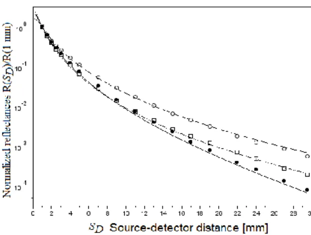
The method of the steady-state (f=0) and the one of the highly modulated source, previously described, (continuous+sinusoïd with high f) could have different efficiencies to make a fitting with the use of the usual equation (1). Indeed, the comparizon between the semi-infinte solution for f=0, Eq. (1), and the Monte Carlo data exhibits closed curves (Figure 3), when the distance range is greater than a few milimiter and smaller than 25-29 mm.

frequency and steady-state. The values of the frequency were set to f=0 and 178MHz. The retrieval algorithm could use up to 18 time-resolved data corresponding to different source-detector distances, SD, ranging from 1mm to 29.5mm (see the symbols in Figure1). To resolve more easily the assessment of the coefficients from the reflectance R according to SD, a transformation of R(SD) to the function ln[SD²R(SD)] is performed, and its slope, computed between 13 and 20 mm, is interpreted as µeff=[3µa(µa+µ's)]1/2. The results of the retrieval, obtained from the two methods, are shown in Table1.

Figure 3. Normalized reflectances R(SD)/R(1 mm) obtained from the Monte Carlo simulation, with a sphere radius rs=35mm, (symbols) and from the equation (1), with C1= 0.118 and C2=0.306, (lines) in the continuous mode (f=0Hz) for 3 set of optical coefficients: round symbols or whole line (0.8mm-1; 0.001mm-1), square symbols or dash-dotted line(1.3mm-1; 0.001mm-1), and black dot symbols or dashed line (1.1mm-1; 0.005mm-1).

Table1 µaf - µsf'

[mm-1_{- mm}-1_]

Method A (C1=0,C2=1)

Retrieved µa Retrieved µs' Method B (C1=0,C2=1)

Retrieved µa Retrieved µs' 0.0225 - 1.45 Continuous 0.0255330 1.3520817 Frequency 178MHz 0.0224038 1.5622084 0.003 - 1.45 Continuous 0.0030737 1.4627461 Frequency 178MHz 0.0035968 1.389302 0.001 - 1.3 Continuous 0.0009952 1.3730456 Frequency 178MHz 0.0027222 1.3231257 0.0075 - 1.25 Continuous 0.0077480 1.2355632 Frequency 178MHz 0.0099701 1.2486994 0.003 - 1.25 Continuous 0.0032991 1.2252735 Frequency 178MHz 0.0036331 1.1107564 0.005 - 1.1 Continuous 0.0049750 1.0633026 Frequency 178MHz 0.0062535 1.0752154 0.001 - 0.8 Continuous 0.0012464 0.7548334 Frequency 178MHz 0.0025876 0.7302197

As expected, the errors with the true values are often greater with the frequency method, especially for the retrieved absorption coefficient. The computations show that the spatially-resolved measurements are often more robust than those obtained by the frequency-resolved mode. However, in high absorbing case (0.0225mm-1; 1.45mm-1), the steady-state method yeilds less accurate retrieved values. The limited number of source-detector distance considered inside a large range (29.5mm) is not adapted when the reflectance decreases rapidly.

To characterize more specifically the spatially-resolved mode by the way of the reflectance imaging, the scale of the continuous procedure was reduced to 0.1mm and extended until 20mm. Those mimic the difference in the use of a CCD camera or of a set of fiber, i.e configurations related respectively to the continuous or the frequency methods. In the Table 2, we observe a slight decrease of the values, but also an improved retrieval in the previously cited case where µa=0.025mm-1.

Table2

0.0225 - 1.45 Continuous SD=0.1mm, 0.1<SD<20mm 0.0226729 1.3708264 0.003 - 1.45 Continuous SD=0.1mm, 0.1<SD<20mm 0.0028329 1.421806 0.0075 - 1.25 Continuous SD=0.1mm, 0.1<SD<20mm 0.0070964 1.2103049 0.003 - 1.25 Continuous SD=0.1mm, 0.1<SD<20mm 0.0032727 1.1703029

From these various results, only those exhibiting a weak absorption parameter can be seen as inadequate. But without absorbtion, the reflectance measurement are going far away from the source position, and the smaller the scale is, the lesser important is the probleme of the curvature. That means to take into account the difference of estimates according to the distance range. For a detection distance used up to 27 mm, i.e largely above the one usually used in hyperspectral imaging4,5, the Fig. 4 shows that the errors occur more rapidly with the decrease of the spherical radius for the case of weak absorption and scattering (µa0 =0.001mm-1 and µ's0 =0.8mm-1) than for the case of high absorption and scattering (µa0 =0.03mm-1 and µ's0 =1.7mm-1).

Figure 4. Normalized optical coefficients, µ's/µ's(1000mm) (line) and µa/µa(1000mm) (dashed), obtained according to the sphere radius rs; (i) and (ii) correspond to the sets (µ's0 =0.8mm-1; µa0=0.001mm-1), and (µ's0 =1.7mm-1; µa0=0.03mm-1), respectively. The source-detector distances, used in the assessment of the optical properties, are extended up to 27 mm.

Furthermore, the frequency modulated mode or the spatially-resolve mode don't use the same kind of mathematical expressions (single intensity or the set phashift and intensity) of the equation (1). So, the optimization algorithms have not the same efficiency. To see the influence of the curved surface on the reference equation (1) in the high frequency domain, another type of comparison is needed.

2.3. Time-resolved methods

The high frequency in a spectral domain corresponds to a weak range in the time domain. So, the assumption of a greater influence of the curvature in the retrieval of optical coefficients for high frequency leads to the idea of a curvature effect in the retrieval with the time-resolved for the close source-detector distances. In order to weigh the efficiency of the retrieval by the resolved expression of the equation (1) (i.e its Fourier transform), another retrieval by a time-resolved method will be made : the Fourier transform is also made on the mathematical solution of the diffusion equation with spherical boundary 13,14,

R

Sph

(θ , f )=

∑

l= 0 ∞

∑

n= 1

P

l

(cos θ) J

l + 1/2

(α

ln

r '

a

)e

2 π

⋅ a

2

(r '⋅ r

s

)

1/2

J

l+ 3 /2

(α

ln

)

2

(

γ

2

− α

ln 2

/a

2

)

[{

α

_ln

a

−

(2 l + 3)l a

α

ln

r

s 2

} J

l+ 3/ 2

(α

ln

r

s

a

)+

l

r

s

J

l+ 5/2

(α

ln

r

s

a

)]

(4) with

r ' = r

s

− 1/ µ

s

' ,a = r

s

+ 4A D

_{, and where J}

time-resolved solution corresponding to a spherical geometry is thus obtained.

From the Monte Carlo simulation, the Figure 5 shows an example of the account of photons according to to the time delay, when the optical coefficients (µ'sth=1.25mm-1; µath=0.0075mm-1) are considered. The time-resolved solutions computed from the Eqs. (1) and (4) are plotted with the fixed set of parameters (µ'sth; µath). Between the peaks and the zero time, the values of the time-resolved related to the Eq. (4) are not considered as available. Despite that, the solution obtained with the spherical boundary, Eq. (4), is from the peak position closer to the data than the one obtained with the semi-infinite geometry, Eq. (1).

Figure 5. Plot of a time-resolved reflectance obtained from the Monte Carlo simulation, with a sphere radius rs=35mm, and from : (a) the Fourier transform of Rsph[asin(SD/rs),f] ; (b) the Fourier transform of R(SD,f).

The same code of Levenberg-Marquardt algorithm was applied for the two retrieval time-resolved methods. The radial source-detector distance was fixed at 11mm. The limit of the time range, needed in order to have a sufficient efficiency, depends on the chosen set of optical coefficients, but we have taken always a maximal time-shift that does not exceed 1.1ns , i.e 20% of the period linked to 178MHz. We are situated on the range corresponding to the weak range in the time domain that was previously mentioned.

Table3 µaf - µsf' [mm-1_{- mm}-1_] Method C (plane) (C1=0,C2=1)

Retrieved µa Retrieved µs' Method D (sphere) (C1=0,C2=1)

Retrieved µa Retrieved µs' 0.0225 - 1.45 Time-resolved 0.0256660 1.4006437 Time-resolved 0.0232297 1.4417957 0.003 - 1.45 Time-resolved 0.0048315 1.3729379 Time-resolved 0.0030057 1.3895091 0.0075 - 1.25 Time-resolved 0.0099419 1.2144671 Time-resolved 0.0073518 1.2695102 0.003 - 1.25 Time-resolved 0.0045985 1.1814145 Time-resolved 0.0029032 1.2252245 The Table 3 depicts the retrieved coefficients. We see a clear difference between the values found in using the equation (1) or (4). The error is more important when the semi-infinite solution (1) is considered. On the contrary, the retrieval of the coefficients is more precise than the Table1 when the sphere geometry is taken into account.

3. CONCLUSION

We have emphasised the idea that a model based on the plane-geometry of a turbid medium is more or less sensitive to its application to curved surfaces depending on the range of time or frequency spectra. The steady-state considered as the case of zero frequency seems to have the ability to support correctly the effect of the boundary curvature. Whatever, the algorithms of the retrieval of tissue optical parameters may be modified by the change of the modelling, as we made here for the time-resolved procedure. Moreover in order to probe the heterogeneity and the multilayered tissues, this

sensitivity to the geometry of the methods of frequency9,15 or of time-resolved16 is needed.

REFERENCE:

[1] E.M.C. Hillman, J. Biomed. Opt. 12 (051402) (2007).

[2] V. V. Tuchin, Tissue optics: light scattering methods and instruments for medical diagnosis, SPIE press Bellingham (2007).

[3] R. Cubeddu, C. D’Andrea, A. Pifferi, P. Taroni, A. Torricelli, G. Valentini, C. Dover, D. Johnson, M. Ruiz-Altisent, and C. Valero, Appl. Opt. 40(4), 538–543 (2001).

[4] J. Qin, and R. Lu, Postharvest Biol. Technol. 49(3), 355–365 (2008). [5] H. Cen and R. Lu, Opt. Express 18(16), 17412-17432 (2010).

[6] C. Abrahamsson, T. Svensson, S. Svanberg, and S. Andersson-Engels, J. Johansson, S. Folestad, Opt. Express 12(17), 4103-4112 (2004).

[7] B. Cletus, R. Künnemeyer, P. Martinsen, A. McGlone, and R. Jordan, J. Biomed. Opt. 14(2), 024041 (2009). [8] S. Fantini, M. A. Franceschini-Fantini, J. S. Maier, S. A. Walker, Opt. Eng. 34, 32–42 (1995).

[9] F. Bevilacqua, A.J. Berger, A.E. Cerussi, D. Jakubowski, and B. J. Tromberg, Appl. Opt. 39, 6498-6507 (2000). [10] F. Vaudelle, J. P. L’Huillier, Influence of the size and skin thickness of apple varieties on the retrieval of internal optical properties using Vis/NIR spectroscopy : a Monte Carlo-based study, submitted to Computers and electronics in Agriculture

[11] A. Kienle and M. S. Patterson, Phys. Med. Biol. 42, 1801–1819 (1997).

[12] T. J. Farrell, M. S. Patterson, and B. C. Wilson, Med. Phys. 19, 879–888 (1992). [13] S. R. Arridge, M. Cope and D.T. Delpy, Phys. Med. Biol. 37, 1531–60 (1992). [14] B.W. Pogue, and M.S. Patterson, Phys. Med. Biol. 39, 1157-1180 (1994).

[15] D. Yudovsky, J. Q. M. Nguyen, and A. J. Durkin, J. Biomed. Opt. 17(10), 107006 (2012)

[16] M. Vanoli, A. Rizzolo, P. E. Zerbini, L. Spinelli, A. Torricelli, Proceedings of the International Conference “Environmentally friendly and safetechnologies for quality of fruit and vegetables” (2009)