HAL Id: hal-01225463
https://hal.archives-ouvertes.fr/hal-01225463
Submitted on 6 Nov 2015
HAL is a multi-disciplinary open access
archive for the deposit and dissemination of
sci-entific research documents, whether they are
pub-lished or not. The documents may come from
teaching and research institutions in France or
abroad, or from public or private research centers.
L’archive ouverte pluridisciplinaire HAL, est
destinée au dépôt et à la diffusion de documents
scientifiques de niveau recherche, publiés ou non,
émanant des établissements d’enseignement et de
recherche français ou étrangers, des laboratoires
publics ou privés.
Performance study of nonlinearities blind correction in
wideband receivers
Raphael Vansebrouck, Chadi Jabbour, Patricia Desgreys, Olivier Jamin, van
Tam Nguyen
To cite this version:
Raphael Vansebrouck, Chadi Jabbour, Patricia Desgreys, Olivier Jamin, van Tam Nguyen.
Perfor-mance study of nonlinearities blind correction in wideband receivers. ICECS, Dec 2014, Marseille,
France. �10.1109/ICECS.2014.7049990�. �hal-01225463�
Performance study of nonlinearities blind correction
in wideband receivers
Raphael Vansebrouck∗†, Chadi Jabbour∗, Patricia Desgreys ∗, Olivier Jamin †, and Van-Tam Nguyen∗‡
∗Institut TELECOM-TELECOM ParisTech, LTCI-CNRS-UMR 5141, France †NXP Semiconductors, Caen, France
‡Department of EECS, University of California at Berkeley, California, 94720, USA
Email: [email protected] Abstract—This paper studies a post-distortion correction
tech-nique applied to a nonlinear receiver. The employed techtech-nique relies on the assumption that the input signal is bandlimited and uses the signal spreading in the free energy band in order to perform the estimation. The study focuses on three points: the input distortion level impact, filter complexity and quantization. A good sizing of these key parameters is mandatory in order to have an optimized CMOS implementation.
I. INTRODUCTION
Nowadays, digital linearization is becoming a very hot topic. With the growth of digital system and shrinking of CMOS technology, digital signal processing is becoming more and more suitable for this issue. Digital techniques like pre-distortions [1] are already widely employed in transmitters for power amplifiers (PA) [2] in order to improve their ef-ficiency [3] and avoid polluting adjacent channels with inter-modulations terms. Digital post-distortion [4] is a recent and attractive approach to fight against nonlinear systems at the receiver side. It can be used to complete a pre-distortion at the transmitter [5], to correct only the receiver part or it can be applied on its own to correct both the transmitter and the receiver nonlinearities.
Several approaches have been proposed in the literature to implement post-distortion corrections. It can be performed after the demodulation similarly to blind channel estimation for equalization. It uses the symbols statistic and tools like high order statistic (HOS). These techniques can be fully blind [6] or aided [7]. For pre-demodulation corrections, one approach consists in adding a low resolution ADC in parallel with an attenuator to avoid the clipping on the strong carriers [8]. A second method uses an interpolation method based on polyphase decomposition to reconstruct the clipped part and thus improve the linearity [9]. Another interesting approach takes advantage of the property of nonlinear systems to spread the spectrum. Actually, if a frequency band at the input of the nonlinear system is free, distortions will appear in this band due to spectrum spreading. An algorithm will seek coefficients for the correction to restrict the output band to the original input band [10][11][12].
This paper provides a system-level framework for the de-sign of blind post-distortion techniques for band-limited de-signal, and the evaluation of their fundamental limits. Indeed, existing papers usually focus on the algorithm design, but do not refer to the limitations induced by realistic usercase and practical implementation. This paper provides a view on the limitations
of these correction systems, and therefore provides an help for this design. Limitations are demonstrated using the algorithm presented in [12]. The aforementioned paper demonstrates the technique for a unique case with a white noise filtered signal of width 0.3 times the sampling frequency, noted fs, and an
input SFDR of 60dB. This paper extends the study, results are shown for several configurations of input signal occupancy and input SFDR. The paper is organized as follows. Section 2 describes the employed blind post-distortion method. Section 3 studies and analyzes, using analytical calculations and system-level simulations, the impact of several parameters such as, distortion level impact, filter complexity and quantization. In the last section, concluding remarks are drawn.
II. PRESENTATION: NONLINEAR CORRECTION SYSTEM STUDIED
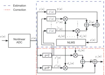
The employed correction system is shown in Fig. 1 [12]. The estimation part is located on the top of the figure and the correction part is located on its bottom. Suppose a weakly nonlinear system, y(n) = Gx(n) + d(n), where G represents the linear gain and d(n) the distortions. If d(n) is sufficiently small then y(n) can be approximated by Gx(n). Therefore if the nonlinear system has been estimated, an estimation of d(n) can be calculated using y(n). Then, the estimated distortion,
ˆ
d(n), is subtracted from y(n). Hence a linearized output yc(n)
can be obtained. We will consider here a polynomial model for the following. To construct the estimated distortion, each nonlinear order is estimated individually and then added. The kth nonlinear component is calculated by y(n) to the power k
(pictured by the block ”p= k” in Fig. 1) and multiply it by the polynomial coefficient αk. The estimation of the coefficients
α is done with the NLMS (Normalized Least Mean Squares) algorithm [13] thanks to the signal spreading property with the band-limited input signal hypothesis. The band-limited assumption on x(n) allows to locate a free-energy frequency band where harmonic distortions and intermodulation terms will fall at the output of the nonlinear system. The NLMS algorithm estimates the coefficients by minimizing the cost function J = E[ke(n)k2], where e(n) is the error between the true (˜y(n)) and the estimated distortion (˜e(n)) in the freeˆ frequency band. This frequency band is recovered by a filter, pictured by f(n) in Fig. 1.
The NLMS is expressed as follows: ˜ αp(n + 1) = ˜αp(n) + µ yp(n)e(n) PP p=1kyp(n)k 2 2 , (1)
where α˜p(n) is the polynomial coefficient of order p, P is
the maximum order considered for the correction and µ is the convergence step. The choice of the NLMS algorithm over the LMS is motivated by a better stability regardless of the input signal statistic and a possible faster convergence compared to the LMS.
Fig. 1. Estimation and correction scheme
III. SYSTEM PERFORMANCE
A. Simulation parameters
As said earlier, the considered system is a nonlinear re-ceiver. In order to limit the calculus length, the nonlinear model is restricted to a third order polynomial model. Nonetheless, following demonstrations can be extended to higher orders.
g(x) = x + 0.003x2
− 0.005x3
. (2)
The convergence step used is set to µ = 0.006. This value, which has been determined in simulations, gives a good compromise between convergence and performance. At the initialization, the estimated polynomial coefficients are set to zero. Due to nonlinear parameters’ estimation, the cost function of the NLMS, J = E[ke(n)k2], which is minimized by the algorithm can include several local minima. This is a common issue with this type of algorithm, this makes the choice of the estimated parameters’ initial value very important in order to have an optimal solution. Nevertheless, since the considered system is weakly nonlinear, the local minima impact is not very critical.
B. Input distortion level impact on the correction efficiency In this subsection, the impact of the input distortion level on the correction performance is studied. As a matter of fact, the correction does not improve the linearity if the input SFDR is smaller than a threshold value. To estimate this point, a normalized two-tone input is used. The considered system can be expressed as: y(n) = Gx(n) + α2x(n) 2 + α3x(n) 3 . (3) d(n) = α2x(n) 2 + α3x(n) 3 , yc(n) = y(n) − ˆd(n), (4)
where d(n) is the distortion term, ˆd(n) the estimated distortion and yc the corrected signal. To reconstruct the estimated
distortion, as said earlier, the following approximation is made: y(n) ≈ Gx(n). ˆ d(n) = 3 X p=2 ˆ αpyp(n) ≈ 3 X p=2 Gpαˆpx(n)p. (5)
Based on the aforementioned approximation, the ideal correc-tion coefficients areαˆ2G
2
= α2 andαˆ3G 3
= α3. The gain is
not of interest in the demonstration, therefore it is fixed to one for convenience. Hence, the corrected output can be developed:
yc=x − 2α 2 2x 3 − (α3 2+ 5α2α3)x 4 − (5α2 2α3+ 3α 2 3)x 5 − (α3 2α3+ 7α2α 2 3)x 6 − (3α2 2α 2 3+ 3α 3 3)x 7 − 3α2α 3 3x 8 − α4 3x 9 . (6)
The considered systems in this study are high performance differential analog front end. As a consequence, the even order harmonics are significantly lower with respect to the odd order harmonics. Hence, the following realistic assumptions are done,|α2| < 1, |α3| < 1 and α3>> α2. We approximate
yc by taking the bigger term in each order:
yc≈ x − 2α 2 2x 3 − 5α2α3x 4 − 3α2 3x 5 − 7α2α 2 3x 6 − 3α2 3x 7 −3α2α 3 3x 8 − α4 3x 9 . (7) At this point, the input and output SFDR can be compared. The term−2α2 2x 3 −3α2 3x 5 −3α3 3x 7 −α4 3x 9
represents the odd order and −5α2α3x 4 − 7α2α 2 3x 6 − 3α2α 3 3x 8
the even order at the correction output. In order to determine the highest distortion, x is linearized to the power p:
xp=X
i
αi(p)sin(2pifi(p)t+ ϕi(p)). (8)
The highest term of distortion for the order p is max(αi(p))
with the condition that fi(p) 6= 0, fi(p) 6= finput1 and fi(p) 6=
finput2. The following table sums up the highest distortion
terms for the considered system for order going from 2 to 9.
p 2 3 4 5
αi(p) 0.25 0.0938 0.1875 0.0977
p 6 7 8 9
αi(p) 0.1465 0.0897 0.1196 0.0807
The input distortion level which gives the same distortion level at the output is:
−0.0807α4 3− (3 × 0.0897)α 3 3− (3 × 0.0977)α 2 3= 0.0938α3. (9) This equation has two complex solutions and one real solution. Since α3must be real, the real solution is kept α3= −0.5583.
This yields in an input SFDR of:
SF DRin= 10 · Log( P s P dist) = −15.31| {z } Ps −(−31.63) | {z } Pdist = 16.32dB, (10)
where Ps and Pdistare, respectively, the input and the
distor-tion power.
Figure 2 shows the output SFDR and the SFDR im-provement with respect to the input SFDR for a two-tone and a Gaussian noise input signals. The square dot is the
0 20 40 60 80 −20 0 20 40 SFDR gain (dB) SFDR in(dB) SFDR gain: Two Tones α 3= −10 α2 0 20 40 60 80−50 0 50 100 150 SFDR out (dB) SFDRout : Two Tones α 3= −10 α2 SFDRout : WGN Theoritical value α 3= −10 α2
Fig. 2. SFDRin effect: correction limit
theoretical value determined in (10). As can be seen, the SFDR improvement is almost equal to zero when SF DRinis
small. The improvement increases significantly once SF DRin
exceeds the theoretical value. Limitation for high SF DRinis
caused by the ADC noise floor. C. Filter Order
In the employed correction, the purpose of the filter is to retrieve distortions from the free frequency band. As a reminder, this filter is pictured by f(n) in the Fig. 1. Ac-tually, if the adjacent bands are not attenuated enough, the correction efficiency is degraded. The NLMS cost function is J = E[|e(n)|2
]. The error signal e(n) is divided into two components eib(n) and eob(n) which are, respectively, the
error signal in the filter passband and stopband. The NLMS cost function becomes then:
J = E[|eib(n) + eob(n)| 2
]. (11) eib(n) and eob(n) are supposed to be independent, therefore
E[eib(n)eob(n)] = 0. J = E[eib(n) 2 + 2eib(n)eob(n) + eob(n) 2 ] = E[eib(n) 2 ] + E[eob(n) 2 ]. (12)
The cost function is then minimized:
min(J) = min(E[eib(n)2] + E[eob(n)2])
= min(E[eib(n) 2
]) + min(E[eob(n) 2
])). (13) The above equation corresponds to two NLMS with the following criteria, min(E[eib(n)2]) and min(E[eob(n)2])).
Leteˆib(n) be the estimated distortion term with the coefficients
retrieved from the first NLMS and ˆeob(n), the estimated
distortion term with the coefficients retrieved from the second NLMS. The signal eˆib(n) has a similar level to the signal
distortion in order to cancel it. Likewise, the signaleˆob(n) has
a similar level to the out-band signal. Nonetheless, eˆob(n) is
an error therefore it adds distortions to the corrected signal. In conclusion, if the out-band signal is not weak enough, the correction level is determined by the difference of level between the in-band signal and the adjacent band. Figure 3 shows the effects of the bandpass size and the filter order on the correction. In this simulation, the employed filters are bandpass FIR filter centered around 0.25 × f s. A margin of
0 100 200 300 400 500 −60 −50 −40 −30 −20 −10 0 10 20 Filter order SFDR gain (dB) 0.02 0.04 0.06 0.08 0.1
Fig. 3. Filter VS Bandpass analysis
0.005 × f s on each side of the bandpass is used. The FIR filters are obtained with the Parks-Mclellan algorithm [14]. The choice of the Parks-Mclellan algorithm is motivated by a significantly lower order for a given ideal filter compared to a windowing method. In Fig. 3, the SF DRgain is shown with
respect to the filter order for different filter bandwidth F BW . Small detection band (BW < 0.1) are chosen to consider a wideband case. The parameter in the figure is bw = F BW
f s .
As can be noticed, the smaller the free bandwidth, the higher the filter order required. For practical implementation, the filter order could be reduced if the selected free bandwidth is larger. For example, a SF DRgain of 15 dB can be achieved with a
filter order less than 100 if bw >0.1 Figure 4 shows the input, the output and the corrected output power spectral density. The input is a filtered white Gaussian noise, which is normalized by its amplitude. The filter bandwidth and the filter order were set, respectively, to0.1 and 100. The correction is about 15 dB between the input and the output SFDR.
D. Quantization
Another important aspect that should be studied is the signal processing quantization or the employed number of bits after mathematical operation. In fact, a high number of bits reduces the quantization noise but on the other hand increases the complexity and consequently the power consumption as well. Therefore, a good compromise should be found in order to optimize the performance. Two analyzes are carried out to determine this compromise value for the filter coefficients and the calculation wordlength.
Let us first analyze the quantization of the filter coefficients.
0 0.1 0.2 0.3 0.4 0.5 −140 −120 −100 −80 −60 −40 Signal PSD Normalized frequency A mplitude (dB) input output Corrected output
10 15 20 25 −15 −10 −5 0 5 10 15 20 25 SFDR gain (dB)
Number of quantizations bits
Calculation Quant with 12−bit ADC Calculation Quant with 14−bit ADC Calculation Quant with 16−bit ADC Filter Coef Quant with 14−bit ADC
Fig. 5. Quantization effect
Fig. 6. Quantization scheme
Figure 5 shows the SFDR with respect to the number of bits in four different scenarios. For the four simulations, the input is a white noise filtered with a lowpass filter with a cut-off frequency of 0.3×fs. The thick bold curve shows the
impact of quantization on the filters for a 14-bit ADC. As can be seen, the SFDR increases with the number of bits nf il. Actually, the filter out of band attenuation decreases
when the coefficients are coded on a lower number of bits. As a consequence, the filtering is less efficient which leads to a SFDR degradation. For the rest of the analysis, the filter coefficients’ number of bits is set to 15 which gives a good compromise between complexity and performance. The coefficients are coded using the canonical signed digit (CSD) representation. This representation reduces the number of non-zero bits in the coefficient coding and consequently reduces the filter complexity.
Let us now study the quantization of the signal process-ing. Figure 6 shows the correction bloc diagram with the quantization at each step of the process. As can be noticed, normalization factors are added when needed to keep the signal in the good range. As a matter of fact, quantization can make the termPPp=0kyp(n)k2
2 become equal to zero which causes
divergence. To overcome this problem, one LSB is added to avoid the divergence. Hence, the NLMS expression becomes:
˜ αp(n + 1) = ˜αp(n) + µ yp(n)e(n) PP p=1kyp(n)k 2 2+ ǫ , (14)
where ǫ = 1LSB. Figure 5 shows as well the impact of the calculation quantization for a 12-bit, 14-bit and 16-bit ADC. As expected, the SFDR increases with the number of bits in the 3 scenarios. However, the maximum achievable SFDR is different in each scenario because as said earlier this
value depends on the ADC quantization noise floor. For the considered 14-bit ADC, 13 bits of quantization gives a good compromise.
IV. CONCLUSION
This paper has studied the operation of a post distortion correction for a wideband receiver. The technique uses the signal spreading in the free energy band in order to perform the estimation. Key parameters required for the implementation such as the distortion level, filter complexity and quantization have been analyzed.
The maximum input distortion level has been determined by the means of analytical calculations and confirmed by simulations. Regarding the filters, it has been shown that there is a tradeoff between their complexity (order and number of bits), the size of the free energy band and the linearity improvement.
REFERENCES
[1] J. Reina-Tosina, M. Allegue-Martinez, M. Madero-Ayora, C. Crespo-Cadenas, and S. Cruces, “Digital predistortion based on a compressed-sensing approach,” in European Microwave Conference (EuMC), Oct 2013, pp. 408–411.
[2] D. Schreurs, M. O’Droma, A. A.Goacher, and M. Gadringer, RF Power Amplifier Behavioral Modeling. Cambridge University Press, 2009. [3] M. Isaksson, D. Wisell, and D. Ronnow, “A comparative analysis of
behavioral models for RF power amplifiers,” IEEE Transactions on Microwave Theory and Techniques, vol. 54, no. 1, pp. 348–359, Jan 2006.
[4] E. Balestrieri, P. Daponte, and S. Rapuano, “A state of the art on ADC error compensation methods,” IEEE Transactions on Instrumentation and Measurement, vol. 54, no. 4, pp. 1388–1394, Aug 2005. [5] A. Ali, O. Hammi, and T. Al-Naffouri, “Compressed Sensing Based
Joint-Compensation of Power Amplifier’s Distortions in OFDMA Cog-nitive Radio Systems,” IEEE Journal on Emerging and Selected Topics in Circuits and Systems, vol. 3, no. 4, pp. 508–520, Dec 2013. [6] N. Kalouptsidis and P. Koukoulas, “Blind identification of
Volterra-Hammerstein systems,” IEEE Transactions on Signal Processing, vol. 53, no. 8, pp. 2777–2787, Aug 2005.
[7] P. Cruz and N. Carvalho, “Multi-carrier wideband nonlinear behavioral modeling for cognitive radio receivers,” in European Microwave Inte-grated Circuits Conference (EuMIC), Oct 2011, pp. 414–417. [8] M. Allen, J. Marttila, and M. Valkama, “Digitally-enhanced wideband
analog-digital interfaces for future cognitive radio devices,” in 8th IEEE International NEWCAS Conference, June 2010, pp. 361–364. [9] ——, “Digital post-processing for reducing A/D converter nonlinear
distortion in wideband radio receivers,” in Conference Record of the Forty-Third Asilomar Conference on Signals, Systems and Computers, Nov 2009, pp. 1111–1114.
[10] L. Duarte, R. Suyama, B. Rivet, R. Attux, J. M. T. Romano, and C. Jutten, “Blind Compensation of Nonlinear Distortions: Application to Source Separation of Post-Nonlinear Mixtures,” IEEE Transactions on Signal Processing, vol. 60, no. 11, pp. 5832–5844, Nov 2012. [11] Y. Ma and Y. Yamao, “Blind nonlinear compensation technique for
RF receiver front-end,” in European Microwave Integrated Circuits Conference (EuMIC), Oct 2013, pp. 556–559.
[12] K. Shi and A. Redfern, “Blind volterra system linearization with applications to post compensation of ADC nonlinearities,” in IEEE International Conference on Acoustics, Speech and Signal Processing (ICASSP), March 2012, pp. 3581–3584.
[13] S. Kalluri and G. Arce, “A general class of nonlinear normalized adaptive filtering algorithms,” Signal Processing, IEEE Transactions on, vol. 47, no. 8, pp. 2262–2272, Aug 1999.
[14] J. McClellan and T. Parks, “A unified approach to the design of optimum fir linear-phase digital filters,” Circuit Theory, IEEE Transactions on, vol. 20, no. 6, pp. 697–701, November 1973.