HAL Id: inria-00438096
https://hal.inria.fr/inria-00438096
Submitted on 2 Dec 2009HAL is a multi-disciplinary open access
archive for the deposit and dissemination of sci-entific research documents, whether they are pub-lished or not. The documents may come from
L’archive ouverte pluridisciplinaire HAL, est destinée au dépôt et à la diffusion de documents scientifiques de niveau recherche, publiés ou non, émanant des établissements d’enseignement et de
A mapping and localization framework for scalable
appearance-based navigation
S. Segvic, A. Remazeilles, A. Diosi, François Chaumette
To cite this version:
S. Segvic, A. Remazeilles, A. Diosi, François Chaumette. A mapping and localization framework for scalable appearance-based navigation. Computer Vision and Image Understanding, Elsevier, 2009, 113 (2), pp.172-187. �inria-00438096�
A mapping and localization framework
for scalable appearance-based navigation ⋆
Siniˇsa ˇ
Segvi´c
a,∗ Anthony Remazeilles
aAlbert Diosi
aFran¸cois Chaumette
aaIRISA/INRIA Rennes, Campus de Beaulieu, 35042 Rennes cedex, France
⋆ This work has been supported by the French national project Predit Mobivip, by the project Robea Bodega, and by the European MC IIF project AViCMaL. ∗ Tel: +385 98 313 325
Email address: [email protected] (Siniˇsa ˇSegvi´c). URL: http://www.zemris.fer.hr/~ssegvic (Siniˇsa ˇSegvi´c).
Abstract
This paper presents a vision framework which enables feature-oriented appearance-based navigation in large outdoor environments containing other moving objects. The framework is based on a hybrid topological–geometrical environment represen-tation, constructed from a learning sequence acquired during a robot motion under human control. At the higher topological layer, the representation contains a graph of key-images such that incident nodes share many natural landmarks. The lower geometrical layer enables to predict the projections of the mapped landmarks onto the current image, in order to be able to start (or resume) their tracking on the fly. The desired navigation functionality is achieved without requiring global geometri-cal consistency of the underlying environment representation. The framework has been experimentally validated in demanding and cluttered outdoor environments, under different imaging conditions. The experiments have been performed on many long sequences acquired from moving cars, as well as in large-scale real-time nav-igation experiments relying exclusively on a single perspective vision sensor. The obtained results confirm the viability of the proposed hybrid approach and indicate interesting directions for future work.
Key words: Visual tracking, point transfer, appearance-based navigation, structure from motion
1 Introduction
Autonomous navigation is an exciting and actively researched application field of computer vision. The design of an autonomous mobile robot requires estab-lishing a close relation between the perceived environment and the commands sent to the low-level controller. This relation is often defined with respect to distinct features which can be extracted from the sensor signal and associated with landmarks from the real world. In order to make the association possible, the robot needs to deal with some kind of an internal representation of the environment. Designing ways to maintain and use this representation is one of the central themes in navigation research [1].
In the model-based approach, the representation is geometric and environment-centred: landmark information is stored explicitly, and expressed in coordi-nates of the common metric frame [2–5]. During navigation, detected features are associated with landmarks in order to localize the robot and to introduce new features. The environment-centric view is intuitively appealing since it decouples the representation from the employed mapping method. However, the required accuracy of the involved estimation process is not easily achieved in practice, which may result in low tolerance to localization and association errors. Additionally, the scalability may be impaired by the complexity of maintaining the global consistency of the model.
In the alternative appearance-based approach, the representation is topolog-ical and sensor-centred: raw sensor readings are organized in a graph where incident nodes correspond to neighbouring locations between which the robot can be controlled easily [6–10]. The navigation goal is planned by finding a
path between the initial and the desired location, while the robot is controlled [11,12] to visit intermediate nodes on the path one by one. The advantages are robust and simple control, as well as outstanding scalability, real-time mapping, and a potential to deal with interconnected environments. On the other hand, the main challenge is to recognize mapped locations in the pres-ence of local sensing disturbances due to occlusions, motion blur, specularities, variable illumination etc.
This paper presents a novel framework for outdoor urban navigation, relying on a single forward-looking perspective vision sensor1
. The framework is based on a hybrid approach [7,17–20], designed to combine prominent properties of the global topological and local geometric environment presentations. We consider separate mapping and navigation procedures as an interesting and not completely solved problem, despite the ongoing work on a unified solution [5]. Unlike many other recent approaches [7,8,20,10], we address perspective vision [9,4] (as illustrated in Figure 1) since it presents attractive opportunities and challenging open problems.
[Fig. 1 about here.]
The appearance of local patches in perspective images is often approximately constant up to scale [21], which presents an opportunity to employ a suitably constrained differential tracker. In comparison with omnidirectional vision, this is of special interest on straight sections of urban roads where forward features are likely to be less influenced by motion blur. On the other hand, the principal challenge in perspective vision based navigation is to successfully handle sharp urban turns, since the lifetime of the tracked features tends to be
short due to fast inter-frame motion. Addressing this challenge while retaining good properties of appearance-based navigation is the central point of this paper.
The paper is organized as follows. Related work in the field of vision-based au-tonomous navigation is discussed in Section 2. Section 3 provides an overview of the proposed navigation framework. The employed vision techniques and algorithms are presented in Section 4, with special emphasis on point transfer. Details of the higher-level procedures used to implement the components of the proposed framework are described in Section 5. Section 6 provides the experimental results including large-scale autonomous navigation of a robotic taxi in a public area. Finally, the discussion with conclusions is provided in Section 7.
2 Related work
In the context of visual appearance-based navigation, nodes of the environ-ment graph are related to key-images acquired from distinctive environenviron-ment locations. Different types of landmark representations have been considered in the literature, from the integral key-image [6,22] and global image descrip-tors [7,23,24], to more conventional point features [25,12,9,10]. The former methods are conceptually simple, but tend to be less tolerant to local sensing disturbances. We focus at the latter feature-oriented approach, where common features are used to navigate between the previous and the next intermediate key-image [12]. Here the effects of local disturbances are limited to loosing contact with particular features which are later safely disregarded by the nav-igation layer. However, in order to ensure seamless operation, contact with
the lost features needs to be re-established as soon as possible. This is es-pecially important with sweeping occlusions which occur so often in urban scenes (e.g. a pedestrian crossing the street in front of the car). Thus, predict-ing approximate locations of currently invisible features (feature prediction) is essential for robust feature-oriented navigation. In our work, feature prediction is also employed for introducing new features along the path.
An appearance-based navigation approach with a rudimental feature predic-tion technique has been described in [26]. The need for feature predicpredic-tion has been alleviated in [9], where new features from the next key-image are intro-duced using wide-baseline matching. A similar approach has been proposed in the context of omnidirectional vision [10]. In this closely related work, fea-ture prediction based on point transfer [27,28] has been employed to recover from tracking failures, but not to introduce new features as well. However, wide-baseline matching is inherently prone to association errors caused by ambiguous landmarks. In our approach, the computationally expensive and not so reliable wide-baseline matching procedure is invoked only once, at the beginning of the navigation. Transitions along the environment graph are per-formed when enough features from the next arc in the environment graph have already been located in the current image.
A model-based point feature-oriented approach described in [4] employs a feature prediction scheme relying on a previously obtained global geometric model. The tracked features are used to update the current estimate of the camera pose, while new features are searched near the projections from their 3D reconstructions. The reported experiments involve successful navigation on the urban paths of over 100 m, for which the model building phase lasts around 1 hour. In comparison, our approach does not require a globally
con-sistent representation of the environment. By posing weaker requirements on the global consistency, we save computation time, likely obtain better local consistencies, and tolerate better difficult situations (such as closing a loop involving a drift with arbitrary magnitude) and occasional correspondence errors.
Notable advances in feature prediction have been achieved in model-based SLAM [29,5,30]. In this approach the 3D locations of all visible features to-gether with the current camera pose are constantly being improved as the navigation proceeds. The location of previously seen but currently non-tracked features can consequently be predicted by simple projection. Nevertheless, current implementations have limitations with respect to the total number of tracked points. Therefore, a prior learning step still seems a reasonable option in realistic navigation tasks. In comparison, our approach has practically no scaling problems whatsoever: experiments with 15000 landmarks have been performed without any performance degradation.
An account of advantages of hybrid representation in exploratory navigation has been presented in [17]. The global consistency has been addressed in a slightly different manner in [19], where loop closure has been postponed by using manifold maps (which are related to topological representation), and eventually enforced by active data association through robot rendezvous. A related approach has been employed in [18] in order to obtain photorealistic walkthroughs starting from a sparse set of stereoscopic images. However, these approaches do not address details specific to outdoor navigation with a single perspective camera.
be found in [7], where the appearance-based indoor navigation is performed using omnidirectional images. The indoor environment is heavily structured which enables using different descriptions in different parts of the environ-ment. Along a corridor, the system only has to track the parallel longitudinal edges, in order to maintain itself far from the walls. Turning around corners is considered more difficult and is more precisely controlled by tracking features acquired during a previous learning step. In comparison with our work, the au-thors do not address building the hierarchical representation in an automatic fashion and predicting the positions of currently invisible features.
3 Overview of the proposed navigation framework
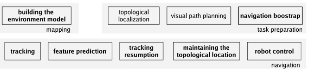
The proposed framework for appearance-based navigation is a long-term re-search goal at our laboratory [31,13,16,32]. As illustrated in Figure 2, the framework operates in three distinct phases which are going to be introduced in the following subsections. But before that, we first briefly state the assump-tions and constraints used to conceive the framework.
[Fig. 2 about here.]
3.1 Assumptions
We consider an autonomous car-like robot within a previously mapped public urban environment. The robot employs a perspective camera with fixed and known intrinsic parameters as the only sensing modality. We assume paved paths with reasonable longitudinal and lateral inclinations. Thus, the appear-ance of visible landmarks is expected to change mostly with respect to scale,
since the camera has a moderate field of view. This consequence is employed to achieve reliable tracking of suitable square patches [33] (or point features) over extended image sequences.
The presented framework is concerned only with goal-directed behaviour, while obstacle avoidance will be considered in the future work. Thus, in the navigation experiments we assume that other moving objects will adopt collision-free trajectories, while a human supervisor is responsible for handling the emergency stop button. The devised control procedure achieves a qualita-tive path following behaviour, since the learned path is not tracked precisely in general. It is therefore suitable to prefer the center of the free space during the acquisition of the learning sequence.
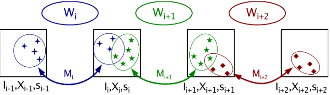
3.2 The mapping phase
The hybrid topological–geometrical environment representation is created from a given learning sequence acquired during a robot motion under a human con-trol. Global topological representation is automatically formed by selecting key-images from the learning sequence and organizing them within an ad-jacency graph. A distinct local geometrical representation is constructed for each neighbouring pair of key-images from extracted point correspondences. Structure of the hybrid representation is illustrated in Figure 3. Key-images Ii correspond to nodes of the environment graph. The associative maps Xi
store 2D coordinates of point features qij located in Ii, and indexes them by
unique feature identifiers. When a common physical structure is detected in two images Ii1 and Ii2, the corresponding points in Xi1 and Xi2 are denoted
by a common identifier. For each arc k, the array of identifiers Mk denotes the
corresponding features in the two incident nodes. Arcs are further annotated with two-view geometries Wk, constructed from the correspondences defined
by Mk. The elements of Wkinclude motion parameters Rkand tk(normalized
to the unit distance), as well as the 3D reconstructions Qkj of the
correspond-ing features indexed by the respective identifiers. The two-view geometries Wk
are deliberately set to unit scale, since contradicting scale sequences may be obtained along the graph cycles.
[Fig. 3 about here.]
In the presented implementation, we consider only linear and circular graphs (cf. Figure 3). The same indexing is used both for nodes and arcs, by em-ploying the convention that arc i connects nodes i − 1 and i. If the graph is circular, arc 0 connects the last node n − 1 with the node 0. Thus, the cur-rent geometric model Wi+1 corresponds to key-images Ii and Ii+1. Similarly,
model Wi corresponds to key-images Ii−1 and Ii, while Wi+2 corresponds to
Ii+1 and Ii+2. The scale si denotes the relative scale between the geometries
Wi and Wi+1. More details about the concrete procedures used to implement
the described mapping functionality are provided in 5.1.
3.3 The task preparation phase
The task preparation phase is performed after the navigation task has been presented to the navigation system. In general, it consists of determining topo-logical locations of the initial and desired robot positions, visual path planning and bootstrapping the navigation phase [32]. However, the focus of this work
is on mapping and real-time navigation issues so that the required topological locations are simply provided by the user. Furthermore, here we only con-sider linear and circular topological representations which obviates the need for path planning2.
The navigation phase is bootstrapped by locating mapped features within the image acquired from the initial robot location. In order to achieve that, the initial image needs to be related to the local frame Wi+1 at the initial
topological location. Consequently, the two-view geometries towards the two incident key-images Ii and Ii+1 are recovered by wide-baseline matching. This
allows to predict the positions of the mapped features within the initial image using the procedure described in 5.2.1 and consequently start the navigation.
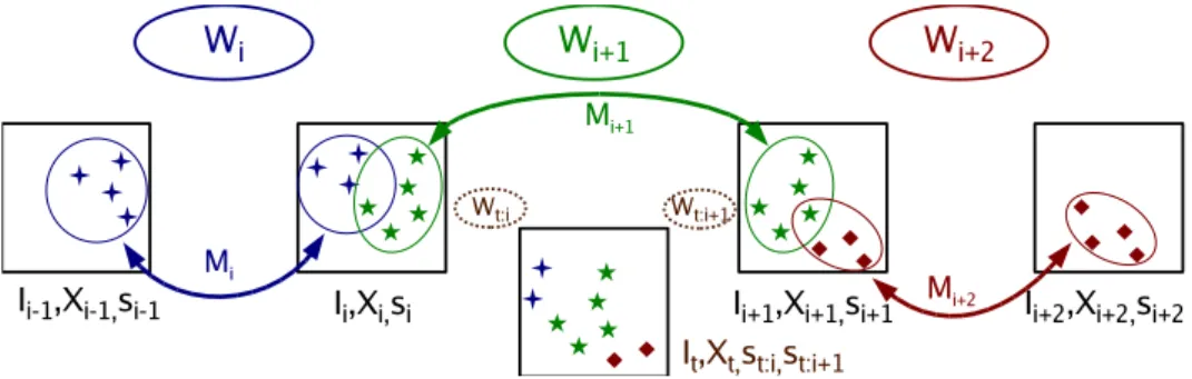
3.4 The navigation phase
The navigation phase involves a visual servoing processing loop [35], in which point features from images acquired in real-time and their correspondences from the key-images are used to control the robot. Thus, two distinct kinds of localization are required: (i) explicit topological localization, and (ii) implicit fine-level localization through the locations of the tracked features. The topo-logical location corresponds to the actual arc of the environment graph which determines the two key-images used in visual servoing (cf. Figure 4). Ideally, the actual arc should denote the key-images having most content in common with the current image. This is usually well defined in practice since the mo-tion of a robotic car is constrained by the traffic infrastructure. Maintaining
2 Refer to [34,32] for a more involved treating of these issues based on content based
an accurate topological location is important because that determines which landmarks are considered for tracking in the current image, and eventually employed to control the robot.
[Fig. 4 about here.]
When a new image is acquired, previously visible features are tracked (cf. 4.2), while their positions are used to perform other tasks within the process-ing loop (cf. Figure 2). As the robot navigates, it eventually gets close to the next key-image along the desired path. The topological location is then smoothly changed towards the next arc and the associated geometric sub-world (cf. 5.2.2). The smooth transitions are possible since we track not only the features from the actual arc, but also the features from the neighbouring two arcs (cf. Figure 4). During the motion, the tracking of some features fails due to contact with the image border or local sensing disturbances. Feature prediction allows to deal with this problem and resume the feature tracking on the fly while minimizing the chances for correspondence errors (cf. 5.2.1). Fi-nally, the vectors between the actual positions of the tracked points and their correspondences in the next key-image are employed to control the motion of the vehicle using an adequate visual servoing [35] procedure (cf. 6.3).
The devised hierarchical environment representation strives to keep the best from topological and geometric approaches. The global topological layer en-sures scalability, fast mapping and robust control. The local geometric models support feature prediction which facilitates dealing with large inter-frame mo-tions and local disturbances in the input image stream. We strive to obtain the best predictions possible, and therefore favour local over global consistency by relaxing the requirement for a globally consistent environment model. The
procedures dealing with real-time localization issues are described in more detail in 5.2.
4 Vision techniques and algorithms
This section presents the lower-level building blocks of the proposed frame-work. The presented techniques and algorithms are wide-baseline matching, point feature tracking, camera calibration, point transfer and evaluation of a two-view geometry.
4.1 Wide-baseline matching of point features
In wide-baseline matching the correspondences are found without any assump-tions about the relative pose of the two input images. An important capabil-ity of the matching algorithm is therefore to recognize the two image patches projected from the same landmark even when they are related by a complex transformation including scale, rotation, and affine or photometric warps. In the considered application, images are taken from a moving car which implies that the predominant appearance distortion is along the scale axis.
The implemented procedure is based on L2 matching of SIFT descriptors [36]. The key-points for calculating the descriptors are extracted using the maxima of the difference of Gaussians [36], multi-scale Harris corners [37], and maximally stable extremal regions (MSER) [38]. We employed suitably wrapped binary implementations of the three key-point extraction algorithms kindly provided by the respective authors3. Three sets of correspondences 3 Executables for the three key-point extraction algorithms are accessible from:
are obtained by matching descriptors calculated at key-points provided by the three extraction algorithms. The correspondences are fused by allowing only one key-point in the radius of a few pixels. Combining the three algorithms is advantageous, since they extract different kinds of features and therefore often complement each other.
The employed algorithm for estimating the epipolar geometry (cf. 4.4) proved quite sensitive to the accuracy of the correspondences. The matching proce-dure is therefore configured in order to minimize inaccuracies. The ambiguities in urban scenes are addressed by the simple rule, to keep only those features for which the distance in the second-best match is less than 60% of the distance in the best match [36].
4.2 Point feature tracking
Two main approaches for conceiving a point feature tracker are iterative first-order differential approximation [33,39], and matching of light-weight point features using a proximity gate [40]. In both approaches, a straightforward so-lution based on integrating the inter-frame motion is viable only for short-term operation, due to incontrollable growth of the accumulated drift. It is there-fore necessary either to adapt the higher-level task to work only with short feature tracks [40], if applicable, or to devise a monitoring scheme for correct-ing the drift [33]. Drift correction is particularly suitable in our context, since
Difference of Gaussians: http://www.cs.ubc.ca/∼lowe/keypoints/
Multiscale Harris: http://lear.inrialpes.fr/people/dorko/downloads.html MSER: http://www.robots.ox.ac.uk/∼vgg/research/affine/detectors.html
the short-lived features are less adequate for appearance-based navigation. The drift is usually corrected by aligning (or warping) the current appearance of the feature with a previously stored template image or reference. The desired alignment is performed by minimizing the norm of the error image, which is obtained by subtracting the current feature from the reference [41]. Shi and Tomasi [33] have proposed a warp with 6 free parameters corresponding to a 2D affine transform, which can account for deformations of planar features in most situations of practical importance. An extension of their work has been proposed in [39], where the warp additionally compensated for affine photometric deformations of the grey level value in the image.
Our best results have been achieved by a custom multi-scale differential tracker [21] derived from the implementation maintained by Stan Birchfield at the Clemson university4. The employed warp consists of translation, isotropic
scaling and affine contrast compensation. The tracker typically manages to handle disparities of more than 10 pixels. More implementation details have been provided in [21].
4.3 Camera calibration
In real time robotic applications of computer vision, the processing is often performed on images acquired by a particular carefully selected camera. Cam-era calibration is therefore a good opportunity to decrease the error in the in-put data (typically, the coordinates of the extracted features), and at the same time avoid projective ambiguities. The employed calibration procedure [42]
termines 5 parameters of a linear model organized in a matrix K, and 2 pairs of parameters modelling radial distortion (kud
1 , k2ud) and correction (k1du, kdu2 )
[43]. Both directions of the radial model are needed since the tracked points need to be corrected before being given to stereo reconstruction, while the predictions need to be distorted before a new feature is actually searched for in the current image.
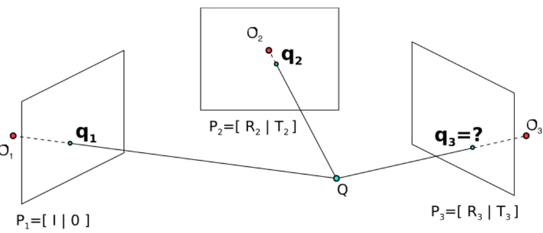
4.4 Decomposed point transfer in the calibrated context
Point transfer [27,28] refers to projecting a point visible in two views of the same scene onto a new view, by using other correspondences between the three views. The technique allows to predict the current position of a fea-ture matched between the two neighbouring key-images, provided that the corresponding three-view geometry [28] has been previously recovered.
There are many ways to compute the three-view geometry, with different as-sumptions and performance requirements. The “gold standard” method de-scribed in [28] involves bundle adjustment with respect to the reprojection error in all views, which may be too expensive in a real time implementation. Additionally, the standard method does not use pairwise correspondences, but only the points visible in all three images. This is a remarkable loss of informa-tion since in our experiments pairwise correspondences were more than twice as numerous than the three-way correspondences. Finally, during navigation, the estimation of the three-view geometry is performed many times for each neighbouring pair of key-images. Thus it is advantageous to precompute two-view geometries between neighbouring key-images and store them as a prop-erty of the incident arc. An efficient formulation of such decomposed solution
has been proposed and evaluated by Lourakis and Argyros in the uncalibrated (projective) context [44]. Very good experimental results have been reported although the approach is suboptimal. The same idea has been employed in this paper, but within the calibrated context (cf. Figure 5). The desired three-view geometry is obtained by combining a precomputed two-three-view geometry between the two key-images with a two-view geometry between the current image and one of the two key-images.
[Fig. 5 about here.]
The two-view geometries are recovered using the essential matrix estimated by the random sampling scheme MLESAC [45], using the recent five point algo-rithm [46] as the generator of motion hypotheses. The employed implementa-tion has been provided within the libraryVW345 maintained at the University of Oxford. The decomposition of the essential matrix into motion components is performed next, followed by the triangulation of 3D points [28]. Before pro-ceeding, the two two-view geometries need to be expressed in a common frame. It is advantageous to stay in calibrated context, since the adjustment of two metric frames involves estimation of only one parameter (scale), while in the projective context the ambiguity has 4 degrees of freedom [44]. The scale fac-tor between two metric frames is estimated by requiring that all points visible in both frames have the same depth. In practice, different points vote for dif-ferent scale factors due to noise. A robust result is in the end obtained as the median of all individual factors.
4.5 Evaluation of a two-view geometry
It is important to be able to tell whether an estimation of a two-view geometry has succeeded or not, especially when the result is used for navigation. We noticed that the root-mean-square reprojection residual correlates well with the quality of the recovered geometry, except at occasions when the calculation involves a small number of correspondences. A theoretical explanation for these exceptions has been found, and a better measure is proposed, based on a conservative estimation of the variance of the reprojection error.
Assume that the two-view geometry has been estimated by random sampling, and let the random variables Dix and Diy be assigned to the two reprojection
error components of the i-th inlier point used in the estimation. We assume that these 2n variables are independent, and that they have a common normal distribution with zero mean [28]:
Dix, Diy ∼ N (0, ˆσ2), i = 1, 2, . . . , n. (1)
We wish to estimate a conservative upper bound σ2
p of the common pixel error
variance ˆσ2
, with a tolerated probability p of making an error:
σp = arg minσ P (ˆσ > σ) < p. (2)
We notice that P (ˆσ > σp) = p, and introduce an auxiliary random variable Z
as follows: Z =X i (D2 ix+ D 2 iy)/ˆσ 2 . (3)
Under the assumption (1), Z is distributed as χ2 with 2n degrees of freedom
(2n because the mean of the variables is assumed, and not estimated), so that: P (Z < z) = Fχ2(z; 2n), (4)
where Fχ2(z; 2n) corresponds to a cumulative probability function. Conse-quently, by substituting (3) and z =Pi(D2ix+ D
2 iy)/σ 2 p into (4), we obtain: P (ˆσ2 > σ2 p) = Fχ2( X i (D2 ix+ D 2 iy)/σ 2 p; 2n). (5)
Finally, by combining (5) and (2), an expression for σ2
p is derived in terms
of the count of the observed points n, and the parameter p describing the accepted risk: σp2 = P i(D2ix+ D 2 iy) F−1 χ2 (p; 2n) . (6)
The inverse of the cumulative probability function can be determined using a precalculated table for a feasible range of n, and a chosen p, e.g, p = 0.05. Note that for a large n, the denominator in (6) tends towards 2n, leading to the usual root-mean-square residual. The presented idea of penalizing geome-tries recovered with small numbers of points should be applicable even in the presence of outliers. In this case the denominator in (6) could be determined using a robust estimator such as median absolute deviation.
5 Implementation details of the proposed framework
This section describes implementation details of the high-level vision compo-nents of the proposed framework. The mapping component defines the be-haviour of the system within the mapping phase: it creates the environment representation from a learning sequence, as introduced in 3.2. The behaviour in the navigation phase is implemented by the localization and control com-ponents. The localization component tracks the mapped features, employs them to locate new features and maintains the correct topological location, as introduced in 3.4. The output of the localization component is a set of
vec-tors connecting the current feature positions and their correspondences in the next key-image. These vectors are provided to the control component which is briefly described along the navigation experiments in 6.3.
5.1 The mapping component
Many maps can be constructed for the same learning sequence, depending on the selected set of key-images and on the technique for extracting corre-spondences. Quantitatively, a particular arc of the map can be evaluated by an estimate of the reprojection error [28] σp(Wi) from (6), and the number of
correspondences |Mi|. The two parameters are related to accuracy of the point
transfer, and robustness to local sensing disturbances. There is a trade-off in interpreting the criterion |Mi|, since more points usually means better
robust-ness but lower execution speed. Different maps of the same environment can be evaluated by the total count of arcs in the graph |{Mi}|, and by the
param-eters of the individual arcs σp(Wi) and |Mi|. It is usually favourable to have
less arcs since, for a given deviation, that ensures a smaller difference in lines of sight between the relevant key-images and the images acquired during nav-igation. This is important since the ability to deviate from the reference path enables the robot to tolerate control errors and to avoid detected obstacles.
Two different options were considered to address the issues above and achieve automatic mapping of the environment. The alternatives are detailed and discussed in the following text.
5.1.1 Mapping by matching
The first considered mapping option is wide-baseline matching of images from the learning sequence. A simple key-image selection technique is employed, in which initially each 30th frame is selected. If for a certain index i the count of obtained matches |Mi| is too small or the reprojection error σp(Wi) is too
large, a new key-image is introduced between the two considered ones, and the procedure is recursively repeated.
As presented in 4.1, a heterogeneous matching algorithm is employed, pro-viding features which are not necessarily compatible with the tracker. For instance, a valuable SIFT feature calculated in the centre of a 30×30 pixels distinct blob might not be trackable with a fixed feature window of 15×15 pix-els. Such inadequacies of the features proposed by the matcher are detected immediately after the matching, by trying to track each feature at the matched location in the other image. Inadequate features are used only for recovery of the two-view geometry, and disregarded within the localization component. Unfortunately, the above matching procedure does not always succeed to re-cover a two-view geometry with an acceptable level of accuracy. In particu-lar, the accuracy is not always proportional to the success of the matching algorithm. This is because, as the physical distance between two successive camera poses decreases, the count of obtained correspondences increases, to-gether with the difficulty of the reconstruction problem due to a small baseline [46]. Thus it can happen that an accurate solution in terms of σp(Wi) can not
be found e.g. for images n and n + 5 of the learning sequence, but a per-fectly valid solution can be found between n and n + 14, although with less correspondences.
5.1.2 Mapping by tracking
In this mapping option, the tracker is used to find very stable point features in a given subrange of the learning sequence. The tracker is initialized with all Harris corners in the initial frame of the subrange6
. The features are tracked until the reconstruction error between the first and the current frame of the subrange rises above a predefined threshold σp. At this moment the current
frame is discarded, while the previous frame is registered as the new key-image in the environment graph, and the whole procedure is repeated from there. To ensure a minimum number of features within an arc of the graph, a new node is forced when the absolute number of tracked points falls below n. Bad tracks are identified by a threshold R on the RMS residual between the current feature and the reference appearance [33,21]. Typically, the following values were used: σp = 4, n = 50, R = 6.
A similar mapping procedure has been used in [9], but without monitoring the reconstruction error. The proposed mapping is similar to the recent visual odometry technique [40], except that we employ larger feature windows and more involved tracking (cf. 4.2) in order to achieve more distinctive features and longer feature lifetimes. The obtained key-images are related to key-frames in structure and motion estimation [47,4] since both provide a solution to the problem of increasing noise in tracked feature positions. However, the purpose of the two is different, since our key-images need to be as far apart as possible
6 Although the two-view geometry estimation tends to be more accurate when the
correspondences are distributed evenly, we do not try to enforce that. This is because real environments tend to be unevenly rich in information content. Enforcing a better spatial arrangement by favouring the correspondences in the sky, on the pavement, or on the blank wall would likely deteriorate the results.
in order to be more suitable for appearance-based navigation.
Generally, the tracking approach provided substantially better results than the approach based on matching, both in terms of reprojection error and the count of mapped features. In the overwhelming majority of experiments the accuracy was satisfactory even for very small baselines. This should be regarded as no surprise, since more information is used to achieve the same goal. However, exceptions to the above occur when there are discontinuities in the learning sequence caused by a large moving object, or a “frame gap” due to preemption of the acquisition process. In the presented scheme, such events are reflected by a general tracking failure in the second frame of a new subrange. In principle, both of these problems can be avoided by carefully preparing the acquisition of the learning sequence, since the main goal of the system is to achieve robustness during the navigation phase. Nevertheless, we try to solve these problems automatically. A recovery is attempted by matching the last key-image with the current image in order to connect the disjoint parts of the graph. This is especially convenient when mapping is performed online, from a manually controlled robotic car.
Wide-baseline matching is also useful for connecting a cycle in the environment graph, which is applicable if the learning sequence has been acquired along a closed physical path such that the initial and final positions are nearly the same. After the learning sequence acquisition is over, the first and the last key-image are subjected to matching: a circular graph is created on success, and a simple linear graph otherwise. In the case of a monolithic geometric model, the above loop closing process would need to be followed by a sophisticated map correction procedure, in order to try to correct the accumulated error [48,49]. Due to topological representation at the top-level, this operation in
our framework proceeds reliably and smoothly, without any restrictions related to execution speed or the extent of correction. The only consequence is that one needs to renounce to absolute scale factors of the individual geometries, since the sequence of scales along the arcs of a cycle may not be consistent in general. However this can be solved by storing the relative scale of each pair of neighbouring edges within the common node, as described in 3.2.
5.2 The localization component
The localization component is responsible for all procedures from the nav-igation phase (cf. 3.4) except the robot control. The tracking procedure is decoupled from the rest of the framework and is as such described separately in 4.2. Therefore, here we describe in more detail feature prediction and track-ing resumption, as well as maintaintrack-ing the correct topological location. Note that the navigation is bootstraped from the local geometries recovered from correspondences obtained by wide-baseline matching, as described in 3.3.
5.2.1 Feature prediction and tracking resumption
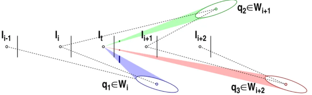
The point features which are tracked in the current image It are employed to
estimate the two-view geometries Wt:i(Ii, It) and Wt:i+1(Ii+1, It) towards the
two key-images incident to the actual arc (cf. Figure 4). As detailed in 4.4, the three-view geometry (It, Ii, Ii+1) is recovered by adjusting the precomputed
two-view geometry Wi+1 towards the more accurate of Wt:i and Wt:i+1.
Simi-larly, the geometry (It, Ii+1, Ii+2) is recovered from Wi+2and Wt:i+1, while the
geometry (It, Ii−1, Ii) is recovered from Wi and Wt:i. Current image locations
(It, Ii, Ii+1). Landmarks from the previous arc i and the next arc i + 2 are
transferred by geometries (It, Ii−1, Ii) and (It, Ii+1, Ii+2), respectively.
The obtained predictions are employed only if the estimated reprojection error σpfrom (6) of the selected current geometry is less than a predefined threshold.
The predictions are refined by minimizing the residual between the warped current feature and the reference appearance, as in the tracker. The initial scale of the feature [21] is set by dividing the distance of the reconstructed 3D point towards the current pose, with the distance of the same 3D point towards the viewpoint of the image used to initialize the reference. As in tracking, the result is accepted if the procedure converges near the predicted location and scale, with an acceptable residual.
The above concept substantially improves the application field of the point tracker. However, a special care must be taken in order not to introduce an association error, by resuming a similar feature in the neighbourhood. As illustrated in Figure 6, the reprojection uncertainty is greatest for the features from the previous arc, which tend to be the nearest, and smallest for the farthest points from the next arc. However, Figure 6 does not take into account the risk of making an association error which is the greatest for the features from the next arc, which are likely to be tracked farthest in the future. A prudent strategy is therefore taken, in which the tracking of the features from the next arc is resumed only if the current pose is closer to the next node. If we introduce st:i+1 as the recovered scale of Wt:i+1 with respect to Wi+1
(cf. Figure 4), then the above criterion can be concisely written as:
st:i+1· ktt:i+1k/ktik < 0.5 . (7)
the connection with the features from the previous node:
st:i· ktt:ik/ktik < 0.3 . (8)
[Fig. 6 about here.]
Other than for introducing new features, the above procedure is also employed to check the consistency of the tracked features, which occasionally “jump” to the occluding foreground. Thus, following the sanity check on the employed two-view geometry, the tracking of a feature is discontinued if the tracked position becomes too distant from the prediction.
5.2.2 Maintaining the topological location
Maintaining a correct topological location is critical in the proposed frame-work since both feature prediction and robot control depend on its accuracy. An incorrect topological location leads to suboptimal introduction of new fea-tures, which may be followed by by a failure due to insufficient features for calculating Wt:i and Wt:i+1 (cf. Figure 4). This is especially the case in sharp
turns where many landmarks from the neighbouring geometries project out-side of the current image borders.
After experimenting with different approaches, best results have been obtained using a straightforward geometric criterion. Following this criterion, a forward transition is taken whenever the camera pose in the actual frame Wi+1 comes
in front of the farther camera Ii+1. This can be expressed as:
h−Ri+1⊤· ti+1, tt:i+1i < 0 (9)
Wt:i+1, which is geometrically closer to the hypothesized transition, as shown
in Figure 7. As in 5.2.1, the transition is cancelled if the estimated reprojection error σpfrom (6) of the employed current geometry is not less than a predefined
threshold. Backward transitions are analogously defined in order to support reverse motion of the robot.
[Fig. 7 about here.]
After each change of the topological location, the reference appearances are redefined for all relevant features in order to achieve better tracking. For for-ward transitions, references for the features from the actual geometry Wi+1are
taken from Ii+1, while the references for the features from Wi+2are taken from
Ii+2 (cf. Figure 4). The tracking of previously tracked points from geometries
Wi+1 and Wi+2 is instantly resumed using their previous positions and new
references, while the features from Wi are discontinued.
6 Experimental results
The experiments have been carried out on sequences acquired by a camera mounted on an electric car-like robot named Cycab, and in real-time during autonomous navigation. The presented experiments consider realistic physical paths for which no common landmarks are visible from the initial and the desired position. The experiments are also illustrated in the videos which can be accessed from:
• http://www.irisa.fr/lagadic/video/CycabNavigation.mov
• http://www.zemris.fer.hr/∼ssegvic/pubs/diosi07iros 0581 VI i.mp4
6.1 Mapping experiments
Two groups of mapping experiments will be presented. In the first group, the two mapping approaches are applied to the same learning sequence. The sensitivity of the better approach to the choice of parameters is investigated in the second group.
6.1.1 Comparison of the two mapping approaches
The two mapping approaches described in 5.1 have been experimentally com-pared on the learning sequence ifsic5. The sequence contains 1900 frames acquired along a physical path of about 150 m, corresponding to the reverse of the path shown in Figure 1. For illustration, the set of key-images obtained by the tracking approach is presented in Figure 8.
[Fig. 8 about here.]
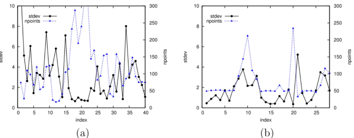
The comparison was performed in terms of parameters of the obtained geo-metric models which were introduced in 5.1. These parameters were: (i) the number of point features |Mi| (more is better), (ii) the reprojection error
σp(Wi) (less is better), and (iii) the frame distance (related to |{Mi}|, larger
is better). The obtained values for the first two parameters are summarized in Figure 9.
[Fig. 9 about here.]
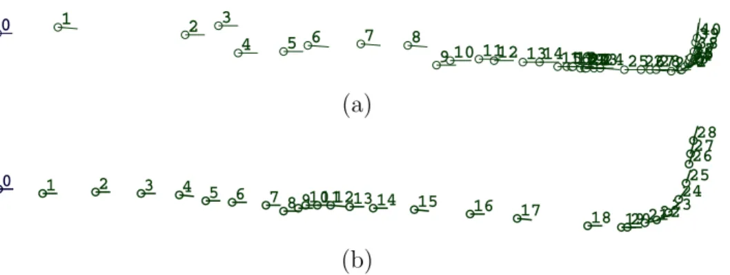
Qualitative illustration of the third parameter (inter-frame distance) is shown in Figure 10 as the two sequences of recovered camera poses corresponding to the nodes of the environment graph (common global scale is enforced for
vi-sualization purposes). The figure shows that the matching approach produced more key-images (40 vs. 30), while their spatial arrangement is less coherent than what can be observed for the tracking approach. Thus, the figures show that two of the relevant parameters (frame distance and reprojection error) are considerably better when the mapping is performed by the tracking approach. Similar results have been obtained for other sequences as well.
Figure 10 suggests that the tracking approach produces predictable results by adapting the density of key-images to the inherent difficulty of the scene. The matching approach on the other hand at times produces a large number of correspondences, but their quality is sometimes insufficient for recovering a usable two-view geometry. The dense nodes 7-14 in Figure 10(b) correspond to the first difficult moment of the learning path (cf. Figure 8, middle row and Figure 1, reverse direction): approaching the traverse building and pass-ing underneath it. Nodes 20 to 25 correspond to the sharp left turn, while passing very close to the building which can be seen in Figure 8. The difficult conditions persisted after the turn due to large featureless bushes and a re-flecting glass surface: this is reflected in dense nodes 26-28, cf. Figure 10(b). Figure 9(b) shows that the number of features in arc 20 is exceptionally high, while the incident nodes 19 and 20 are very close. The anomaly is due to a large frame gap causing most feature tracks to terminate instantly. Here the tracking approach had been automatically aided by wide-baseline matching, which succeeded to relate the key-image 19 and its immediate successor which consequently became key-image 20. The error peak in arc 21 is caused by another gap which had been successfully bridged by the tracker alone.
To summarize the above experiments, the tracking approach to mapping is a reasonable default option. However, in exceptional situations such as when some frames in the input sequence are missing or after a total occlusion by a moving object, better results are obtained by the described combination with matching.
6.1.2 Sensitivity of the mapper to the choice of parameters
In the following text, a circular sequence will denote a sequence acquired along a closed physical path. In order to acquire such sequence, the initial and final robot coordinates need to be similar or the same, while the interval of attained viewing directions needs to be [0, 2πi. Note that here we consider only car-like robots which are not capable to perform pure rotational motions.
Circular sequences are especially suitable for testing the mapping alternatives since they provide an intuitive notion about the achieved overall accuracy. The sensitivity of the mapping algorithm to the three main parameters was tested on the circular sequence loop-clouds taken along a path of approximately 50 m. The resulting poses are plotted in Figure 11 for 4 different triplets of mapping parameters described in 5.1.2: (i) minimum count of features n, (ii) maximum reprojection error σp from (6), and (iii) the maximum RMS residual
R used to detect unreliable feature tracks. [Fig. 11 about here.]
Reasonable and usable representations were obtained (cf. Figure 11) despite the smooth planar surfaces and vegetation which are visible in Figure 12. The presence of node 0’ indicates that the cycle at the topological level has been
successfully closed by wide-baseline matching. Ideally, nodes 0’ and 0 should be very close; the extent of the distance indicates a large magnitude of the accumulated drift in the result with n=25. The relation between the two nodes in the results with n=50 and n=100 suggest that the distance between the corresponding locations is around 1.5 m.
[Fig. 12 about here.]
The experiments show that there is a direct coupling between the number of arcs |{Mi}|, and the number of features in each arc |Mi|. Thus, it is beneficial
to seek the smallest |{Mi}| ensuring acceptable values for σp(Wi) and |Mi|.
The requirement that neighbouring triplets of images need to contain common features did not cause problems in practice: the accuracy of the two-view geometries σp(Wi) was the main limiting factor for the mapping success.
In some cases, a more precise overall geometric picture might have been ob-tained by applying a global optimization post-processing step. This has been omitted since in our context, global consistency brings no immediate benefits (and poses scalability problems). Enforcing the global consistency is especially fragile for forward motion which occurs predominantly in the case of the car-like robots. In this context, more than half of the correspondences are not shared between neighbouring geometries, and the ones that are shared are more likely to contain association errors due to a larger change in appearance. The last map in Figure 11 (bottom-right) was deliberately constructed us-ing suboptimal parameters, to show that our mappus-ing approach worked even when enforcing global consistency would likely have been difficult.
6.2 Localization experiments
In the following paragraphs, we shall focus on the individual aspects of the localization component. These aspects are robustness to moving objects, ro-bustness to different imaging conditions, quantitative success in recognizing mapped features and the capability to traverse topological cycles.
6.2.1 Robustness to moving objects
In this group of localization experiments, the capability of the localization component to correctly resume temporary occluded and previously unseen features have been tested. Illustrative feature tracking results are presented in Figure 13. The figure shows a situation in which six features have been wiped out by a moving pedestrian, and subsequently resumed without errors. The employed map has been illustrated in Figures 9(a) and 10(a), and discussed in the accompanying text.
[Fig. 13 about here.]
The figure shows that the point transfer is accurate, since the projections of the occluded features have been correctly predicted. These features have been designated with crosses, since the predictions have been rejected due to a differing appearance. In the case of feature 146 in frame 743, the tracker “zoomed out” so that the legs of the occluding person are aligned with the edge of the tracked corner. Feature 170 has been found in the same frame by “zooming in” onto a detail on the jacket. Both findings were rejected due to a large residual towards the reference appearance.
The danger of introducing an association error while searching for an occluded feature can not be completely avoided, but it can be mitigated by a careful design of the tracker. Due to the presmoothing of input images, distinctiveness of the 15 × 15 feature window and the conservative residual threshold, false positive feature recognition occur very rarely. Thus the correct recovery of the two-view geometry is in most cases not disturbed by such association errors which therefore can be detected as described in 5.2.1.
6.2.2 Robustness to different imaging conditions
In this experiment, the sequenceifsic1used to localize the robot has been ac-quired under different imaging conditions than the learning sequence ifsic5. In practice, the two sequences have been obtained while driving on different times of day roughly over the same physical path. The first important consid-eration is therefore whether the linear photometric warp can compensate the differing appearances due to a change in imaging conditions. The localization was successful for more than thousand image frames of the localization se-quence, even though the dynamics of movement was not controlled, as would be the case in real navigation. The results are presented in Figure 14.
[Fig. 14 about here.]
On the right, six pairs of reference and optimized current appearances are shown for the six numbered features on the left. Features 841, 1085, 1116, 1154 and 1164 illustrate that the photometric warp often succeeds to compen-sate appearance variations. Feature 1106 is an occurrence of an association error: the feature was badly matched in the mapping phase, and consequently incorrectly projected towards a similar structure in the neighbourhood. The
robustness required to deal with such gross outliers is provided by random sampling within the two-view geometry estimation. Note that this experiment has been performed on a map obtained by matching, and that the tracking approach to mapping produces substantially less false correspondences.
6.2.3 Quantitative results in recognition of the mapped features
This experiment is concerned with the quantitative success in recognizing the features mapped in ifsic5, while performing localization on the sequences
ifsic5 and ifsic1 acquired under different imaging conditions. Figure 15 shows two graphs in which the number of tracked features are plotted against the first 28 arcs of a map obtained by the matching approach.
[Fig. 15 about here.]
The three plots in each of the two figures show the total number of mapped features within the arc, as well as the maximum and average counts of features which have actually been tracked. The left graph shows that introduction of new features nicely works as far as pure geometry is concerned. The right graph shows that useful results can be obtained even under different lighting conditions, when the feature loss at times exceeds 50%.
6.2.4 Quantitative results on a circular sequence
The capability of the localization component to traverse a topological cycle was tested on a sequence obtained for two rounds roughly along the same circular physical path. This is a quite difficult scenario since it requires con-tinuous and fast introduction of new features due to persistent changes of
viewing direction. The first round was used for mapping (this is the sequence
loop, discussed in Figures 11 and 12), while the localization was performed along the combined sequence, involving two complete rounds. During the ac-quisition, the robot was manually driven so that the two trajectories were more than 1 m apart at several occasions during the experiment. Nevertheless, the localization was successful in both rounds, as summarized in Figure 16(a) where the average number of tracked features is plotted against the 28 arcs of the map. All features have been successfully located during the first round, while the outcome in the second round depended on the extent of the distance between the two trajectories.
[Fig. 16 about here.]
The map built from the sequence loop-clouds has also been tested on a se-quence loop-sunlight, acquired along a similar circular path in bright sun-light. The imaging conditions during the acquisition of the two sequences were considerably different, as can be seen in Figure 17. Nevertheless, the localiza-tion component successfully tracked enough mapped features, except at arcs 10, 11 and 12 as shown in Figure 16(b). The recovered geometries in arc 10 were too uncertain so that the switching towards arc 11 did not occur at all, resulting in zero points tracked in arcs 11 and 12. The two factors am-plifying the effects of feature decimation due to different illumination were a tree covering most of the field of view, and a considerable curvature of the learning path (cf. Figure 17). The localization component was re-initialized by wide-baseline matching using the key-images incident to the arc 13, where the buildings behind the tree begin to be visible. Figure 17 shows the processing results immediately after the reinitialization, within arc 13.
[Fig. 17 about here.]
Figure 17 shows that there was a big potential for association errors since many prominent landmarks were ambiguous due to structural regularities typical for man-made environments. Experiments showed that the framework deals suc-cessfully with such ambiguities, since accurate predictions of invisible feature positions are provided by point transfer. Note that only predictions originat-ing from accurate geometries are used to search for new features, due to the monitoring of the estimated reprojection error as described in 5.2.1.
6.3 The navigation experiments
The proposed framework performed well in navigation experiments featuring real-time control of the robotic car. A simple visual servoing scheme was em-ployed, in which the steering angle ψ is determined from average x components of the current feature locations (xt, yt) ∈ Xt, and their correspondences in the
next key-image (x∗, y∗) ∈ X
i+1 [16]:
ψ = −λ (xt− x∗) , where λ ∈ R+. (10)
In several navigation experiments, the presented scheme successfully handled lateral deviations of up to 2 m from the learned path.
We present an experiment carried out along an 1.1 km reference path, offering a variety of driving conditions including narrow sections, slopes and driving under a building [16]. An earlier version of the program was used allowing the control frequency of about 1 Hz. The navigation speed was set accordingly to 30 cm/s in turns, and otherwise 80 cm/s. The map was built by the procedure described in 5.1.2, and it required about 30MB of the disk space. Note that
at this rate (roughly 30 kByte/m) a single 1 TByte external hard drive would suffice for mapping 30000 km, which in our view indicates outstanding scal-ability. The compound appearance-based navigation system [16] performed in a way that only five re-initializations were required, at locations shown in Figure 18.
[Fig. 18 about here.]
Between the points A and B (cf. Figure 18) the robot smoothly drove over 740 m despite a passing car occluding the majority of the features, as shown in Figure 19. Several similar encounters with pedestrians have been dealt with in a graceful manner too. The system also succeeded to map features (and subsequently find them) in seemingly featureless areas where the road and the grass occupied most of the field of view.
[Fig. 19 about here.]
The reasons for the five re-initializations were (i) failures within the localiza-tion component (points A, B and D) due to inadequate introduclocaliza-tion of new features in turns and (ii) prevention of a curb contact due to a tendency of the current control component to “cut the corners” (C) and an extremely narrow section of the road (E). The three localization failures happened at places in which a shallow (or outright planar) inconveniently textured structure (build-ing in A,B and a large tree in D) occupied the entire field of view at the cusp of a sharp turn. Unfortunately the pattern is not uncommon since turns in roads usually occur because there is something large to be avoided. We believe that these situations would be difficult for any algorithm relying on a fixed per-spective camera, and plan improvements based on a camera with a steerable viewing direction. The problem at points C and E can be much more easily
addressed, since the learning sequence was acquired so close to the inner edge of the road, that even a deviation of 10 cm posed a risk of damaging the equip-ment. These situations will be more thoroughly considered in our future work in the domain of robot control, focusing on obstacle detection and avoidance. The environment representation shown in Figure 18 is not globally consistent in the geometric sense. The beginning and the final node of the graph cor-respond to the same physical location (the garage). This is not the case in our representation due to evident errors in recovered orientation (most angles should be 90◦), and scale (the path between O and A and the last nearly
straight region of the path represent the same road). Nevertheless, the exper-imental system succeeds to perform large autonomous displacements, while being robust to other moving objects. The experiment demonstrates that the global consistency may not be necessary for achieving large-scale vision-based autonomous navigation.
6.4 Impact of the applied camera
Three different cameras have been considered in the performed experiments. All of the three cameras had lenses providing reasonably sharp images in the range of about 5-100 m. Auto-shutter facility alleviated the effects of different illumination. The lenses differed in the field of view between 30◦and 70◦. Wide
angle lenses proved helpful in tolerating occluding objects (cf. Figure 19) and alleviating the problems arising due to rotating motion in turns. For rotational motions, a wide-angle lens offers smaller inter-frame feature displacements which result in longer feature lifetimes, allowing to RANSAC more chances to find a good geometry. A narrow lens on the other hand offers a better
accuracy in the re-estimated two-view geometries [50], due to a smaller error in normalized coordinates for the same pixel error in the tracked features. Thus, more precise geometries can be recovered with a narrow lens for a given distribution of feature correspondences within the two images. Finally, an appropriate narrow lens is especially suited for straight forward motion: the visible features near the optical axis tend to be projected from far structures and therefore (i) they are easy to track since they don’t move much, and (ii) they exhibit little motion blur, which is important in conditions with low light and/or high speed.
The experiment summarized in Table 1 confirms the above considerations. In the experiment, the same 200 m long mostly straight reference path was mapped using a narrow (30◦) and a wide-angle lens (70◦). Due to longer feature
lifetimes, the map obtained with the narrow-angle lens had 16 key-images (13 m per arc) in comparison with 95 key-images (2 m per arc) in the map obtained by the wide-angle lens. Note however that the above difference has been amplified by a canyon-like environment, consisting of a straight narrow road between two rows of different buildings.
The performance in sharp turns has been a limiting factor of the experimental system. Thus most experiments were performed with a 70◦ lens, while a 45◦
lens has been used on sequences ifsic. The potentials of the narrow lens will be considered in the future work relying on steerable viewing direction.
6.5 Performance considerations
Typical experimental setup involved 320 × 240 gray–level images and 50 map-ped landmarks per arc. In the last implementation, the mapping and local-ization throughput were 5 Hz and 7 Hz, respectively, on a notebook computer with a CPU equivalent to a Pentium 4 at 2 GHz. The performance analysis has shown that most of the processing time is spent within the point feature tracker, which uses a three-level image pyramid in order to be able to deal with large feature displacements in turns. In the light of the opportunity to harness GPU power [51], this suggests that a video-rate performance on even larger images should be achievable in near future.
7 Conclusion
We described a novel framework for large-scale mapping and localization based on point features extracted from monocular perspective images. Although the main idea is to support the navigation based exclusively on 2D image mea-surements, the framework relies extensively on local 3D reconstruction proce-dures. The motivation for this apparent contradiction is an ability to predict the positions of temporary occluded and new features using point transfer. The required three-view geometry is recovered using a decomposed metric ap-proach, in order to do as much work as possible at the learning stage before the navigation takes place.
2D navigation and 3D prediction smoothly interact through a hybrid hier-archical environment representation. The navigation interacts with the upper topological level, while the prediction is performed within the lower,
geometri-cal layer. In comparison with approaches employing monolithic geometric rep-resentations, our approach relaxes the global consistency requirement. Thus, the proposed framework is applicable even in environments in which the global consistency may be difficult to achieve, while offering an order of magnitude faster mapping.
The two main hypotheses of this work were (i) that navigation is possible without a globally consistent 3D environment model, and (ii) that a useful navigation system does not need to accurately track the trajectory used in the learning phase. The first hypothesis is confirmed in the experiment with a circular path, where the navigation bridges between the last and the first node of the topology, despite of the considerable accumulated error in the global 3D reconstruction. The second hypothesis is confirmed by successful large-scale navigation experiments such as the one shown in Figure 18, as well as by public demonstrations at our institute featuring an autonomous parking scenario over a curved and sloped path. Although the path realized during the navigation is in general different from the learned path, we have not noticed a single ”false positive” occurrence where the robot would steer off the path without realizing being lost.
The localization component requires imaging and navigation conditions such that enough of the mapped landmarks have recognizable appearances in the acquired current images. The performed experiments suggest that this can be achieved even with very small images, for moderate-to-large changes in imaging conditions. The difficult situations include featureless areas (smooth buildings, vegetation, pavement), photometric variations (strong shadows and reflections) and large feature displacements due to sharp urban turns. In the spirit of active vision, the last problem will be addressed by steerable viewing
direction and a more elaborate robot control.
References
[1] G. N. DeSouza, A. C. Kak, Vision for mobile robot navigation: a survey, IEEE Transactions on Pattern recognition and Machine Intelligence 24 (2) (2002) 237–267.
[2] D. Cobzas, H. Zhang, M. Jagersand, Image-based localization with depth-enhanced image map, in: Proceedings of the International Conference on Robotics and Automation, Taipeh, Taiwan, 2003, pp. 1570–1575.
[3] L. Vacchetti, V. Lepetit, P. Fua, Stable real-time 3d tracking using online and offline information, IEEE Transactions on Pattern recognition and Machine Intelligence 26 (10) (2004) 1385–1391.
[4] E. Royer, M. Lhuillier, M. Dhome, jean Marc Lavest, Monocular vision for mobile robot localization and autonomous navigation, International Journal of Computer Vision 74 (3) (2007) 237–260.
[5] A. J. Davison, I. D. Reid, N. D. Molton, O. Stasse, MonoSLAM: Real-time single camera SLAM, IEEE Transactions on Pattern recognition and Machine Intelligence 26 (6) (2007) 1052–1067.
[6] S. Jones, C. Andersen, J. L. Crowley, Appearance based processes for visual navigation, in: Proceedings of the International Conference on on Intelligent Robots and Systems, Vol. 2, Grenoble, France, 1997, pp. 551–557.
[7] J. Gaspar, J. Santos-Victor, Vision-based navigation and environmental representations with an omni-directionnal camera, IEEE Transactions on Robotics and Automation 16 (6) (2000) 890–898.
[8] Y. Yagi, K. Imai, K. Tsuji, M. Yachida, Iconic memory-based omnidirectional route panorama navigation, IEEE Transactions on Pattern recognition and Machine Intelligence 27 (1) (2005) 78–87.
[9] Z. Chen, S. T. Birchfield, Qualitative vision-based mobile robot navigation, in: Proceedings of the International Conference on Robotics and Automation, Orlando, Florida, 2006, pp. 2686–2692.
[10] T. Goedem´e, M. Nuttin, T. Tuytelaars, L. V. Gool, Omnidirectional vision based topological navigation, International Journal of Computer Vision 74 (3) (2007) 219–236.
[11] C. Samson, Control of chained systems: application to path following and time-varying point stabilization, IEEE Transactions on Automatic Control 40 (1) (1995) 64–77.
[12] D. Burschka, G. D. Hager, Vision-based control of mobile robots, in: Proceedings of the International Conference on Robotics and Automation, Seoul, South Korea, 2001, pp. 1707–1713.
[13] S. ˇSegvi´c, A. Remazeilles, A. Diosi, F. Chaumette, Large scale vision based navigation without an accurate global reconstruction, in: Proceedings of the Conference on Computer Vision and Pattern Recognition, Minneapolis, Minnesota, 2007, pp. 1–8.
[14] A. Diosi, A. Remazeilles, S. ˇSegvi´c, F. Chaumette, Experimental evaluation of an urban visual path following framework, in: Proceedings of the IFAC Symposium on Intelligent Autonomous Vehicles, Toulouse, France, 2007, pp. 1–6.
[15] S. ˇSegvi´c, A. Remazeilles, A. Diosi, F. Chaumette, A framework for scalable vision-only navigation, in: Proceedings of Advanced Concepts for Intelligent Vision Systems, Springer LNCS, Delft,Netherlands, 2007, pp. 1–12.
[16] A. Diosi, A. Remazeilles, S. ˇSegvi´c, F. Chaumette, Outdoor visual path following experiments, in: Proceedings of the International Conference on on Intelligent Robots and Systems, San Diego, California, 2007, pp. 4265–4270. [17] M. Bosse, P. Newman, J. Leonard, S. Teller, Simultaneous localization and
map building in large-scale cyclic environments using the ATLAS framework, International Journal of Robotics Research 23 (12) (2004) 1113–1139.
[18] N. Komodakis, G. Pagonis, G. Tziritasy, Interactive walkthroughs using ”morphable 3d-mosaics”, in: Proceedings of the International Symposium on 3D Data Processing, Visualization, and Transmission, Washington, DC, 2004, pp. 404–411.
[19] A. Howard, G. S. Sukhatme, M. J. Matari´c, Multi-robot mapping using manifold representations, Proceedings of the IEEE 94 (9) (2006) 1360–1369.
[20] C. Sag¨u´es, A. C. Murillo, J. J. Guerrero, T. Goedem´e, T. Tuytelaars, L. V. Gool, Localization with omnidirectional images using the 1d radial trifocal tensor, in: Proceedings of the International Conference on Robotics and Automation, Orlando, USA, 2006, pp. 551–556.
[21] S. ˇSegvi´c, A. Remazeilles, F. Chaumette, Enhancing the point feature tracker by adaptive modelling of the feature support, in: Proceedings of the European Conference on Computer Vision, Springer LNCS, Graz, Austria, 2006, pp. 112– 124.
[22] Y. Matsumoto, M. Inaba, H. Inoue, Exploration and navigation in corridor environment based on omni-view sequence, in: Proceedings of the International Conference on on Intelligent Robots and Systems, Takamatsu, Japan, 2000, pp. 1505–1510.
[23] L. Paletta, S. Frintrop, J. Hertzberg, Robust localization using context in omnidirectionnal imaging, in: Proceedings of the International Conference on