Background Phase-Shift in R-Matrix Theory

PHYSICAL REVIEW C VOLUM E

11,

NUMB ER 2 FEBRUARY

1975

Background

phase

shift

in

R-matrix

theory

J.

Cugnon~~

Physics Department, University ofLiege at Sart Tilman, B-4000Liege I, Belgium (Received 25 June 1974)

R-matrix theory and other theories involving a division ofthe configuration space into an internal and an external region are derived in the frame ofa projection operator formalism. The continuity condition particularly is investigated. In connection with this problem, we show that the introduction of the hard sphere phase shift is quite arbitrary and that it can be replaced by any other phase shift.

NUCLEAR REACTIONS R-matrix theory: derivation by means ofprojection

operator formal.ism. Mathematical origin ofthe hard sphere phase shift.

I.INTRODUCTION

In the analysis of many resonance reactions, such as isobaric analog resonances and photo-nuclear reactions, the

8-matrix

theory' has been used together with the shell-model theory.

'

The respective merits of these two theories have been compared in Ref.

2.

In particular, it has been

stressed'

that the main drawback ofR-matrix theory is that few levels approximations

are

bound-ed to fail whenever the hard sphere phase shift differs from the experimental background phase shift. This situation may, however, be improved

by allowing the external region to contain some part of the nuclear interaction, which thus

modi-fies

the nonresonant phase shift. In order to achieve a better understanding in the relationship between the two theories, it

is

highly desirable to have ageneral formulation ofwhich the

8-matrix

and shell-model theories

are

two particular

cases.

Such

a

formulation

is

contained in the comprehen-sive formalism of Lane and Hobson,

'

which has greatly clarified the existing situation. The main aim of the present paper

is

to construct another general formulation with the help ofprojection operators, which provide the advantage of writing the continuity condition in asimple way, as we

shall

see.

The projection operators have already been used in the shell-model theory. Hence, we

concentrate our attention on the formulation ofthe

B-matrix

theory by means ofprojection operators. More precisely, the aim ofthis paper is twofold.

(i)We show how to write the

R-matrix

equations starting from the projection operators. We also show briefly that our formulation contains, more-over,

as

particular

cases,

what we shall call the

8-matrix-type

theories,

i.e.

, the theories which

involve adivision of the configuration space i.nto

an internal and an external region. In some sense, our work

is

similar to the work by Lane and Hob-son,

'

for

the generality of the formulation, and to

the work by Feshbach,

'

for the relation between the

B

matrix and the projection operator formal-ism.

(ii) We investigate how the continuity condition has been fulfilled in

8-matrix

theory. In connec-tion with this problem, we show, and this

is

the main result ofthis paper, that the introduction of the hard sphere phase shift

is

quite arbitrary and

that it can be replaced,

at

least formally, by any other phase shift. This, or course, changes the relation between the resonance parameters and the reduced width amplitudes. We formulate a new theory using this freedom, and exhibit its interest. Inparticular, we show in a numerical example the advantage of the one-level approxi-mation in this new theory, where the nonresonant phase shift can be chosen appropriately to

repro-duce the background phase shift.

This work

is

divided as follows.

Sec.

II

is

a brief summary of the projection operators formal-ism. In

Sec.

III, we define the projection

oper-ators

relevant to the R-matrix-type

theories.

Section IV contains the derivation ofthe A-matrix equations with the help of

projectors.

In

Sec.

V, we sketch the derivation of other R-matrix-type

theories.

In

Sec.

VI, we construct a new theory,

which generalizes the

R-matrix

theory, by

allow-ing the nonresonant part ofthe collision matrix to be different from the hard sphere collision matrix. As an illustration of the new theory, we study the one-level approximation in

a

numerical

case.

Section VII contains some conclusions.

II. PROJECTION OPERATORS FORMALISM

We briefly

recall

the principal feature of this formalism, which has been developed extensively in Ref.

5.

Let us assume a HamiltonianH and two projection operators

P

and Q such that

P'=P,

Q'=Q, PQ= QP=O,

P+Q=1.

(2.1)

J.

CUGNON The Schrodinger equation

(E H)-$'~=0 (2.2)

write

Qg' =

g""

+

—

QH

P

Pg',

(2.5)

is

equivalent tothe following system of equations (E —PH

P)

Pgs —PHQ Qg'8 =

0,

(E —QHQ)qgE —

QHPPfz

=0.

(2.3a)

(2.3b) (E —qH q)q',&'&

=0.

_(2.

6a) where g', "&is the scattering wave associated with

the Hamiltonian QHQ:

We make the assumption that the asymptotic states of the system

(i.

e.

, the states which describe the

splitting ofthe system in two subsystems that do

not overlap)

is

entirely described by the subspace

spanned by the

projector

Q. We assume

through-out this paper that the wave function

is

normal-ized such that asymptotically we have

The function g',"& behaves asymptotically like

C UC'

(2.6b) We put the value of Q&I&~ in Eq. (2.3a)and get

[E

—

PHP

—

_PHQ(E'

—_{QHQ) 'QHPj Pg~ =PHQ&t&",}

".

(2.7) 1

g~-Qrg~-g,

(I,6cc —Sc~cOc

),

VC C

(2.4) We solve Eq. (2.7)

for

Pgs and substitute the result

in Eq. (2.5); we obtain where

I,

and

0,

.

are

the familiar incoming and

outgoing waves, and where v,

is

the relative

ve-locity in channel

c'.

We

recall

the procedure to obtain the scattering matrix from

Eqs.

(2.

3).

From Eq. (2.3b), we

1 Qg' =P',"&+

—,

QHP

X—

I

pHq

'&'&

E

—

_PHP

—

PHQ(E'

—_QHQ) 'QHP (2.8)

and for the scattering matrix

1 _c(+)'

E

—PH

P

—PHQ(E+ —QHQ) 'QHP We can also find another expression

for

the wave

function in space Q by extracting Pg~ from Eq. (2.3)and inserting its value in Eq. (2.4). We have

E

—_QHQ —

QHP-

PHQ Qtgr,

=0,

1 (2.9) whose solution is QPC yC&+& 1 O 1

E

—QH Q—QHP

_F

_—

_IHP

—

PHQ Now, we have QHP —,

—

PH

Qg"&

(2.

11)

1 1 1

E'

—QHQ —QHP PHQ

E'

—

qHq

E'

—qHq —

qHP

—

PHq

E

—

_PHP

E"

—_QHQ '

We solve this equation

for

the "perturbed" Green function and we use this result in Eq. (2.

11)

(2. 12)

,

(,) 1 1 8=k&& _E+ qHq 1—QHP

—

PHQ —_QHP — — PH Q&I&"+&

.

(2.13)

For

the scattering matrix, we find

0

I

@+

qH

p

—

pHq~y',

BACKGROUND

PHASE

SHIFT

IN R

-MATRIX THEORY

293

Expression (2.9) has been used in most of the existing theories in order to derive a parametri-zation of the scattering matrix. This is usually achieved, as we show

later,

by diagonalizing the effective Hamiltonian contained in the left-'hand

side of Eq. (2.

7).

Expression (2.14) provides another parametrization of the scattering matrix. If

S,

',

is

diagonal in the channel indices, ittakes the form ofa A-matrix parametrization.

Ofcourse, expressions (2.9)and (2.14)

are

equivalent. This proceeds from the following relation

QHP 1 1

E

PH-P —PHQ(E" —QHQ) 'QHP 1 1

E

—

_PHP

E'

—_QHQ that we demonstrate as follows. %ehave

(2.15)

E

—

_PHP

—PH

Q,

1 QHP

E

—

_PHP

_E-PEIP

_E'-QHQ

1

E

—

_PHP

—PH_Q +

QHP.

(2.16)

III.R-MATRIX TYPE THEORIES

The relevant projection operators

are'

P=,

Ha, —

r,

(3.

1)

(3.

2) Multiplying this equatfon by QHP on the right and

solving it formally, we obtain Eq. (2.

15).

& (b,

)PA=&,

(b )Q4' Z (b,

)P|)',

=Z,

(b,

)Qq'„

(3.5c)

(3.

5d) where

_b,

e b,and where

2(b)

is the Bloch

oper-ator,

'

by the continuity condition which is not a

conse-quence of the dynamics, but rather of the special structure ofthe

P

and _Q

spaces.

The continuity condition may be written

as

[H,

P] =[H,

Qj

=0.

(3.

3)

This

is

easily verified, since

for

x,

larger than a certain value, which

is

smaller than

or

equal to

a„

the Hamiltonian can be represented by

8'

_l(l+1)k'

e'

C C C C

(3.

4) This

expresses

the absence of polarizing

forces

beyond a certain distance: That

is

the basic

as-sumption ofA-matrix theory. Equation

(3.

3) shows that Eq. (2.2) is equivalent to

(E —PH

P)

Pfs

=

_0,

(E —QHQ) Qge=

o.

(3.5a)

(3.

5b) However, these equations must be complemented where 8(x)

=1

for

x&0,

8(x)

=0

for

x&0.

'

The quantities

r„a„ad

nQ,

are

the relative coordi-nate, the channel radius, and the surface function in channel

c,

respectively. ' The operators

I'

and

Qfulfill the conditions (2.1)and the commutation

relations

(3.

6)

3RPge= JR

_Qg,

(3.

7b)

where

A2

I

4.

)~(&.—&.)(A. I.

c

(3.

8)

But, if Ps

satisfies

the two relations

(3.

7), it

satisfies

relation

(3.

5c) for any value of b,

On.

the other hand, if _gs

satisfies (3.5c}

and

(3.

5d), The plus or minus signs in

Eqs.

(3.

5) mean that the derivative should be taken from outside and

inside, respectively. %eshow

later

that this

is

important. The quantities b, and b2

are

vectors in a space whose dimension is given by the num-ber of channels. The (in}equality between b, and b, should be understood

as

(in)equality between

vectors.

The continuity condition is strictly

294

J.

CUGNON

i.

e.

, the equation A similar procedure transforms Eqs.

(3.

5b) and

(3.

5d) in which we take b,

=~,

into for thvo Chfferent values of b, it satisfies

(3.

7a}

and

(3.

7b).

There

are

many ways to rewrite

Eqs.

(3.

5)in a form analogous to (2.

3).

This freedom has given

rise

to the variety of the R-matrix-type theories. In fact, we show below that all the freedom has

not been fully exploited yet.

IV. R-MATRIX THEORY

[E

—

PHP+2

(b)]PP'

=Z,

(b)QP' . (4.2a) We

first

rewrite Eq.

(3.

5a)as in Ref.

4:

[E

—

PHP+2

(b)]Pg'

=2

(b)P)'

.

(4.

l)

The introduction ofthe Hamiltonian

PHP

—

₂

_(b) allows to derive an expansion of PP'e in terms of the eigenstates of an Hermitian Hamiltonian,

namely

PHP

—

₂

_{(b). This has been shown by} Lane and Hobson.

'

The continuity condition

(3.5c)

for b,=b and Eq. (4. 1)yield

[Z —QHQ+lim

Z,

(P)]Qg=lim

2

(P)Pg.

(4.3) 8

The solution P',

"'

ofthe homogeneous equation (4.4) where QH Q is given by Eq.

(3.

4), is the hard sphere wave function in channel

c.

We have written the R-matrix basic equations

in the form (2.

3)-(2.

4), with the correspondence

PHP

—

PHP

—g (b), PHQ

—

2+(b),

QH

Q-

QH Q—&+( ), QH

Q-

&-(

)~

(4 5) We must be careful and keep in mind that the last equation should be understood

as

a limiting equa-tion,

i.

e.

,

Equation (2.7)becomes

E

—

_PHP+2

_(b)—

_Z,

(b),

—

_g

_(~)

_{Ptg~=g, (b)q"+ (4.6)}

We show that this equation is

strictly

equivalent to the equation giving the A_z in the R-matrix theory. The latter quantities

are

defined by

PP'hh

=+A

gxg, (4.7a)

&&.=(XxIPkz&

.

The Xq's

are

solutions of the equation

[E

—PH

P +2

(b)]

X„=

0.

introducing the expansion (4.7a) in Eq. (4.6) and projecting on X~, we have

(4.7b)

(4.8)

(4.9)

The Green's function

is

given by

(4. 10) ( )

=-h

_Q

_lk.

₎ ~

' [f.

(r.

)-~l.

'O.(r, )]O.(r, )(4,

I,

C

where

0,'

is the diagonal element of the hard sphere collision matrix. The operators

Z,

(b)and

g (~}

containing 5functions, we have to take the Green's function at

r,

,

r,

'

=a,

.

However, it is not the same to take

r,

=r, „,

r,

'

=r„or

r,

=r„,

r„'

_=r„since

the operator

g,

(b) contains a derivative and that the deriva.

-tive ofthe Green's function is discontinuous at

_r,

=r,

'.

The indices + and —in

Z,

(b)and

2

(~)

show that

we have to take

r,

=r„,

r,

'

=r„.

Hence, Eq. (4.9) becomes

(&-&„)&,

+h

pg(X,

_{IZ, (b)I4,}

o,

_(r,

_{)) @,}&'

([f,

(r,

')-n,

'o,

(r,

')]y,

Iz

(

)Ix„)A„

BACKGBOUND

PHASE

SHIFT

IN

R-MATHIX

THEORY

295 where we have used Eq. (2.6b). Using the

defini-tion

(3.

6), it can be shown that:

&x,

Iz,

(b)i

y,

o,

(r,

))

hold:

2MC+c

m d~c c*Xp_=yacc (4.15)

y„

l.

_,

'(b)O,

(a,

},

(4.12)

e'

2M,

I

ac

Iim u(p,

r, )(„,

=.

=(I,

-n,

'O,

_)(„,

.

=0,

8-+oo (4.16) lim u,(P,

r,

)

—

'

=

(I,

—

0,

0,

)~

„,

=„

QC =

-f

(21)"'~,

'"g,

_y„,

. (4.13)

I.

(a.

) C C (4.17)

For

the matrix element of

2

(~),

we have

&(f,

-n,

'o,

)y,

Iz

(

)Ix„&

I'

=lim I

dr,

(u, (P,

r,

)5(r,

—

a,

)

8

„2M,

(4.14) where u,(P,

r,

)

is

the radial part of the solution

of

[E

—_QH

_Q+Z,

_(P)]g

=0.

The following relations

I',

_I,

(a,

)0,

(a,) =k,

a,

, we can rewrite Eq. (4.

11)

as

(4.18)

(E-E~)Ax++

_Q

L.

'(k)yx.

y„.

A„

P —C

7_(2@)12P ~~2II _{y (4}

₁₉₎

which

is

the well-known equation

for

the Az

co-efficients.

'

Equations (4.19)and (2.9)yield the S matrix in terms ofthe level matrix.

The parametrization of the collision matrix in terms of the R matrix

is

obtained from Eq. (2.

14).

Taking account ofall these results and ofthe

rela-tion

We have, using Eq. (4.

5):

p 2

SCC=SC.

,

+@

1

--1

-(

_)E-fIff

_{+Z, (I)}

'(

_)Z'-qaq+Z,

_{( )}

-(")E-IRI

_{+Z, (f)}

(4.20) It is easy to check that the operator whose inverse

is

involved in this equation, when expressed in the basis

g,

is diagonal in the energy indices, but not in the channel indices. We emphasize that this

is

a property of R-matrix-type theories, which

is

due to the separability of the Green function

fl/[E'

—_QHQ

+Z,

(~)]]

when sandwiched between operators

Z,

and

2 .

Equation (4.

16)

becomes:

(4.21)

which, with the help of

Eqs.

(4.12)to

(4.

18)

re-duces to

a

well-known relation of

R-matrix

theory

[Eq.

(VII.

1.

6a)ofRef.

1].

As an illustration of the power ofthe projection operators technique, we derive in Appendix the equation (4.

19)

when afew levels

are

treated on a separate footing.

V. OTHER R-MATRIX-TYPETHEORIES A. Freedom inR-matrix-type theories

In

Secs.

IIIand IV, we have described the main degrees offreedom contained in the

R-matrix

math-J.

CUG NON ematical parameters ofwhich the physical

quanti-ties,

mainly the collision matrix,

are

independent. Thes edegrees offreedom

are

related to the chan-nel radii

a,

and the quantities b, and b, of Eqs.

(3.

5c)and

(3.

5d). In standard

R-matrix

theory, the freedom associated with

_a,

and _b, has been used, while the freedom associated with b, has been left since one takes

6,

=~.

We note,

inci-dentally, that an undeterminacy

arises

in the theory, when

b(=b,

)is taken equal to infinity,

in agreement with the discussion of

Sec. III.

A

new theory can be constructed by taking advantage of the freedom associated with

_6,.

We

demon-strate

later the interest of such a theory.

Finally, other degrees offreedom

are

lying in the representation of the Green functions (E —_PHP)

'

and

(E'

—QHQ)

'.

In the following, we

review how these degrees of freedom

are

used in some R-matrix-type theories.

[E

—

PHP+2

(b) ]Xg=

0,

but rather of the solutions of

[Z, -ZHZ+B.

C.

]X,

=0,

(5.3)

(5.4) where H contains

P

(PIt =

_P)

_and

_-where

_B.

_{C. means}

any kind ofboundary conditions guaranteeing the completeness ofthe

set

JXqj and the Hermiticity

of

"IiHR

—

B.

C..

"

Equation (4.19) is only slightly modified. We have

g

&'&X~IX„&r-&X&)H

_IX„&&++I.

_{'(bb~, x„, &„}

C

C. Extended R-matrix theory ofTobocman {Ref.9) This theory diff ers from standard R -matrix theory in the fact that the Green's function in the internal region (or the expansion of the inner part of the wave function) is not expressed in terms of the solutions of

B.Kapur-Peierls theory {Ref.8)

This theory is differentiated from the standard

A matrix by the choice of the value of

b„namely,

the one which corresponds to b inR-matrix theo-ry. Here, the

first

line in Eq. (4.5) is replaced by

PHP-

PHP

—

₂

_(Ic),

PH

_Q-Z,

(Ic).

(5.1)

Hence

[see

Eq. (4.12)],

(5 2) all other things remaining the same. We draw the attention to the fact that the two parametrizations (2.9)and (2.14)

are

identical in this theory.

=-i

(2h)"'P"'n

_{y (5 5)}

where the subscript

P

means that the integration

involved must be performed over the

P

space. VI. GREEN'S FUNCTION INTHE EXTERNAL REGION: RELATION TO THEBACKGROUND COLLISION MATRIX

In this section, we exploit the freedom

associ-ated with the choice of b.

_,

in Eq.

(3.

5d)by leaving it unspecified. We show that the interest of such atheory is connected with _{the problem of the}

background in the one-level approximation. We

note that boundary parameters b,

c

~

have been used previously.

"

However, we introduce them

in a more natural way relating them to the con-tinuity condition and to the background phase shift.

Instead of Eq. (4.6), we have

Z—

PHP+2

(b)—

g,

(b).

. .

g

(b,) Pge

=g

(b)g'&'&,

where g",

"

is given by

g",

"

=v,

"'[I,

(~)-n,

'(b,

)o,

(r)]

_y,

. (6.2)

(di,

/dr, )

n,

'(b

)(do, /dr,

)—

I

—

₀

_'(b,

_)o,

It is easy to check that we have

0

_c'(b ₎=

' '

0

'

_.

2 _IQ(b

) c (6.4)

The quantity

0,

'(b,

)is such that the logarithmic

derivative of

g"'

on the surface

is

equal to

b„

hence,

Equation

(6.

1)gives the wave function in the in-ternal region. The transformation of Eq. (6.

1)

into an equation

for

theAz's is not as straight-forward as in standard A-matrix theory. The reason

is

that the operator

2

(b,)which

acts

on Pg'e contains a derivative operator at the

surface.

It is not allowed to commute the derivation and

summation operations. However, like in standard

R-matrix

theory, Eq.

(6.

1)

is

useful only if PP'z

is

given accurately by a finite number of com-ponents along the

Xz's.

It

is

only in that

case

that Eq. (6.1)

is

interesting, since inverting an infinite matrix is impossible. Inthe following,

BACKGROUND

PHASE

SHIFT

IN

R-MATRIX

THEORY

implicitly in most of the theories, that _g~ can be described accurately by

a

finite number of

terms.

Then Ec{.

(6.1)

can, using the same method as in

Sec.

IV, be transformed into

(&-Fi)&i+Q

_(Q

s.

L.

"(&)vi.

_r„)&,

*

=

-z (2a)"2P,

"'q,

_{n, y„,}

_, (6.6) Hence, we have (b )

E

—

_+x

_+q L _(b)yx

E

-&i

+qc

I:(b)rx.

'

(6.

15) Moreover, it can be checked that the following relation holds

Im!q,

I.

,

'(b)]

=P,

lq,

l'.

(6.

16)

b —b2 qc _Lo(b

) (6.6)

We

are

finally left with the following form for

S„,

It is easy to

see

that when

b2-

~,

q,

—

I,

we

re-cover Eq. (4.19)of standard ft-matrix theory. Making b,=b (in the sense of

vectors)

gives

rise

to an undeterminacy (q,

=0),

as we mentioned in

Sec. III.

The scattering matrix reads

8,

,

=0,

'(b,

)6„—

i

_0,

_q,

_P,

,'I'y~,,

E

-&~+qcI

c(b)&').

e'

' (6.17)

which

is

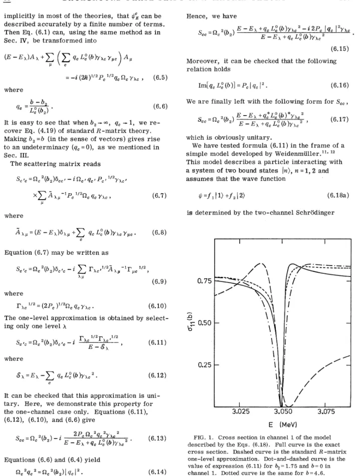
obviously unitary.

We have tested formula

(6.11)

in the frame of a simple model developed by Wej.denmuller.

"'

'

This model describes a particle interacting with asystem of two bound states ln), n =1,2 and assumes that the wave function

"Q&~p 'P.

"'ll.

qcl')„ (6.7)

(6.

18a)

is

determined by the two-channel Schrodinger

&),

„=(&

-&~)~),

_„+Q

q.

L.

'(bb~,

1„,

(6.

8)

Equation (6.7)may be written as S ~

=n

'(b )6 ~ —

iver,

.

"2&,

-'r

(6.

9)

0.

75

r,

.

'"

=

_(2P,

)'"n,

_q,

_~„,.

_(6.10) 1/2_p 1/2

S.

.

.

=n,

'(b, )6.

.

.

—

_(6.11)

where ~x=&~

-Q

_q.

I-.

'(b)rx.

'.

(6.12) It can be checked that this approximation is

uni-tary.

Here, we demonstrate this property for the one-channel case only. Equations

(6.11),

(6.12), (6.10), and

_(6.

6)give

The one-level approximation is obtained by

select-ing only one level ~

0.50

0.

25—

I

3.

025

r ~ r r l l

IiI

! tl

~

3.

050

E {VeV) I

3.

075 2&c

~c'qc'r

_x.

'

Equations (6.6)and (6.4) yield

n,

'q,

'

=n,

'(b,

)lq,

l'.

(6.13)

(6.

14)

FIG.

1.

Cross section in channel 1 of the model

described by the Eqs. (6.18). Full curve is the exact cross section. Dashed curve is the standard R-matrix

one-l.eveI.approximation. Dot-and-dashed curve is the value of expression (6.11) for b&=1.75and b=oin

J.

CUGNON equation

(6.18b)

(6.18c)

Moreover, the functions

_V„(r)

= V

„(r)

have a square well shape

(6.18d) (6.18e) We choose the parameters

r,

=6fm,

e, =0, e,

=6

MeV,

V»=-31

MeV,

V»=-41

MeV,

=

-0.

1MeV. The square well

e,

+_{V» has} abound state at F.

=3.

0512MeV. Because of the coupling

V», this state changes into

a

resonance in channel

1.

The

Eqs. (6.

18b)and

(6.18c}

can be solved using

B-matrix

techniques (for the detail,

see

Ref.

3).

Lejeune and Mahaux,

'

intheir study of this model,

stressed

that the one-level approxi-mation ofthe standard A-matrix theory

is

bound

to fail, whenever the hard sphere phase shift

is

different from the background phase shift. Figure 1 shows the comparison between the exact

cross

section, the result ofthe standard

R-matrix

one-level approximation, and the result of Eq. (6.

11).

The parameters

a,

and b, have been chosen same

as

in Ref. 3, namely,

a,

=_{6fm, b,}

_=S,

_(Ez),

c =_{1, 2.} The parameter b, (c

=1}

has been

deter-mined by fitting the background, and

is

equal to

1.

75.

The remarkable feature ofthe result

is

that formula (6.12)not only reproduces the back-ground, but also the width of the resonance. This is probably due tothe fact that for b,

=

S,

, Ip,I&1

as shown by

Eq. (6.

6). We note that the fitting of the background does not uniquely determine the parameter b,

.

In general, there

are

two possible values ofb,

.

In the numerical

case

above, the two values

are

1.

75and

4.02.

The latter one gives a good value for the background and for the width, but does not correctly reproduce the small asym-metry of the resonance, giving a small peak in

the

cross

section below the dip and not above. Gn

the other hand, when the value of

b, is

chosen to reproduce the background, the results

are

almost independent ofb

as

indicated by the dotted curve of

Fig.

1, which corresponds toh (c

=1)=4.

6. We emphasize that, for the standard

B-matrix

one-level approximation, this value ofb yields a good value of the width, but

a

completely wrong

value ofthe position of the resonance and of the background. It should, homever, be noticed that

the most sophisticated versions of

8-matrix

theory yield more satisfactory one-level approximation generally by including more than the hard sphere in the external region.

In both theories (standard A matrix and present theory), the inner wave function

for

the one-level approximation is practically the same

(i.

e.

,

pro-portional to

X~}.

Hence, it may be surprising that the two theories give quite different results, specially outside the resonance. We show that this difference comes from the prescription used to obtain the scattering matrix from the internal

wave function. The prescription in our theory is different from that used in standard

8

matrix, and it actually generalizes the latter, as we will

see

below. The dynamical

Eqs.

(3.

8)show that the external wave function

is

related to the in-ternal wave function by

@4=4:"'+

~,

& (h.

)PP,

(6»)

or

c Sc' d c

(6.

20b)

This prescription generalizes the one used in standard R-matrix theory. The latter can be

re-covered by dividing Eq.

(6.

20b) by h, and making

6,

tend towards infinity. One finds easily

(6.

21) Sc'

which amounts to equating the external and the internal wave functions on the

surface.

The theory of Lane and Hobson,

'

when applied toB-matrix-type theories,

is

entirely based on

Eqs.

(4.

1)

and (6.

21).

The argument above shows that this

is

equivalent to the Eqs. (4.2)and that the theory of Lane and Hobson is implicitly con-tained in our formalism. We check that

prescrip-tion (6.20) correctly reproduces the collision matrix for the one-level approximation. The in-ternal wave function is given by Isee Eq. (6.

5)]:

(6.22) where the function g',

"'

has a logarithmic deriva-tive equal to

b,

on the

surface.

We multiply Eq.

(6.

19)by g+(b,)on the

left.

We have, with the help

of Eq.

(4.

10) (for b, replacing infinity in the argu-ment of

2),

BACKGROUND

PHASE

SHIFT

IN

R-MATRIX

THEORY

299 and we write Qg as

Qf=

_~

(I,

b„i

—

_S„i

_O,

_i)P,

c Uc' Hence,

(6.

23) b,

—

1

(4.

IPI& 0„..«

b-b,

_'

(0, I»/)

Qc~

a,

.

I«'

E

E„+—

P

_q, Lo(b) y~,

'

~c'

[L,

'

(b,

)*I,

(a,

)6„.

-S„L,

o(b,

)0,

(a,

)].

c~VVc

(6.

25)

S„=Oc

'(bo)

«(2P.

)"'q.

&.

y.

.

(2P.

)"'q.

&.

y~.

E

-Ex+2

q. L:(b)y~.

'

(6.

27)

which is exactly Eq. (6.

11).

This shows, however, that using the continuity condition in the derivation of the collision matrix from the internal wave

function is not a trivial choice

as

it might appear from the standard derivation ofR-matrix theory. We finally make

a

remark on the one-level ap-proximation in the one-channel

case.

It

is

known, in standard

R-matrix

theory, that the one-level approximation yields an exact result at

E =Eq.

This is related to the fact that the inner wave

function is then equal to

Xz.

"

We show that this result remains in our theory. Indeed,

Eqs. (6.11)

gives

S,

.

(E„)=a,

'(b,

)—

i2P,

q, Q,

c

(6.

26)

or,

with the help of

Eqs. (6.

4)and

_(6.

6)

Equations

(6.

24) and

(6.

25) yield

[L:

(b,

)]*I.

(a

),

L,

'.

(b,

)0,

(a,

.

)

«(b

-b,

)

(2h)'"

P,

.

"'n,

y~,

y„,

.

L,

'

(b,)

0,

(a,

.

)

E

E«,

+P

q—

,

I,

'(b)y„,

'

(6.

26) and, with the help of

Eqs.

(6.4)and (4. 18),

VII. CONCLUSIONS

We have formulated the

R-matrix

theory in terms ofprojection operators, and have shown

how to do the same

for

other R-matrix-type

theo-ries.

We find two advantages of such a reformu-lation.

Firstly,

it provides auseful tool to com-pare different theories with each other, since we have a general formalism for all those

theories.

Secondly, we have exhibited the mathematical origin of the arbitrariness in the R-matrix theory

and of the appearance of the hard sphere phase shift in this theory. Particularly, we have shown

that the nonresonant collision matrix is quite arbitrary, and that one can choose any other uni-tary diagonal collision matrix instead of the hard sphere collision matrix. We have constructed a new theory making advantage of this freedom. We have proved on anumerical example, that the one-level approximation in this theory can yield agood description of the background. This is an alternative to the one-level plus constant back-ground approximation in standard

R-matrix

theo-ry or to one-level approximation of sophisticated

R-matrix

theory where the external region con-tains

a

part of the nuclear interaction.

We

are

grateful to

Professor

C. Mahaux for helpful discussions. APPENDIX (

),

[L,

'(b,

)]*L,

'(b) —2«P,(b—b,) cc X c _Lo(b )Lo(b)

„.

L.

'(b,

)[L.

'(b)]*

c _{Lo(b )Lo(b )}

(6.

29)

P=P

+P',

(A1)

Here, we derive the

R-matrix

equations when a few levels

are

treated on a separate footing. Let us divide the

P

space in two subspaces

which is obviously independent of

b,

and

is

equal to the result ofstandard

R-matrix

theory.

where

P'

projects

on the retained levels (X,««) and

300

J.

CUGNON can be written as

[E

—

P'HP'+2

(b)]

P'

rPz——

Z,

(b)Qgs,

[E

—

P'HP'+Z

(b)]

P'gs

=

_g,

_(b)Qg's, (A2) (A3)

Equations (A2) and (A6) yields

[E P-'HP'+Z

(b) S-, (b)O'Z, (

)]P'y',

=Z,

(b)X',&'&

.

_(Alo)

E

—QHQ+&, ( ) 1

*+(

)

_E-PoHPO+Z

(b) +( ) Q~'

=& (")P'O'E _(A5) The solution of this equation

is

Qtjr=

X"

+ O'Z (~

)P'

gs,

(A6) where X,

"

is

the solution of the homogeneous equation obtained from (A5) by setting the right-hand side equal to

zero.

The Green's function

IE —QHQ+&,( )jQPs=& ( )P'4's

+Z

(~)P'qs.

(A4) Let us

first

eliminate

P'.

Equations (A3)and (A4)

yield

Byprojecting on the basis spanned by the Xz, we have

(E —Eg)&), Q-&&g~&,(b)O'2 (

)~&„)A„

=&X,

]Z,

(b)iX',&"& .

(All)

We now need a representation for

8'

and X',

"'.

It is easy to

see

that the operator whose inverse is involved in

Eqs.

(A8)and (AB)is diagonal in the energy indices, when sandwiched between

_g

(E)

and

g~(E').

Using this fact, and the results (4.12) to (4.17), it can be shown that the Green's func-tion

8',

when sandwiched between aZ+ operator on the left and a g operator on the right

[as

in Eq. A(10)] is given by

O' =

_E

—QHQ+2+( ₎—«2

_(~)

1 -1

"E-P~~.

Z (b)

'"'

can be written in the form

g+ 1

E'

—

_QHQ+g,

_{( )} 1

E-P'HP'+Z,

(b) (A7) x

_Q

[1

—

_R'L'(b)]

„

i CII

Similarly the function X'o"'

_is

_{given by} X",

"

=0, P,

"'g

[1

-R'L'(b)]

„i

1 -1

xg,

b

E'-QHQ+ L( ) (A8) Clt —_&/2II yc&+) _(A13)

Similarly, the function Xo'

is

also given by

1 &" ~=&~ ~

'-'-'

)E-WP"~(b)

In the last two equations,

8'

is given by

gO

~

~GC ~GC

CC

0 (A14)

1

+( )_E+

QHQ

g

( ) Using

Eqs.

(A12)and (A13)and the results (4.12) to (4. 17), it is easy to see that Eq. (A12)reduces to

(E —E&)A

_&+P

g

L (b)y& [1 —ROL (b)] ~

y„A&

——

i(25)

~ Pc -Q~

g

(1

-R

L

)«

~

y&,

i,

«

C

(A15)

BACKGROUND

PHASE

SHIFT

IN

8

-MATRIX THEOR

Y 301

*Chercheur Institut Interuniversitaire des Sciences Nucleaires, Belgium.

~_Present address: Division de Physique Theorique, IPN, BPNo. 1, 91-0rsay, France.

~A.M. Lane and R.G.Thomas, Rev. Mod. Phys. 30,

257 (1958).

2C. Mahaux and H.A. Weidenmull, er, Shell-Model

Approach to

¹eleaw

Reactions (North-Hol. l.and,

Am-sterdam, 1969).

3A. Lejeune and C.Mahaux, Nucl. Phys, A145, 613

(1970).

4A.M. Lane and D.Robson, Phys. Rev. 151, 774 (1966). ~H.Feshbach, Ann. Phys. (N.Y.} 19, 287 (1962).

We do not include the point a~=a, . The

P

and Q com-mute with H and

P

+@=1,in the sense that

&PkP+g)lg) =_{&gll[g) for any& and g, except for}

distributions centered at a~. We could include the

point r~=a~. Then,

P

+@=1also holds for

distribu-tions. The projectors P, Q do not commute with H any more, but they do with H+S(b) [see Eq. (3.6)].

We are led, however, tothe same result (4.5). We

choose the first method, excluding

r

= a from the

projectors

P

and Q, because itinvolved the continuity

condition ona more natural. way. 7C._Bloch, Nucl. Phys. 4, 503 (1957).

P. I,.Kapur and R.

E.

Peierl.s, Proc. R. Soc.Lond. A166, 277 (1938).

9L. Garside and W.Tobocman, Phys. Rev. 173, 1047

(1968).

~OR.

J.

_{Philpott and}

J.

_{George, to be published.}

H. A.Weidenmuller, Ann. Phys. (N.Y.)29, 60 (1964). H.A.Weidenmull. er, Ann. Phys. (N.Y.)29, 378(1964).