HAL Id: tel-01821874
https://tel.archives-ouvertes.fr/tel-01821874
Submitted on 23 Jun 2018
HAL is a multi-disciplinary open access
archive for the deposit and dissemination of
sci-entific research documents, whether they are
pub-lished or not. The documents may come from
L’archive ouverte pluridisciplinaire HAL, est
destinée au dépôt et à la diffusion de documents
scientifiques de niveau recherche, publiés ou non,
émanant des établissements d’enseignement et de
quantitative
Guillaume Sall
To cite this version:
Guillaume Sall. Quelques algorithmes rapides pour la finance quantitative. Algorithme et structure de
données [cs.DS]. Université Pierre et Marie Curie - Paris VI, 2017. Français. �NNT : 2017PA066474�.
�tel-01821874�
É
COLED
OCTORALE DES
CIENCESM
ATHÉMATIQUES DEP
ARISC
ENTRET
HÈSE DE
D
OCTORAT
en vue de l’obtention du grade de
Docteur ès Sciences de l’Université Pierre et Marie Curie
Discipline: Mathématiques Appliquées
présentée par
G
uillaume
S
ALL
Quelques Algorithmes Rapides pour la Finance
Quantitative
dirigée par
G
illes
P
AGÈS et
O
livier
P
IRONNEAU
Rapportée par
Mike GILES
Université d’Oxford
Denis TALAY
INRIA
Soutenue le 21 Décembre 2017 devant le jury composé de
Youssef ALLAOUI
Global Market Solutions
Encadrant
Julien BERESTYCKI
Université Pierre et Marie Curie
Examinateur
Gilles PAGÈS
Université Pierre et Marie Curie
Directeur de thèse
Olivier PIRONNEAU
Université Pierre et Marie Curie
Co-Directeur de thèse
Quelques Algorithmes Rapides pour la Finance
...
Quantitative
Contribution au Calcul du Risque de Contrepartie
v Laboratoire de Probabilités et Modèles Aléatoires 4, Place de Jussieu 75005 Paris France Tél. +33 1 44 27 53 19
Global Market Solutions R&D Center
7, Cité de l’Ameublement 75011 Paris
France
vii
Université Pierre et Marie Curie 4, Place de Jussieu
75005 Paris France
Tél. +33 1 44 27 44 27
Laboratoire Jacques Louis-Lions 4, Place de Jussieu
75005 Paris France
. . .À ma mère et mes deux frères.
“La seule chose que je sais, c’est que je ne sais rien.”
“˘εν o˜ιδα ˘oπ o ˙υδ`εν o˜ιδα”
Remerciements
Je tiens particulièrement à exprimer ma gratitude envers mes directeurs de thèse, Gilles Pagès et Olivier Pironneau, pour leur gentillesse et leur disponibilité ainsi que pour les conseils qu’ils m’ont prodigués tout au long de cette thèse. Ce fut un honneur pour moi que Gilles Pagès accepte de diriger cette thèse. Je le remercie pour son temps, le partage de son expérience et son engagement dans ce projet. Je ne remercierai jamais assez Olivier Pironneau pour m’avoir appuyé dans les démarches et sans qui ce projet n’aurait jamais abouti. J’ai énormément appris
sur le plan professionnel et sur le plan humain à leurs côtés. Je les remercie pour m’avoir
rassuré pendant les moments de doutes que j’ai traversé ces dernières années et pour leur grande pédagogie.
L’histoire de cette thèse a commencé chez Global Market Solutions et je tiens beaucoup à remercier Youssef Allaoui et Laurent Marcoux pour leur confiance. Ils ont toujours été présents pour mes questions et m’ont laissé une grande liberté dans ma recherche pour mes travaux. Je tiens à remercier Dominique Vignaux pour avoir accepté ce partenariat entre l’université et Global Market Solutions ainsi que Nathalie Aldini et Tania Corbay pour les démarches administratives. Je remercie également mes anciens collègues de bureau Pierre Weirich, Brahim Ait Haddou, Karim Tamarzist, Brahim Maatalla, Hervé Galicher, Olivier Lamourelle, Aleksey Larchenko et Yassine Sabbahi pour toutes les discussions autour des mathématiques et de la finance, leurs conseils, échanges et collaborations enrichissantes.
Je suis très honoré que Mike Giles et Denis Talay aient accepté de rapporter ma thèse. Je les remercie pour leur lecture attentive de ce manuscrit et l’intérêt porté à mon travail. Je remercie Julien Berestycki pour avoir accepté de présider le jury de ma soutenance de thèse.
Ce projet collaboratif a fait intervenir plusieurs entreprises. Je tiens à remercier les partenaires de chez Intel, Raphaêl Monten qui nous a très gentiment appuyé tout au long de ce projet et nous a mis à disposition le matériel adéquate et les ressources humaines nécessaires. Mais aussi Laurent Duhem, Ayal Zaks, Dahnken Christopher, Hans Pabst et Wolfgang Rosenberg pour leurs aides dans l’implémentation des différentes solutions. La réalisation d’une solution avec 6 cartes Intel Xeon Phi Coprocesseurs a été permise grâce à la collaboration de 2CRSI et de son équipe de développement: Karim Gasmi, Frédéric Mossman, Adrien Badina ainsi que Claire Chupin. Je remercie Massimiliano Fattica de chez Nvidia, pour son aide dans l’implémentation de la solution en CUDA. Je remercie également Arnaud Renard pour nous avoir laisser travailler sur le super calculateur de la région Champagne-Ardenne situé à l’université de Reims. Je souhaite particulièrement remercier Jacques Portès pour toutes les discussions autour de l’architecture des cartes accélératrices et graphiques, ainsi qu’à Alain Dominguez pour ces passionnantes sessions d’implémentation et d’échanges.
La vie au laboratoire est assez particulière et je tiens à remercier tous mes collègues doctorants et notamment ceux de mon bureau à qui j’ai rendu la vie un peu difficile! C’est-à-dire Nicolas Cagniart, Olivier Graf, Antonin Prunet et Guillaume Levy. Mais également ceux qui ont partagés ma vie au laboratoire Anouk Nicolopoulos, Jean François Abadie, Léo Girardin, Cécile Taing, Lilian Gaudin, Lucile Mégret, la liste étant non-exhaustive . . .
Je tiens à remercier tout le personnel des secrétariats des deux laboratoires où j’ai intéragi et notamment Salima Lounici, Malika Larcher et Catherine Drouet au LJLL ainsi que Serena Benassu et Florence Deschamps au LPMA pour leur gentillesse et serviabilité.
Pour finir, une dernière pensée pour mes proches et amis qui ont toujours été présents pour moi. Et particulièrement ma mère Catherine pour sa confiance et son amour, mon petit-frère Thibault pour son soutien indéfectible et qui est aussi un modèle pour moi, mon grand frère Thomas pour avoir toujours cru en mes capacités.
...
Quantitative
Contribution au Calcul du Risque de Contrepartie
Résumé
Dans cette thèse, nous nous intéressons à des noeuds critiques du calcul du risque de contrepartie, la valorisation rapide des produits dérivées et de leurs sensibilités. Nous proposons plusieurs méthodes mathématiques et informatiques pour répondre à cette problématique. Nous contribuons à quatre domaines différents: une extension de la méthode Vibrato et l’application des méthodes multilevel Monte Carlo pour le
calcul des grecques à ordre élevé (n ≥ 1) avec une technique de différentiation
au-tomatique. La troisième contribution concerne l’évaluation des produits Américain, ici nous nous servons d’un schéma pararéel pour l’accélération du processus de val-orisation et nous faisons également une application pour la résolution d’une équation différentielle stochastique rétrograde. La quatrième contribution est la conception d’un moteur de calcul performant à architecture parallèle.
Mots clés : Risque management, Mesures de risques, Sensibilités, Monte Carlo, Monte Carlo multilevel, Monte Carlo multilevel avec poids, Vibrato, Différentiation automatique, Pararéel, In-tégration parallèle en temps, Option Américaine, Option barriére, Option exotique, Valorisation non-linéaire, Monte Carlo avec régression par Moindres carrés, Fonction discontinue, Régulari-sation, ParalléliRégulari-sation, Calcul sur GPU, Grille de noeuds de calcul.
Some Fast Algorithms for Quantitative Finance
Contribution to the Computation of Counterparty Credit Risk
Abstract
In this thesis, we will focus on the critical node of the computation of counterparty credit risk, the fast evaluation of financial derivatives and their sensitivities. We propose several mathematical and computer-based methods to address this issue. We have contributed to four areas: an extension of the Vibrato method and an application of the weighted multilevel Monte Carlo for the computation of the greeks for high
order derivatives (n ≥ 1) with automatic differentiation. The third contribution
concerns the evaluation of American style option, here we use a parareal scheme to speed up the assessing process and we made an application for solving backward stochastic differential equations. The last contribution is the conception of an efficient computation engine for financial derivatives with a parallel architecture.
Keywords : Financial securities, Risk Assessment, Risk Measures, Greeks, Monte Carlo, Multilevel Monte Carlo, Weighted Multilevel Monte Carlo, Vibrato, Automatic Differentiation, Parallel-In-Time Integration, Parareal, American Option, Barrier Option, Exotic Option, Non-linear Pricing, Least Square Monte Carlo, Non-Smooth Function, Regularization, Parallelization, GPU computing, CPUs Cluster.
Nous mentionnons ici les contributions issues de la thèse, qui seront détaillées dans leur intégralité dans les chapitres 1, 2, 3 et 4.
• G. Sall. Approximation of a forward backward stochastic differential equation with a
parareal method. In preparation.
• G. Pagès, G. Sall. Computing sensitivities with weighted multilevel Monte Carlo. In preparation.
• G. Pagès, O. Pironneau, G. Sall. 2017. Vibrato and automatic differentiation for high
order derivative and sensitivities of financial options. Risk Magazine, The Journal of
Com-putational Finance.
• G. Pagès, O. Pironneau, G. Sall. 2016. Second sensitivities in quantitative finance. ESAIM. Proceedings and Surveys. Volume 1, pages 1–10.
• G. Pagès, O. Pironneau, G. Sall. 2016. The parareal method for American options.
Else-vier. Comptes Rendus Mathématiques de l’Académie des Sciences. Volume 354, Issue 11, pages 1132–1138.
Table des Matières
Preface iii
Institutions . . . v
Remerciements . . . xiii
Résumé/Abstract . . . xiv
Contributions Issues de la Thèse . . . xvi
Liste des Figures . . . xxii
Liste des Tables . . . xxiv
Liste des Algorithmes . . . xxv
Liste des Codes . . . xxvi
Liste des Abréviations . . . xxix
Avant-Propos 1 Préambule 3 Introduction 5
Around Computation of Sensitivities
7
1 Vibrato and Automatic Differentiation for High Order Derivatives 9 1.1 Introduction . . . 91.2 Vibrato . . . 12
1.2.1 Vibrato for a European Contract . . . 13
1.2.2 First Order Vibrato . . . 13
1.2.3 Antithetic Vibrato . . . 15
1.2.4 Second Order Derivatives . . . 15
1.2.5 Antithetic Transform, Regularity and Variance . . . 18
1.2.6 Higher Order Vibrato . . . 20
1.3 Second Derivatives by Vibrato plus Automatic Differentiation (VAD) . . . 20
1.3.1 Automatic Differentiation . . . 20
1.3.2 AD in Direct Mode . . . 22
1.3.4 Non-Differentiable Functions . . . 24
1.4 VAD and the Black Scholes Model . . . 25
1.4.1 Conceptual Algorithm for VAD . . . 25
1.4.2 Greeks . . . 25
1.4.3 Numerical Test . . . 25
1.4.4 Basket Call Option . . . 30
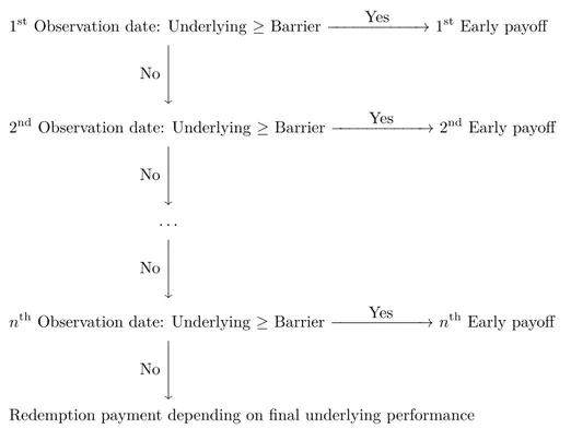
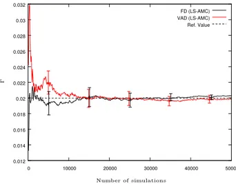
1.4.5 Autocallable . . . 33
1.5 Computation with Vibrato plus Reverse AD (VRAD) . . . 37
1.6 American Option . . . 38
1.6.1 Longstaff Schwartz Algorithm . . . 38
1.6.2 Procedure to Compute the Gamma of an American option . . . 39
1.6.3 Numerical Test . . . 40
1.7 Second Derivatives in a Stochastic Volatility Model . . . 41
1.7.1 Procedure to Compute Second Derivatives in the Heston Model . . . 41
1.8 Malliavin Calculus and Likelihood Ratio Method . . . 44
1.8.1 Numerical Tests . . . 45
1.9 Conclusion . . . 46
2 Computing Sensitivities with Weighted Multilevel Monte Carlo 55 2.1 Introduction . . . 55
2.2 Preliminaries . . . 57
2.3 Multilevel Monte Carlo with Optimal Parameters . . . 59
2.3.1 Multilevel Setting . . . 59
2.4 Weighted Multilevel Monte Carlo Method with Optimal Parameters . . . 62
2.4.1 Richardson-Romberg Extrapolation . . . 62
2.4.2 The Multistep Approach . . . 64
2.4.3 Weighted Multilevel Setting . . . 65
2.5 Antithetic Schemes . . . 71
2.5.1 Truncated Milstein Scheme . . . 71
2.5.2 Optimal Settings . . . 74
2.6 Generic Procedure for Option Pricing and Sensitivities . . . 75
2.7 Numerical Results . . . 79
2.7.1 Computation of Sensitivities of Up and Out Call Option in the Heston model 80 2.7.2 Using the Framework 2.6 for the Value, the Delta and the Gamma . . . . 81
2.7.3 Antithetic Scheme . . . 82
2.8 Conclusion . . . 83
Around Pricing Method
93
3 The Parareal Algorithm for American Options 95 3.1 Introduction . . . 953.2 The Problem . . . 96
3.3 A Two Level Parareal Algorithm . . . 99
3.3.1 The Parareal Method for ODE . . . 99
3.3.2 The Parareal Method for SDE . . . 100
3.4 Multi-level Parareal for SDE . . . 108
Table des Matières
3.5.1 Correcting Markovian deficiency . . . 111
3.5.2 Some Considerations on TLPRAO . . . 113
3.6 Numerical Tests . . . 116
3.6.1 Convergence of the Parareal Algorithm for a SDE . . . 116
3.6.2 Convergence of the Parareal Algorithm For an American Contract . . . . 117
3.6.3 Multilevel Parareal Algorithm . . . 118
3.7 The Iterative Parareal Method and Sensitivities . . . 119
3.7.1 Procedure . . . 120
3.7.2 The Delta in the Black Scholes Model . . . 121
3.7.3 The Delta in the Constant Elasticity of Variance Model . . . 122
3.8 Conclusion . . . 122
4 Approximation of a (F)BSDE with a Parareal Method 129 4.1 Introduction . . . 129
4.2 Nonlinear Option Pricing . . . 130
4.2.1 Decoupled Forward Backward Stochastic Differential Equation . . . 130
4.2.2 The Two Level Parareal Procedure for a Decoupled FBSDE . . . 132
4.3 Numerical Experiments . . . 134
4.3.1 Bid-Ask Spread Option for Interest Rate . . . 134
4.3.2 Numerical Results . . . 134
4.4 Conclusion . . . 135
Travaux Effectués en Entreprise
137
5 Moteur de Calcul Optimisé à Architecture Hybride et Diverse 139 5.1 Introduction . . . 1395.2 Produits Dérivés de Taux d’Intérêt . . . 140
5.2.1 Échange de Taux d’Intérêt (SWAP, IRD) . . . 140
5.3 Intel Xeon-Phi Coprocessor . . . 142
5.4 Optimisation . . . 145
5.4.1 Système d’Exploitation . . . 146
5.4.2 Parallélisme et AoS to SoA . . . 147
5.4.3 Fonctions Mathématiques Spécifiques . . . 149
5.4.4 Vectorisation . . . 150
5.4.5 Affinité des Processus Logiques . . . 151
5.4.6 Architecture Hybride . . . 152
5.4.7 Option de Compilation . . . 154
5.4.8 OpenMP . . . 154
5.4.9 Algorithme du Moteur de Calcul à Architecture Hybride . . . 155
5.5 Tests et Mesures . . . 156
5.5.1 Un Serveur avec Une Carte Accélératrice . . . 156
5.5.2 Un Serveur avec Six Cartes Accélératrices . . . 157
5.6 Un Code, Plusieurs Architectures . . . 160
5.6.1 Carte Graphique . . . 160
5.6.2 Architecture Nvidia et CUDA . . . 161
5.6.3 OpenCL . . . 165
5.7 Expérimentation et Résultat Numérique . . . 169
5.7.1 Architecture Homogène . . . 169
5.8 Conclusion . . . 171
6 Régularisation, Fonction Discontinue et Différentiation Automatique 173 6.1 Introduction . . . 173
6.2 Différentiation Automatique du Premier Ordre sur GPU . . . 174
6.2.1 Structure CUDA Différentiation par Induction . . . 174
6.3 Applications à un Produit Dérivé Européen . . . 175
6.3.1 Call Européen . . . 175
6.4 Différentiation Automatique du Second Ordre sur CPU . . . 176
6.4.1 Structure C++ de Différentiation par Induction . . . 176
6.5 Applications aux Produits Exotiques . . . 178
6.5.1 Power Call (modèle Black Scholes) . . . 178
6.5.2 Option Chooser (modèle Black Scholes) . . . 179
6.5.3 Digital Call Asiatique (modèle Constant Elasticity of Variance) . . . 180
6.5.4 Up & Out Call (modèle Heston) . . . 181
6.5.5 American Put (modèle Black Scholes) . . . 182
6.6 Conclusion . . . 183
A Some Definitions 185
B Semi-Smooth Newton Method 193
C Asynchronous Parallelism 195
D Libor Market Model (LMM) 197
E Résultat de L’Implémentation Visant un Serveur et Six Phi 201
Bibliographie 203
Liste des Figures
1.1 Representation of Vibrato decomposition on a Monte Carlo path . . . 12
1.2 Precision (log-log plot of|dzdu − cos(1.)|) . . . . 21
1.3 Precision (log-log plot of|dzdu − cos(1.)|) complex increments . . . . 22
1.4 Computation of Gamma of an European Call option via VAD . . . 27
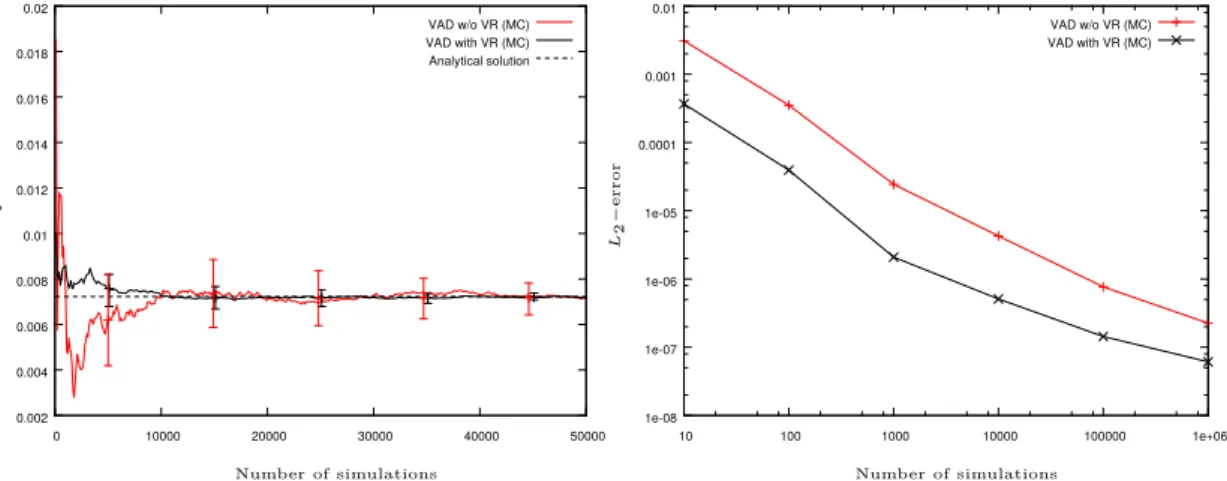
1.5 Variance and L2−error of Gamma computation via VAD . . . . 27
1.6 Computation of Vanna of an European Call option via VAD . . . 28
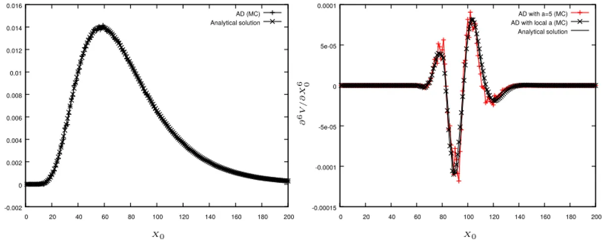
1.7 Computation of third derivatives of an European Call option via VVAD . . . 29
1.8 Approximation of Gamma via AD with a smoothing technique . . . 29
1.9 Computation of Gamma of a Basket Call option (4d and 7d) . . . 33
1.10 Schematic representation of the payoff of an Autocallable . . . 34
1.11 Convergence of Gamma of an American Put option . . . 41
1.12 The Gamma versus price in the Heston model . . . 43
1.13 The Vanna versus price in the Heston model . . . 43
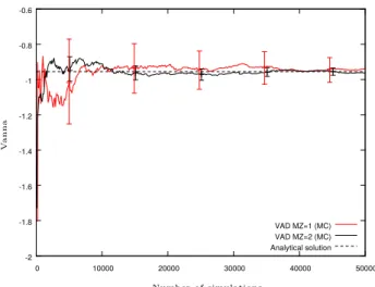
1.14 The Vomma versus price in the Heston model . . . 44
2.1 Representation of the multilevel simulation path . . . 58
2.2 Parameters of the MLMC estimator (standard framework) . . . 63
2.3 Parameters of the ML2R estimator (standard framework) . . . 70
2.4 Parameters of the MLMC estimator (antithetic scheme) . . . 74
2.5 Parameters of the ML2R estimator (antithetic scheme) . . . 75
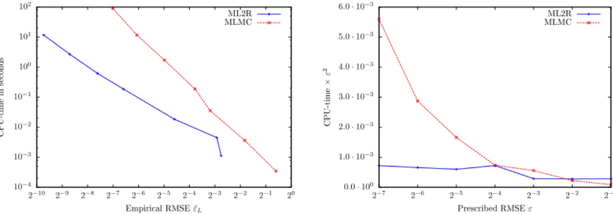
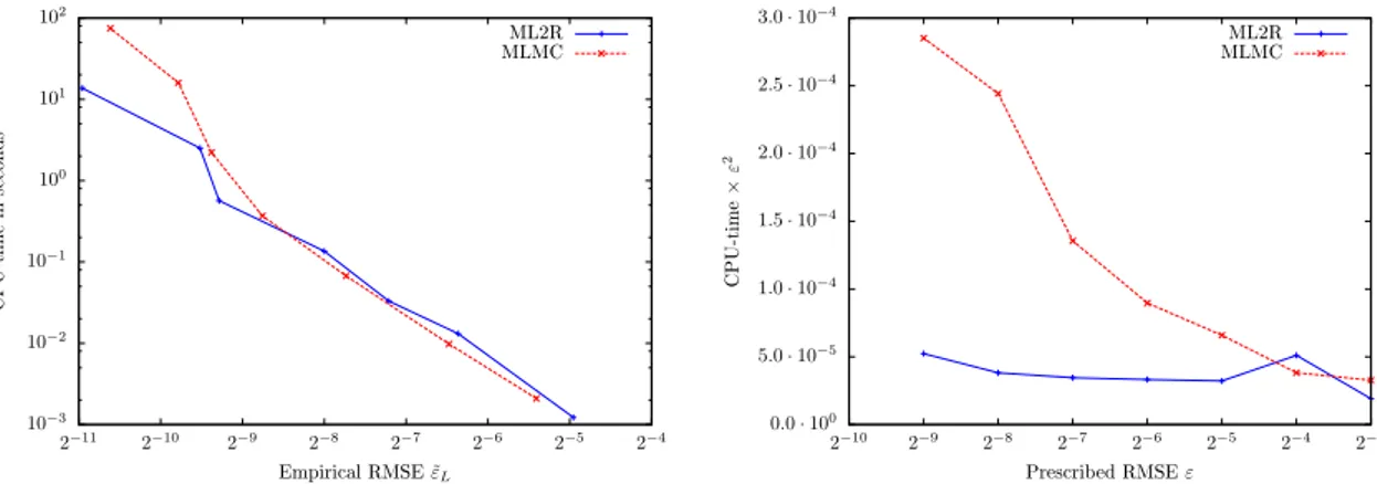
2.6 MLMC/ML2R, (CPU-time vs εL for the Price of UOC) . . . 84
2.7 MLMC/ML2R, (CPU-time vs εL for the Delta of UOC) . . . 85
2.8 MLMC/ML2R, (CPU-time vs εL for the Gamma of UOC) . . . 86
2.9 MLMC/ML2R, (CPU-time vs εL for the Vega of a smooth function) . . . 88
2.10 MLMC/ML2R, (CPU-time vs εL for the Vomma of a smooth function) . . . 89
3.1 Schematic representation of the two level parareal algorithm . . . 123
3.2 Simulation paths of an SDE at different parareal iterations . . . 124
3.3 BS model: absolute error of an American Put option . . . 124
3.4 CEV model: absolute error of an American Put option . . . 125
3.5 Comparison between a standard and the parareal LSMC (American option) . . . 125
3.7 BS model: absolute error of the Delta of an American Put option . . . 126
3.8 CEV model: absolute error of the Delta of an American Put option . . . 127
4.1 FBSDE: absolute error of a Bid-Ask Spread Call option . . . 135
4.2 Comparison between a standard and parareal LSMC (Call Spread option) . . . . 136
5.1 La carte Intel Xeon Phi Coprocessor . . . 142
5.2 L’architecture de l’Intel Xeon Phi Coprocessor . . . 144
5.3 Processus d’optimisation . . . 147
5.4 Représentation du parallélisme . . . 148
5.5 Restructuration des données . . . 148
5.6 Schéma des accès en mémoire . . . 149
5.7 Taille des unités vectorielles . . . 150
5.8 Performance en GFLOPs sur du calcul matriciel . . . 152
5.9 Architecture hexaPhi . . . 153
5.10 Facteur d’accélération . . . 160
5.11 Architecture CPU vs GPU . . . 161
5.12 Représentation d’une grille d’un GPU . . . 162
5.13 Architecture mémorielle d’un GPU . . . 163
5.14 Temps de calculs et facteur d’accélération pour un code OpenCL . . . 170
Liste des Tableaux
1.1 Time computing of the Hessian matrix of an European Call option . . . 38
1.2 Variance of Gamma of an European Call option on different methods . . . 45
1.3 Second derivatives of an European Call option (VRAD vs FD) . . . 47
1.4 Error values for second derivatives (VRAD vs FD) . . . 48
1.5 Second derivatives of an European Call option (VAD vs FD) . . . 49
1.6 Error values for second derivatives (VAD vs FD) . . . 50
1.7 Gamma approximation of a Basket Call option . . . 51
1.8 Time computing of Gamma for a Basket Call option . . . 51
1.9 Results for the price, the Delta and the Gamma of an Autocallable . . . 52
1.10 Delta, Gamma of an American Put option . . . 53
2.1 Price of UOC (ML2R) in the Heston model (α = 0.5, β = 0.5) . . . . 84
2.2 Price of UOC (MLMC) in the Heston model (α = 0.5, β = 0.5) . . . . 84
2.3 Delta of UOC (ML2R) in the Heston model (α = 0.5, β = 0.5) . . . 85
2.4 Delta of UOC (MLMC) in the Heston model (α = 0.5, β = 0.5) . . . . 85
2.5 Gamma of UOC (ML2R) in the Heston model (α = 0.5, β = 0.75) . . . 86
2.6 Gamma of UOC (MLMC) in the Heston model (α = 0.5, β = 0.75) . . . . 86
2.7 Results for framework in the Black Scholes model (ML2R) . . . 87
2.8 Results for framework in the Black Scholes model (MLMC) . . . 87
2.9 Vega (ML2R) in the Clark Cameron model (α = 1, β = 2) . . . . 88
2.10 Vega (MLMC) in the Clark Cameron model (α = 1, β = 2) . . . . 88
2.11 Vomma (ML2R) in the Clark Cameron model (α = 1, β = 2) . . . . 89
2.12 Vomma (MLMC) in the Clark Cameron model (α = 1, β = 2) . . . . 89
3.1 Absolute error with the iterative parareal method (SDE) . . . 117
3.2 Absolute error with the iterative parareal method (American Put) . . . 117
3.3 Absolute error for the price (CEV) with the iterative parareal method . . . 118
3.4 Absolute error with the multilevel parareal method, table 1 . . . 120
3.5 Absolute error with the multilevel parareal method, table 2 . . . 120
3.6 Absolute error for the Delta (BS) with the iterative parareal method . . . 121
4.1 FBSDEl: absolute error of a Bid-Ask Spread Call option . . . 135
5.1 Niveau et correspondance des différents protocols de parallélisation . . . 147
5.2 Puissance théorique en GFLOPs . . . 157
5.3 Temps de calculs pour un portfeuille de SWAPs (SP) . . . 158
5.4 Temps de calculs pour un portfeuille de CAPs/FLOORs (SP) . . . 158
5.5 Temps de calculs pour un portfeuille de SWAPs (DP) . . . 158
5.6 Temps de calculs pour un portfeuille de CAPs/FLOORs (DP) . . . 158
5.7 Temps de calculs sur l’architecture hexaPhi . . . 159
5.8 Energie consommée, prix et empreinte carbone . . . 160
5.9 Temps de calculs avec un code OpenCL et C++ . . . 169
5.10 Performances réalisées sur les architectures . . . 170
6.1 Erreur L2 pour l’approximation du Delta d’un Call Européen . . . 176
6.2 Erreur L2 pour l’approximation du Vega d’un Call Européen . . . 176
6.3 Erreur L2 pour l’approximation du Gamma d’un Power Call . . . 179
6.4 Erreur L2 pour l’approximation du Gamma d’une option Chooser . . . 180
6.5 Erreur L2 pour l’approximation du Gamma d’une Digital sur Call Asiatique . . . 181
6.6 Erreur L2 pour l’approximation du Gamma d’une option Up & Out Call . . . 182
Liste des Algorithmes
1 VAD for second derivatives using antithetic variance reduction . . . 26
2 Framework for the evaluation of sensitivities and price . . . 90
3 Detailed part of steps 16:20 of Algorithm 2 (Heston model, Call option). . . 91
4 BDP-Algorithm . . . 98
5 LSMC-algorithm . . . 99
6 TLPR: Two levels Parareal for SDE . . . 101
7 TLPRAO(A): Two levels Parareal for American Options . . . 109
8 Moteur de calcul pour machine hybride . . . 156
9 Semi-Smooth Newton algorithm . . . 194
Liste des Codes
1.1 Function implemented in C++ . . . 20
1.2 Approximation of the derivative of a function implemented in C++ . . . 21
1.3 Example of forward class implementation in C++ . . . 23
1.4 Example of forward function implementation in C++ . . . 23
5.1 Exemple d’une section offload programmée en C++ . . . 145
5.2 Exemple de boucle de code à vectoriser en C++ . . . 150
5.3 Code 5.2 vectorisé à l’aide de fonctions intrinsèques en C++ . . . 151
5.4 Création des processus logiques avec Posix Threads . . . 153
5.5 Exécution des processus logiques avec Posix Threads . . . 153
5.7 Code CUDA permettant la multiplication d’un vecteur par un scalaire . . . 165
5.8 Code OpenCL permettant l’addition de deux vecteurs . . . 168
6.1 Partie de l’implémentation de la class CudaD . . . 175
6.2 Exemple de surcharge d’opérateur pour la class CudaD . . . 175
6.3 Partie de l’implémentation de la class ddouble (2ème ordre) . . . 177
Liste des Abréviations
AD Automatic Differentiation.
API Application Programming Interface.
ASIC Application Specific Integrated Circuit.
AVX Advanced Vector eXtension.
.
BDP Backward Dynamic Programming.
BLAS Basic Linear Algebra Subprograms.
BSDE Backward Stochastic Differential Equation.
.
BS Black Scholes model.
CDS Credit Default SWAP.
CEV Constant Elasticity of Variance model.
CPU Central Processing Unit.
CSA Credit Support Annex.
CSV Comma Separated Values.
CVA Credit Valuation Adjustment.
CollBA Collateral Venefit Adjustment.
CollCA Collateral Cost Adjustment.
CollVA Collateral Value Adjustment.
.
DF Discount Factor.
DP Double Precision.
DVA Debt Value Adjustment.
.
EEPE Effective Expected Positive Exposure.
EE Expected Exposure.
EPE Eexpected Positive Exposure.
.
FBSDE Forward Backward Stochastic Differential Equation.
FD Finite Difference method.
FLOP FLoating OPeration per seconde.
FRTB Fundamental Review of the Trading Book.
FVA Funding Value Adjustment.
.
GDDR5 Graphics Double Dada Rate type 5.
GPU Gprahic Processing Unit.
.
HBA Hedging Benefit Adjustment.
HCA Hedging Cost Adjustment.
HVA Hedging Value Adjustment.
.
IM Initial Margin.
IRD Interest Rate Derivative.
IRIS Innovative Risk Integration System.
IT Information Technologie.
.
KVA Capital Value Adjustment.
.
LMM Libor Market Model.
LRM Likelihood Ratio Method.
LRPW Likelihood Ratio coupled to Path-Wise method.
LSMC Least Square Monte Carlo.
LVA Liquidity Value Adjustment.
.
MC Monte Carlo method.
ML2R MultiLevel Rrichardson-Romberg extrapolation.
MLMC MultiLevel Monte Carlo.
MMX Multiple Math eXtension.
MPI Message Passing Interface.
MVA Margin Value Adjustment.
MtM Mark-to-Market.
.
ODE Ordinary Differential Equation.
OIS Overnight Index SWAP.
OSS One-Step Survival estimator.
OTC Over-The-Counter.
.
PCA Principal Component Aanlysis.
PCI Peripheral Component Interconnect.
PDE Partial Differential Equation.
PFE Potential Future Exposure.
PW Path-Wise method.
P&L Profit and Loss profil.
.
RIX Risk Intelligence Expression.
RMSE Root Mean Square Error.
.
SA-CCR Standardized Approach for Counterparty Credit Risk.
Liste des Abréviations
SIMD Single Instruction Multiple Data.
SIMM Standard Initial Margin Model.
SIMT Single Instruction Multiple Threads.
SISD Single Instruction Single Data.
SP Simple Precision.
SSE Streaming SIMD eXtension.
.
TLPRAO Two Levels ParaReal for American Options.
.
TLPR Two Levels ParaReal.
UOC Up–Out Call barrier option.
.
VAD Vibrato and Automatic Differentiation (forward mode).
VM Variation Margin.
VRAD Vibrato and Reverse Automatic Differentiation.
VaR Value-at-Risk.
.
Avant-Propos
Avant-Propos
Cette thèse s’effectue dans le cadre d’une collaboration entre l’Université Pierre et
Marie Curie1 (UPMC) et Global Market Solutions (GMS) sous un contrat CIFRE
géré par l’Association Nationale de la Recherche et de la Technologie (ANRT). La thèse s’est effectuée au sein du Laboratoire de Probabilités de Modèles Aléatoires (LPMA) sous la direction de Gilles Pagès et d’Olivier Pironneau, tous deux Pro-fesseurs d’université, et au sein du pôle Recherche et Développement de Global Market Solutions avec l’encadrement de Youssef Allaoui et Laurent Marcoux respectivement directeur technique et manager du pôle front office.
Préambule
“Le marché, à son insu, obéit à une loi qui le domine: la loi de la probabilité”
extract from Théorie de la Spéculation, [9].
− L. Bachelier, Mathématicien, (1870, 1946).
Global Market Solutions est une entreprise de consulting qui propose des implémentations et des solutions d’intégrations de progiciel financier en Europe, Asie et Amérique. L’entreprise s’intéresse particulièrement aux problématiques de front office et à l’intégration de modèle de valorisation d’actifs financiers; du management de risque qui inclus les risques de marché, les risque de crédit, et d’analyse de liquidité en temps réel; aux problématiques de back office.
En 2013, Global Market Solutions a été confronté au problème de valorisation de plusieurs dizaines de milliers de produits dérivés pendant les sessions de calculs de nuit (noeud de calcul pour le risque de contrepartie). Ils se sont tournés vers la parallélisation en réponse à ce problème, ce qui inclus des solutions et l’étude de carte graphique et de nouvelle architecture telle que le Xeon Phi Coprocessor. Dans cette thèse, nous étudions de nouveaux algorithmes rapides et performants pour la valorisation d’actifs financiers, produits dérivés et de leurs sensibilités en utilisant des machines parallèles.
Les méthodes de Monte Carlo sont naturellement parallèles à l’exception de leurs usages dans la programmation dynamique pour la valorisation des produits Américains dans l’algorithme de
Longstaff Schwartz [124]. Des algorithmes de Monte Carlo rapides et efficaces ont déjà été
proposé, indépendamment du parallélisme, comme les méthodes de Monte Carlo multilevel par Giles [61], la méthode de quantification optimale par Pagès et Printems [144], les méthodes de quasi Monte Carlo par Boyle et al. [105] et beaucoup d’autres. . . Pour l’évaluation des sensibilités ou des grecques, dans [60], Giles propose une méthode efficace et performante appelée Vibrato.
Dans cette thèse, nous contribuons dans trois domaines différents: 1/ Vibrato, 2/ Monte Carlo multilevel avec poids, 3/ Accélération pararéelle. Pour répondre à la problématique posée par Global Market Solutions, nous avons étudié les nouvelles architectures qui sont une extension ou vise à remplacer les architectures usuelles i.e. un PC ou une grille standard de CPUs.
Le chapitre 1 est consacré au calcul du second et des ordre supérieurs de dérivation des pro-duits financiers. Nous avons combinés deux méthodes, Vibrato et la différentiation automatique et nous les comparons avec d’autres méthodes de calcul des sensibilités. Nous montrons que cette combinaison de technique est plus rapide et plus stable que la différentiation automatique pour la dérivée seconde ou l’approche par différences finies. Nous proposons un framework générique de calcul de grecques et présentons plusieurs applications à des produits financiers vanilles et
exotiques. Nous étendons également la différentiation automatique pour le calcul de la dérivée second pour la fonctions de payoffs qui ne sont pas dérivable deux fois.
Dans le chapitre 2, nous étudions l’approximation des sensibilités des produits dérivés fi-nanciers avec une méthode multilevel Monte Carlo avec poids. Le calcul des sensibilités utilise une régularisation de la fonction Heaviside pour les payoff financiers. Nous montrons comment calibrer la méthode multilevel pour les grecques en utilisant les paramètres optimaux proposés par Lemaire et Pagès [119] pour des schémas standards et antithétiques. Nous donnons égale-ment un framework qui calcule simultanéégale-ment la valeur de produits financiers et de ses grecques sur une même grille en utilisant les paramètres optimaux. Nous proposons quelques applications sur des produits vanilles et exotiques.
Le chapitre 3 propose une description de la méthode pararéelle pour la valorisation des pro-duits Américains et une section numérique pour évaluer ses performances. Nous étudions unique-ment le cas scalaire. La méthode Monte Carlo avec régression par moindres carrés et la décom-position pararéelle en temps avec deux et plusieurs niveaux sont utilisées pour le développement d’une implémentation parallèle efficiente. Nous proposons également un argument de conver-gence pour l’algorithme à deux niveaux lorsque le pas de temps pour le schéma d’Euler à chaque niveau est approprié. Cet argument de convergence nous servira pour l’analyse du cas à plusieurs niveaux.
Le chapitre 4 est une extension du chapitre précédent. Nous faisons une application de la méthode pararéelle pour l’approximation de la solution d’une équation différentielle stochastique rétrograde (BSDE) pour la valorisation d’un produit financier i.e. Bid-Ask Spread Call option pour les taux d’intérêt. La méthode de Monte Carlo avec régression par moindres carrés est un choix populaire pour l’approximation ce type d’équation. Le schéma de discrétisation a une complexité assez élevée puisqu’il nécessite l’approximation d’au moins deux espérances condi-tionnelles. L’utilisation des schémas pararéels est donc une bonne méthode pour la résolution des équations différentielles stochastiques rétrogrades.
Le chapitre 5 est dédié au travail réalisé au sein de Global Market Solutions pour la conception d’un moteur de calcul efficient et rapide pour le calcul massif de produits dérivés de taux. Ce travail s’inscrit en réponse aux demandes croissantes d’indicateurs de risques, la valorisation rapide des portefeuilles de produits financiers est devenu un enjeu majeur pour les banques. Le moteur de calcul repose sur une architecture parallèle à mémoire partagée et distribuée. Nous verrons comment profiter de tous les types de granularité de parallélisation en vue de bénéficier de toutes les capacités des différentes architectures. Nous procédons à plusieurs tests numériques pour prouver l’efficacité de l’implémentation.
Dans l’annexe 6, nous présentons les librairies de différentiation automatique qui ont été implémentées dans le cadre de la collaboration avec Global Market Solutions et qui ont servies aux expérimentations faîtes dans les chapitres 1, 2 et 3. Ces librairies ont également été utilisées dans le cadre de test numérique interne et de la faisabilité de l’intégration de telles libraires dans IRIS (progiciel de calcul de risque développé par Global Market Solutions) au sein du département de recherche & développement de l’entreprise partenaire. Nous présentons succinctement les
deux librairies implémentées i.e. une version C++ pour le calcul du premier et du second
ordre de dérivation ainsi qu’une version CUDA destinée aux cartes graphiques pour le calcul du premier de dérivation. Nous faisons une rapide description de la régularisation utilisée. Quelques applications en finance sont présentées à titre illustratif sur des produits vanilles et exotiques dans plusieurs modèles stochastiques.
Introduction
2
Global Market Solutions operates as a consulting company that engages implementation and integrates financial software projects in Europe, Asia, and the Americas. The company primarily focuses on front office and pricing model integrations; risk management that includes market risk, credit risk, and liquidity risk analysis, as well as real-time monitoring; back office and straight through processing; and accounting and regulatory monitoring.
In 2013, Global Market Solutions was confronted with the problem of evaluating several thousands of derivatives overnight. They turned to parallel computing for an answer, this includes GPU cards in a PC and new chips like the Xeon Phi Coprocessor. In this thesis, we investigate faster algorithms for pricing assets, derivatives and their sensitivities the so-called greeks, using parallel machines.
The Monte Carlo method is naturally parallel except when dynamic programming is used as in the Longstaff Schwartz [124] for American options. Fast Monte Carlo algorithms have been proposed independently of parallelism such as multilevel Monte Carlo Giles [61], optimal quantization Pagès et Printems [144], quasi Monte Carlo methods by Boyle et al. [105] and many more. . . For the computation of greeks, in [60], Giles proposed an acceleration which is called Vibrato.
In this thesis, we have contributed to four areas: 1/ Vibrato, 2/ Weighted multilevel, 3/ Parareal acceleration. To answer the challenge of global Market Solutions, we have investigated the new architectures to extend or replace single PC and PC clusters, this is our fourth contri-bution.
The chapter 1 deals with the computation of second or higher order Greeks of financial securities. It combines two methods, Vibrato and automatic differentiation and compares with other methods. We show that this combined technique is faster and more stable than automatic
differentiation of second order derivatives or finite difference approximations. We present a
generic framework to compute any Greeks and present several applications on different types of derivatives. We also extend automatic differentiation for second order derivatives of non-twice differentiable payoff.
In chapter 2, we study the approximation of the sensitivities of financial derivatives with a weighted multilevel Monte Carlo. The computation of sensitivities are made with an extended version of automatic differentiation for non-twice differentiable payoff using a regularization of the Heaviside function. We show how to calibrate the method for sensitivities using the optimal framework designed by Lemaire and Pagès in [119] for standard and antithetic discretization scheme. Also, we give a description of a framework which compute the value, Delta and Gamma
of a security using the optimal parameters for each function on the same grid. We give some numerical results on vanilla and exotic derivatives.
The chapter 3 gives a description of the parareal method for American contracts, a numerical section to assess its performance. The scalar case is investigated. Least Squares Monte Carlo (LSMC) and parareal time decomposition with two or more levels are used, leading to an efficient parallel implementation. It contains also a convergence argument for the two levels parareal Monte Carlo method when the time step used for the Euler scheme at each level is appropriate. This argument provides also a tool to analyze the multilevel case.
Chapter 4 is an extension of the previous chapter. We apply the parareal method to the approximation of a backward stochastic differential equation with an application to the pricing of a Bid-Ask Spread option for interest rates. The Least squares Monte Carlo method is a popular choice to approximate the solution for these equations. The discretization scheme is quite complex because there are at least two conditional expectations to evaluate. Hence, the parareal algorithm is a good method for solving backward stochastic differential equations.
The chapter 5 is dedicated to the work accomplished at Global Market Solutions for the design of an efficient calculation engine of rate derivatives. Fast portfolio assessing has become a major issue for financial institutions and banks, this work propose an answer to the growing demands in the number of risk measures. This engine calculation was written on a parallel architecture with distributed and shared memory. We will see how to use different type of parallelism granularity to benefit from every architectures have shown. We made several experiments to analyze and assess the performance.
In appendices 6, we present the different automatic differentiation libraries made during the collaboration with Global Market Solutions and which have been used in the chapters 1, 3 et 2. These libraries have been used for testing the possibility to integrate them inside IRIS (professional software to compute risk measures developed by Global Market Solutions). We briefly introduce the two libraries in C++ (up to 2nd order of derivation) and CUDA (1st order of derivation) on CPU and GPU. We make a short description of the implementation of the regularization for non smooth payoff. We make several applications to vanilla and exotic financial products in several simulation stochastic models.
.
Around Computation of
Sensitivities
Chapitre 1
Vibrato and Automatic
Differenti-ation for High Order Derivatives
and Sensitivities of Financial
Op-tions
“La puissance de l’automatisation est telle que ses progrès mécaniques s’étendent aussi bien dans les contrées où la main d’œuvre est encore à vil prix, que dans les pays où le prix du
travail manuel s’élève constamment”
− M. Alcan, Politician, (1810, 1877).
This chapter deals with the computation of second or higher order Greeks of financial secu-rities. It combines two methods, Vibrato and automatic differentiation and compares with other methods. We show that this combined technique is faster and more stable than au-tomatic differentiation of second order derivatives or finite difference approximations. We present a generic framework to compute any Greeks and present several applications on different types of derivatives. We also extend automatic differentiation for second order derivatives of non-twice differentiable payoff.
.
This chapter is an extended version of the article Pagès et al. [143] published in Risk Journal,
The Journal of Computational Finance.
1.1
Introduction
Due to BASEL III regulations, banks are requested to evaluate the sensitivities of their port-folios every day (risk assessment). Some of these portport-folios are huge and sensitivities are time consuming to compute accurately. Faced with the problem of building a software for this task and distrusting automatic differentiation for non-differentiable functions, we turned to an idea developed by Mike Giles called Vibrato.
Vibrato at core is a differentiation of a combination of likelihood ratio and pathwise evalu-ation. In Giles [60] and [62], it is shown that the computing time, stability and precision are enhanced compared with numerical differentiation of the full Monte Carlo path.
In many cases, gamma hedging being one, double sensitivities, i.e. second derivatives with respect to parameters, are needed. The purpose of this chapter is to investigate the feasibility of Vibrato for second and higher derivatives. We will first compare Vibrato applied twice with the analytic differentiation of Vibrato and show that it is equivalent; since the second is easier, we propose the best compromise for second derivatives: Automatic Differentiation of Vibrato.
In [40], Capriotti investigated the coupling of different mathematical methods – namely path-wise and likelihood ratio methods – with an Automatic differentiation technique for the compu-tation of second order Greeks; here we follow the same idea but with Vibrato and also for the computation of higher order derivatives.
Automatic Differentiation (AD) of computer program as described by Griewank [81], Griewank and Walther [82], Naumann [137] and Hascœt [87] can be used in direct or reverse mode. In direct mode the computing cost is similar to finite difference approximation but with no roundoff errors: the method is exact because every line of the computer program which implements the financial option is differentiated exactly. The computing cost of a derivative of order n with respect to a single parameter is similar to running the program n times. Evaluation of all partial derivatives with respect of a vector valued parameter is substantially more expensive and requires the so-called reverse mode of AD.
For many financial products the first or the second sensitivities do not exist at some point, such is the case for the standard Digital option at x = K; even the payoff of a plain vanilla European option is not twice differentiable at x = K, yet the Gamma is well defined; in short, the end result is well defined but the intermediate steps of AD are not.
We tested ADOL-C of Griewank and Walther [83] and tried to compute the Hessian matrix for a standard European Call option in the Black Scholes model but the results were wrong. So we adapted our AD library based on operator overloading by including approximations of Dirac functions and obtained decent results; this is the second conclusion of the chapter: AD for second sensitivities can be made to work; it is simpler than Vibrato+AD (VAD) but it is slightly more computer intensive and risky because the precision depends on the right choice of the parameter which appears in the approximation of a Dirac function by an exponential.
More details on AD applied to quantitative finance can be found in Giles and Glasserman [58], Pironneau [154], Capriotti [39], Homescu [96] and the references therein.
An important constraint when designing professional software for risk assessment is to be compatible with the history of the company which contracts the software; most of the time, this rules out the use of partial differential equations to compute sensitivities (see Achdou and Pironneau [2]) as most quant companies use Monte Carlo algorithms for pricing their portfolios. For security derivatives computed by a Monte Carlo method, the computation of their sensi-tivities with respect to a parameter is most easily approximated by finite difference (also known as the shock method) thus requiring the reevaluation of the security with an incremented pa-rameter. There are two problems with this method: it is imprecise when generalized to higher order derivatives and expensive for multidimensional problems with multiple parameters. The
nthderivative of a security with p parameters requires (n + 1)p evaluations (and more if
cross-derivatives are required); furthermore the choice of the perturbation parameter is delicate as it should be neither too large nor too small, as explained in section 1.3.1.
From a semi-analytical standpoint the most natural way to compute a sensitivity is the pathwise method described in Glasserman [71] which amounts to compute the derivative of the payoff for each simulation path. Unfortunately, this technique happens to be inefficient for certain
1.1. Introduction
types of payoffs including some often used in quantitative finance like Digitals or Barrier options. For instance it is not possible to obtain the Delta of a Digital Call that way because the derivative of the expectation of a Digital is not equal to the expectation of the derivative. The pathwise derivative estimation is also called infinitesimal perturbation and there is a extensive literature on this subject; see for example Ho and Cao [94], in Suri and Zazanis [176] and in L’Ecuyer [118]. A general framework for some applications to option pricing is given in Glasserman [70].
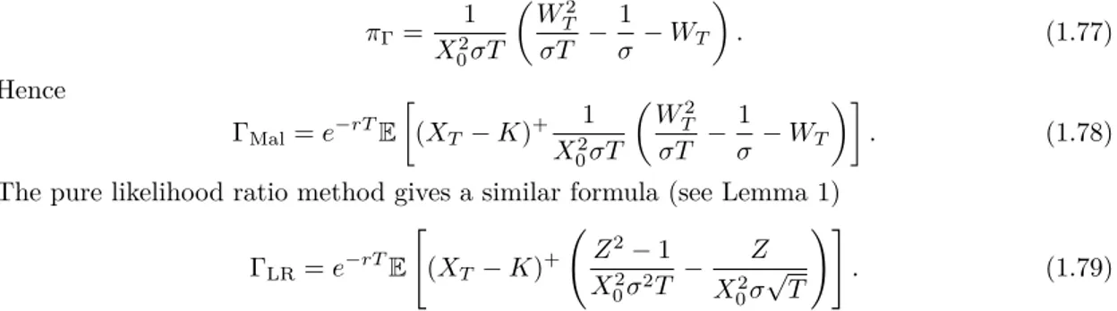
There are also two well known mathematical methods to obtain sensitivities, the so-called log-likelihood ratio method and the Malliavin calculus. However, like the pathwise method, both have their own advantages and drawbacks. For the former, the method consists in differentiating the probability density of the underlying and clearly, it is not possible to compute Greeks if the probability density of the underlying is not known. Yet when the method applies, differentiating the probability density is easy because it is smooth while the payoff may not even be differentiable. More details can be found in Glynn [74], Reiman and Weiss [163], Rubinstein [167] and some applications to finance can be found in Broadie and Glasserman [35] and Glasserman and Zhao [73].
As for the Malliavin calculus, the computation of the Greeks consists in writing the expec-tation of the original payoff function times a specific factor i.e. the Malliavin weight. The main problem is that the computation of the Malliavin weight can be complex and/or computation-ally costly for a high dimensional problem. Several articles deal with the computation of Greeks via Malliavin calculus, Fournié et al. [55], Gobet and Munos [77] and Benhamou [19] to cite a few. The precision of the Malliavin formulas also degenerates for short maturities, especially for ∆-hedging.
Both the likelihood ratio and the Malliavin calculus are generally faster than the finite dif-ference method when the volatility is constant. But implementations of these methods in the financial industry is limited by the specific analysis required for each new payoff.
The chapter is organized as follows; in section 1.2 we begin by recalling Vibrato for first order derivatives as in Giles [60] for the univariate and the multivariate case. We then generalize the method for the second and higher order derivatives with respect to one or several parameters and we describe how Vibrato of Vibrato is identical to analytical or Automatic differentiation of Vibrato.
In section 1.3, we recall briefly the different methods of Automatic differentiation. We describe the direct and the adjoint or reverse mode to differentiate a computer program. We also explain how it can be extended to some non differentiable functions.
Section 1.4 deals with several applications to different derivative securities. We show some results of second order derivatives (Gamma and Vanna) and third order derivatives in the case of a standard European Call option: the sensitivity of the Gamma with respect to changes in the underlying asset and cross-derivatives with respect to spot price and interest rate and others. Also, we compare different techniques of Automatic differentiation and we give some details about our computer implementations. We also illustrate the method on a multidimensional Basket option and on an Autocallable.
In section 1.5, we study the computing time for the evaluation of the Hessian matrix of a standard European Call Option in the Black Scholes model.
In section 1.6 we explain briefly how the computation of the Gamma for an American Put option computed with the Longstaff Schwartz algorithm in Longstaff and Schwartz [124] can be done much in the same fashion as for an European option and on a European Call with Heston’s model in section 1.7.
the context of short maturities. We conclude with a summary and some perspectives for future work.
1.2
Vibrato
Vibrato was introduced by Giles in [60]; it is based on a reformulation of the payoff which is better suited to differentiation. The Monte Carlo path is split into the last time step and its past as represented on the figure 1.1. Let us explain the method on a plain vanilla multi-dimensional option. 0.98 1 1.02 1.04 1.06 1.08 1.1 1.12 1.14 1.16 1.18 0 0.2 0.4 0.6 0.8 1 XT T
Figure 1.1: Representation of Vibrato decomposition on a Monte Carlo path.
First, let us recall the likelihood ratio method for derivatives.
Let the parameter set Θ be a subset of Rp. Let b : Θ× Rd → Rd, σ : Θ× Rd → Rd×q be
continuous functions, locally Lipschitz in the space variable, with linear growth, both uniformly in θ∈ Θ. We omit time as variable in both b and σ only for simplicity. And let (Wt)t≥0 be a
q-dimensional standard Brownian motion defined on a probability space (Ω,A , P).
Lemma 1. (Log-likelihood ratio)
Let p(·, ·) : Θ × Rd 7→ R ,be the probability density of a random variable X(θ); given V ∈
L1(Rd), consider
E[V (X(θ))] = ∫
Rd
V (y)p(θ, y)dy. (1.1)
If θ 7→ p(θ, ·) is differentiable, then, under a standard domination or a uniform integrability assumption, one can interchange differentiation and integration : for i = 1, .., p,
∂ ∂θi [ E[V (X(θ))]]= ∫ Rd V (y)∂ ln p ∂θi (θ, y)p(θ, y)dy =E [ V (X(θ))∂ ln p ∂θi (θ, X(θ)) ] . (1.2)
1.2. Vibrato
1.2.1
Vibrato for a European Contract
Let X = (Xt)t∈[0,T ]be a diffusion process, the strong solution of the following Stochastic
Differ-ential Equation (SDE) {
dXt= b (θ, Xt) dt + σ(θ, Xt)dWt,
X0= x.
(1.3)
Obviously, Xtdepends on θ; for clarity, we write Xt(θ) when the context requires it.
Given an integer n > 0, the Euler scheme with constant step h = Tn, defined below in (1.3),
approximates Xtat time tk= kh, i.e. ¯Xk ≈ Xkh, and it is recursively defined by
{ ¯ Xk= ¯Xk−1+ b(θ, ¯Xk−1)h + σ(θ, ¯Xk−1) √ hZk, k = 1, . . . , n, ¯ X0= x, (1.4)
where{Zk}k=1,..,nare independent random GaussianN (0, Id) vectors. The relation between W
and Z is
Wtk− Wtk−1 =
√
hZk, k = 1, .., n. (1.5)
Vibrato is based on the fundamental remark that if ¯ Xn = µn−1(θ) + νn−1(θ)Zn with Zn independent of µn−1(θ) = ¯Xn−1(θ) + b(θ, ¯Xn−1(θ))h and νn−1(θ) = σ(θ, ¯Xn−1(θ)) √ h, (1.6) then, E[V ( ¯Xn(θ)) ] = E[E[V ( ¯Xn(θ))| (Wtk)k=0,...,n−1 ]] = E[E[V ( ¯Xn(θ))| ¯Xn−1(θ) ]] = E [E [V (µn−1+ νn−1Zn)| µn−1, νn−1]] . (1.7)
This follows from the obvious fact that the Euler scheme defines a Markov chain ( ¯Xk)k=0,...,n
with respect to the filtrationFk = σ(Wtℓ, ℓ = 0, . . . , k).
1.2.2
First Order Vibrato
Let us recall Giles’ result:
Theorem 1. (Vibrato, multidimensional first order case)
∂ ∂θiE[V ( ¯ Xn(θ))] =E [ ∂ ∂θi{E[V (µ n−1(θ) + νn−1(θ)Zn)| µn−1, νn−1]} ] =E [{∂µ ∂θi · E[V (µ + νZn)Σ−1νZn ] + ∂Σ ∂θi :E [ V (µ + νZn) ( −1 2Σ −1+1 2(Σ −1νZ n)(Σ−1νZn)T )] } µ = µn−1(θ) Σ = ννT ν = νn−1(θ) ] . (1.8)
where Σ = hσσT, · denotes the scalar product and : denotes the trace of the product of the matrices.
By ∂θ∂µ
i·E [W (µ, ν, Z)]
µ = µn−1(θ)
nu = νn−1(θ)
we mean that insideE only Z is random, then the result
and ∂θ∂µ
i are evaluated at µn−1(θ), νn−1(θ).
To prove the theorem we set some notations and prove two intermediate results.
We denote φ(µ, ν) =E [V (µ + νZn)]. From (1.7) and (1.3), for any i∈ {1, . . . , p},
∂ ∂θiE[V ( ¯ Xn(θ))] =E [ ∂φ ∂θi ] =E [ ∂µn−1 ∂θi · ∂φ ∂µ+ ∂νn−1 ∂θi : ∂φ ∂ν ] (1.9)
Lemma 2. The θi-tangent process to X, Yt=
∂Xt
∂θi
, is defined as the solution of the following SDE (see Kunita [115] for a proof)
dYt= [ b′θ i(θ, Xt) + b ′ x(θ, Xt)Yt ] dt +[σ′θ i(θ, Xt) + σ ′ x(θ, Xt)Yt ] dWt, Y0= ∂X0 ∂θi (1.10)
where the primes denote standard partial derivatives.
As for ¯Xk in (1.3), we may discretize (1.10) by
¯ Yk+1 = Y¯k+ [ b′θ i(θ, ¯Xk) + b ′ x(θ, ¯Xk) ¯Yk ] h (1.11) +[σ′θ i(θ, ¯Xk) + σ ′ x(θ, ¯Xk) ¯Yk ] √ hZk+1. (1.12) Then from (1.6), ∂µn−1 ∂θi = ¯Yn−1(θ) + h [ b′θi(θ, ¯Xn−1(θ)) + b ′ x(θ, ¯Xn−1(θ)) ¯Yn−1(θ) ] ∂νn−1 ∂θi =(σ′θi(θ, ¯Xn−1(θ)) + σx′(θ, ¯Xn−1(θ)) ¯Yn−1(θ) ) √ h. (1.13)
So far we have shown the following lemma.
Lemma 3. When ¯Xn(θ) is the solution of (1.4), then
∂
∂θiE[V ( ¯
Xn(θ))] is given by (1.9), (1.13)
and (1.11).
In (1.3) b and σ are constant in the time interval (kh, (k + 1)h), therefore the conditional
probability of ¯Xn given ¯Xn−1 is p(x) = 1 (√2π)d√det(Σ)e −1 2(x−µ) TΣ−1(x−µ) (1.14)
where µ and Σ are evaluated at time (n− 1)h and given by (1.6). As in Dwyer and Macphail
[52], ∂ ∂µln p(x) = Σ −1(x− µ), ∂ ∂Σln p(x) =− 1 2Σ −1+1 2Σ −1(x− µ)(x − µ)TΣ−1⇒ ∂ ∂µln p(x)|x= ¯Xn= Σ −1νZ n, ∂ ∂Σln p(x)|x= ¯Xn =− 1 2Σ −1+1 2(Σ −1σZ n)(Σ−1σZn)T
1.2. Vibrato
1.2.3
Antithetic Vibrato
One can expect to improve the above formula – that is, reducing its variance – by the means of an antithetic transform. This can be done on all formulas obtained above. We do it only once, and in the case q = d, to illustrate the methodology. The following holds:
E[V (µ + νZ)ν−TZ]=1
2E
[
(V (µ + νZ)− V (µ − νZ)) ν−TZ]. (1.15)
where ν−T := (νT)−1; similarly, usingE[ZZT − I] = 0,
E[V (µ + νZ)ν−T(ZZT− I)ν−1]
= 1
2E
[
(V (µ + νZ)− 2V (µ) + V (µ − νZ)) ν−T(ZZT − I)ν−1]. (1.16)
Corollary 1. (One dimensional case, d = 1)
∂ ∂θ E[V ( ¯Xn(θ))] = 1 2E [{∂µ ∂θE [ (V (µ + νZ)− V (µ − νZ))Z ν ] + ∂ν ∂θE [ (V (µ + νZ)− 2V (µ) + V (µ − νZ))Z 2− 1 ν ] } µ = µn−1(θ) ν = νn−1(θ) . (1.17)
Remark 1. In the numerical tests, the expectation with respect to Z will be replaced by an
average over MZ paths. For simple cases such as the sensitivities of European options, a small
MZ suffices; this is because there is another average with respect to M in the outer loop, the
number of paths to compute the expectation with respect to µn−1 and νn−1.
1.2.4
Second Order Derivatives
Assume that X0, b and σ depend on two parameters (θ1, θ2) ∈ Θ2. There are two ways to
compute second order derivatives. Either by differentiating the Vibrato (1.8) while using Lemma 1 or by applying the Vibrato idea to the second derivative.
1.2.4.1 Second Order Derivatives by Differentiation of Vibrato
Let us differentiate (1.8) with respect to a second parameter θj:
∂2 ∂θi∂θjE[V (X T)] =E { [( ∂2µ ∂θi∂θj · E [ V (µ + νZ)ν−TZ] +∂µ ∂θi · ∂ ∂θjE [ V (µ + νZ)ν−TZ] ) +1 2 ( ∂2Σ ∂θi∂θj :E[V (µ + νZ)ν−T(ZZT− I)ν−1] + ∂Σ ∂θi : ∂ ∂θjE [ V (µ + νZ)ν−T(ZZT − I)ν−1] )} µ = µν = νnn−1−1(θ)(θ) . (1.18)
The derivatives can be expanded further; for instance in the one dimensional case and after a tedious algebra one obtains:
Theorem 2. (Second Order by Differentiation of Vibrato, d = 1) ∂2 ∂θ2E[V (XT)] =E [{∂2µ ∂θ2E [ V (µ + νZ)Z ν ] + (∂µ ∂θ )2 E [ V (µ + νZ)Z 2− 1 ν2 ] + (∂ν ∂θ )2 E [ V (µ + νZ)Z 4− 5Z2+ 2 ν2 ] +∂ 2ν ∂θ2E [ V (µ + νZ)Z 2− 1 ν ] +2∂µ ∂θ ∂σ ∂θE [ V (µ + νZ)Z 3− 3Z ν2 ] } µ = µn−1(θ) ν = νn−1(θ) . (1.19)
1.2.4.2 Second Order Derivatives by Second Order Vibrato
The same Vibrato strategy can be applied also directly to second derivatives.
As before the derivatives are transferred to the PDE p of XT:
∂2 ∂θi∂θj E[V (XT)] = ∫ Rd V (x) p(x) ∂2p ∂θi∂θj p(x)dx = ∫ Rd V (x)[∂ 2ln p ∂θi∂θj +∂ ln p ∂θi ∂ ln p ∂θj ]p(x)dx =E [ V (x) ( ∂2ln p ∂θi∂θj +∂ ln p ∂θi ∂ ln p ∂θj )] . (1.20) Then ∂2 ∂θ1∂θ2E[V ( ¯ XT(θ1, θ2))] = ∂2φ ∂θ1∂θ2 (µ, ν) = ∂µ ∂θ1 ∂µ ∂θ2 ∂2φ ∂µ2(µ, ν) + ∂ν ∂θ1 ∂ν ∂θ2 ∂2φ ∂ν2(µ, ν) + ∂2µ ∂θ1∂θ2 ∂φ ∂µ(µ, ν) + ∂ 2ν ∂θ1∂θ2 ∂φ ∂ν(µ, ν) + ( ∂µ ∂θ1 ∂ν ∂θ2 + ∂ν ∂θ1 ∂µ ∂θ2 ) ∂2φ ∂µ∂ν(µ, ν),
where µ and ν are evaluated at µn−1, νn−1. We need to calculate the two new terms
∂2 ∂θ1∂θ2 µn−1(θ1, θ2) and ∂ 2 ∂θ1∂θ2
νn−1(θ1, θ2). It requires the computation of the first derivative with respect to θi of
the tangent process Yt, that we denote Y
(2)
t (θ1, θ2).
Then (1.13) is differentiated and an elementary though tedious computations yields the fol-lowing proposition:
Proposition 1. The θi-tangent process Y
(i)
t defined above in Lemma 1.10 has a θj-tangent
process Yt(ij) defined by dYt(ij) = [ b′′θ iθj + b ′′ θi,xY (j) t + b′′θj,xY (i) t + b′′x2Y (i) t Y (j) t + b′xY (ij) t ] dt + [ σ′′θ iθj+ σ ′′ θi,xY (j) t + σ′′θj,xY (i) t + σx′′2Y (i) t Y (j) t + σx′Y (ij) t ] dWt.
Finally in the univariate case θ = θ1= θ2 this gives
Proposition 2. (Second Order Vibrato)
∂2 ∂θ2E[V (XT)] =E [ ∂2µ ∂θ2E [ V (µ + νZ)Z ν ] + (∂µ ∂θ )2 E [ V (µ + νZ)Z 2− 1 ν2 ]
1.2. Vibrato + (∂ν ∂θ )2 E [ V (µ + νZ)Z 4− 5Z2 + 2 ν2 ] +∂ 2 ν ∂θ2E [ V (µ + νZ)Z 2− 1 ν ] +2∂µ ∂θ ∂ν ∂θE [ V (µ + νZ)Z 3− 3Z ν2 ]] . (1.21)
where µ and ν are evaluated at µn−1, νn−1 by 1.6.
Remark 2. It is equivalent to Theorem 2, hence to the direct differentiation of Vibrato.
1.2.4.3 Terms in Vibrato Second Order
Computation of the terms ∂φ
2
∂µ2,
∂φ2 ∂ν2 and
∂φ2
∂µ∂σ. For the second derivative with respect to µ,
we start from ∂φ ∂µ(µ, ν) =E [ V (µ + νZ)Z ν ] = 1 ν2[E[V (µ + νZ)(µ + νZ)] − µE[V (µ + νZ)]] . (1.22) We set ˜ V (µ + νZ) = V (µ + νZ)(µ + νZ). (1.23) Then ∂2 ∂µ2E[V (µ + νZ)] = 1 ν2 [ E [ ˜ V (µ + νZ)Z ν ] − E[V (µ + νZ)] − µE [ V (µ + νZ)Z ν ]] = 1 ν2E [ V (µ + νZ)(µ + νZ− µ)Z ν − V (µ + νZ) ] = E [ V (µ + νZ)Z 2− 1 ν2 ] . (1.24)
Now, for the second derivative with respect to σ, we have (with 1.13, 1.17 and 1.6)):
∂φ ∂σ(µ, ν) =E [ V (µ + νZ)Z 2− 1 ν ] = 1 ν3E[V (µ + νZ)(u − µ) 2]−1 νE[V (µ + νZ)]. (1.25) With ˜ V (u) = V (u)(u− µ)2. (1.26) Hence, ∂2 ∂ν2E[V (µ + νZ)] = 1 σ3hE [ ˜ V (µ + νZ) ( Z2− 1 ν − 3 ν )] −1 νE [ V (µ + νZ) ( Z2− 1 ν − 1 ν )] = E [ ˜ V (µ + νZ)Z 2− 4 ν2 ] − E [ V (µ + νZ)Z 2− 2 ν2 ] = E [ V (µ + νZ)Z 4− 5Z2+ 2 ν2 ] . (1.27)
As for the mixed derivatives with respect to µ then to ν, we have (starting from (1.22) and with ˜ V (µ + νZ) = V (µ + νZ)(µ + νZ),1.13, 1.17 and 1.6) ∂2 ∂ν∂µE[V (µ + νZ)] = 1 ν2E [ ¯ V (µ + νZ) ( Z2− 1 ν − 2 ν )]