Transports et de l’Énergie and Energy
_______________________
Zahabi: Department of Civil Engineering and Applied Mechanics, McGill University, Montreal, Canada
Miranda-Moreno: Corresponding author. Department of Civil Engineering and Applied Mechanics, McGill University, Montreal, Canada. Tel.: 514 398-6589
luis.miranda-moreno@mcgill.ca
Patterson: Department of Geography, Planning and Environment, Concordia University, Montreal, Canada Barla: Centre for Data and Analysis in Transportation (CDAT), Université Laval, Quebec City, Canada
Les cahiers de recherche du CREATE ne font pas l’objet d’un processus d’évaluation par les pairs/CREATE working papers do not undergo a peer review process.
ISSN 1927-5544
Spatio-Temporal Analysis of Car Distance,
Greenhouse Gases and the Effect of Built
Environment : a Latent Class Regression Analysis
Seyed Amir H. Zahabi
Luis Miranda-Moreno
Zachary Patterson
Philippe Barla
Cahier de recherche/Working Paper 2013-1
This work examines the temporal-spatial variations of daily automobile distance traveled and
greenhouse gas emissions (GHGs) and their association with built environment attributes and
household socio-demographics. A GHGs household inventory is determined using link-level
average speeds for a large and representative sample of households in three origin-destination
surveys (1998, 2003 and 2008) in Montreal, Canada. For the emission inventories, different
sources of data are combined including link-level average speeds in the network, vehicle
occupancy levels and fuel consumption characteristics of the vehicle fleet. Built environment
indicators over time such as population density, land use mix and transit accessibility are
generated for each household in each of the three waves. A latent class (LC) regression
modeling framework is then implemented to investigate the association of built environment
and socio-demographics with GHGs and automobile distance traveled. Among other results, it is
found that population density, transit accessibility and land-use mix have small but statistically
significant negative impact on GHGs and car usage. Despite that this is in accordance with past
studies, the estimated elasticities are greater than those reported in the literature for North
American cities. Moreover, different household subpopulations are identified in which the
effect of built environment varies significantly. Also, a reduction of the average GHGs at the
household level is observed over time. According to our estimates, households produced 15%
and 10% more GHGs in 1998 and 2003 respectively, compared to 2008. This reduction is
associated to the improvement of the fuel economy of vehicle fleet and the decrease of
motor-vehicle usage. A strong link is also observed between socio-demographics and the two travel
outcomes. While number of workers is positively associated with car distance and GHGs, low
and medium income households pollute less than high-income households.
Keywords:
Greenhouse gas emissions, spatio-temporal variations, built environment, latent
class regression, household clusters
1. INTRODUCTION
Transportation makes up 27% of Canada’s total greenhouse gas emissions (GHG) - Environment Canada 2010. In addition, transport-related GHGs increased nearly 33% between 1990 and 2005 (Environment Canada 2007). In order to limit climate change, local and worldwide policy makers are looking for strategies to reduce vehicular emissions. In Quebec, the provincial government is aiming to reduce GHG emissions by 20% with respect to 1990 levels by the year 2020.
An extensive literature has developed on different strategies and policy options related to how the built environment (often represented by population density, land use diversity, and transit accessibility) might be used to reduce automobile transportation and transport-related GHG emissions. In this literature, it is contended that planning with the “D’s” in mind will make it possible to reduce automobile dependence by developing dense, diverse, and well-designed neighborhoods with efficient public transportation options. Much of the empirical literature on this topic has found that density, land use and transit accessibility are important factors in determining household travel outcomes such as travel distance and GHGs. The empirical research is typically approached using cross-sectional data. Research using disaggregate data (individual or household level data) is mostly based on cross-sectional analyses comparing mobility patterns across cities or neighborhoods at a single point in time. Moreover, past studies have not studied the potential presence of household subpopulations or classes using a latent class approach. This can help identify whether or not the link between BE and GHGs differs across subpopulations (e.g., certain household subgroups can be more sensitive or react differently to changes in transit accessibility).
As such, the purpose of this research is to estimate the effect of the built-environment on household automobile distance traveled and transport-related GHG emissions, over time and across household subgroups. In order to do this, a unique 3-wave transport related household GHG inventory is built with the Montreal Origin-Destination surveys of 1998, 2003 and 2008. A latent class modeling approach is adopted to determine the differences in built-environment effects across household subgroups.
The paper is structured as follows. The next section contains a literature review. This is followed by a description of the data used, including how the data are combined to develop the household transport-related GHG inventory and built-environment characteristics. Then the modeling framework is described. Input data for the models estimated are summarized and then the empirical results of the statistical models are presented. The final section concludes the paper with policy implications.
2. LITERATURE REVIEW
Due to the size of the literature as well as paper length restrictions, it is not possible to cover the entire literature on the link between travel behavior and the built environment. Instead, this section summarizes the primary literature on the topic, and in particular, the literature considering the effect of built-environment characteristics on vehicle miles traveled (VMT) and GHGs elasticities.
This literature has concentrated on how the built environment, commonly represented by population density, land use diversity, and transit accessibility, might be used to reduce GHGs. In particular, the literature concentrates on whether planning with the “D’s” in mind would make it possible to reduce automobile dependence by developing dense, diverse, and well-designed neighborhoods with efficient public transportation options. Previous literature on travel behavior suggests that density, land use and transit accessibility are contributing factors in determining household travel outcomes such as travel distance and GHGs. For the most part, the literature also agrees that these effects are predictable: higher density, land-use mix and transit accessibility all tend to reduce travel distances and GHG emissions. This literature is so large that there now exist a number of literature reviews on these topics, such as Badoe and
Miller (2000), Handy et al. (2005), Ewing and Cervero (2010) and TRB report 298 (2009). Most of the empirical evidence in this literature is based on cross-sectional studies that have analyzed travel behavior, while controlling for measures of the built environment (BE) and socio-economic control variables. Different statistical approaches and degrees of data aggregation have been used for studying the impacts of built-environment and transit accessibility on travel distance and GHGs. In some studies, the problem of residential self-selection has also been accounted for by using simultaneous equation modeling approaches (Brownstone and Golob (2009), Eluru et al. (2009), Miranda-Moreno et al. (2011)). Also, the relationship between the built environment and travel outcomes has typically been studied at the regional scale using cross-sectional data (Hunter et al. 1990; Donoso et al. 2006; Ewing et al. 2007). Some studies have considered data from several cities (Bento et al. 2003).
Research using disaggregate data (individual or household level data) is mostly based on cross-sectional analyses comparing mobility patterns across cities or neighborhoods at a single point in time. It has been recognized in the literature that if temporal trends are not taken into consideration, built environment – travel outcome relationships may be spurious (TRB report 298, 2009). Moreover, the presence of subpopulations has been demonstrated in other travel outcomes (e.g. Greene and Hensher 2003), but has yet to be explored in the built-environment travel behavior literature. For example, it may happen that car distance and GHGs evolve in different ways across different subgroups, or classes, over time. If subpopulations exist, the effects of built environment factors (density, diversity and transit accessibility) can have different effects on the different groups. Few studies have looked at the temporal and spatial variations of car distance and GHGs across subpopulations in the same region using disaggregate data (household level). The research presented here aims to fill this gap in the literature by estimating the effect of built-environment characteristics on household automobile distance traveled and transport-related GHG emissions over time as well as across subpopulations.
3. DATA USED
As described in more detail in the following section, this research involves calculating household-level, transportation-related GHG emissions, and then estimating the effect of different socio-demographic and built environment characteristics on these emissions. In order to do this, four main types of data are used.
Household-level, transportation-related GHG emissions are estimated from the “bottom-up”, starting with the most disaggregate data possible. The backbone of these calculations is data from three different origin-destination surveys from the years 1998, 2003 and 2008 for the region of Greater Montreal in Canada. The Montreal OD survey is one of the longest running and most detailed in the world. Every five years the survey interviews around 5% of the households in the region (approx. 65,000 households). It is also worth mentioning that this is not a panel dataset – households are selected randomly in each survey. The survey collects information about the households (household structure, number of vehicles, income, etc.), individuals (age, gender, employment status, etc.) as well as detailed information about their travel behavior on the day before the interview. In particular, for each trip by each member of the every household interviewed, the following information is collected: origin and destination locations, transportation mode(s), purpose, transit lines used, time of departure, car occupancy, etc. The socio-demographic information provided by these surveys is also used in the statistical models estimated to explain these emissions. The OD survey was provided by the regional public transportation planner, the Agence métropolitaine de transport (AMT).
While collecting a great deal of information, the O-D survey does not, however, collect information on the make, model, or year of vehicles owned by each household – something that is crucial to estimating household transportation GHG emissions. As a result, a second dataset is used to infer this information. In particular, information on cars registered by Forward Sortation Area (FSA), the area covered by the first
three digits of a postal code, was obtained from the provincial automobile insurance corporation (the SAAQ). Using this information it was possible to estimate average fuel economy for each household in the region of Montreal.
Critical to the accurate estimation of disaggregate automobile- and bus-related GHGs are travel speeds along links of the road network. Average speeds for every link of the road network for the three different years of the OD survey were obtained from the provincial ministry of transportation. These link speeds resulted from the ministry’s EMME-based transportation model. For commuter-rail transportation, diesel fuel consumption was provided by the AMT.
The final element used to explain transport-related GHG emissions are built-environment characteristics. As described below, the built-environment is characterized by three different variables. First, population density is derived from the most recent Canadian census of the population before a given OD survey year (i.e. 1996, 2001 and 2003). Second, transit route stops and frequencies were provided by the AMT. Finally, land-use classifications were obtained from the product CanMap Route Logistics from DMTI Spatial, a company specializing in geographic data related to road networks and land-use.
4. METHODOLOGY
The purpose of this research is fundamentally the calculation of household-level, transportation-related GHG emissions, and then the estimation of the effect of different socio-demographic, and particularly, built environment characteristics on these emissions. This is accomplished in four steps: i) the calculation of trip-level GHGs; ii) the calculation of built-environment characteristics; iii) the estimation of the effect of built-environment characteristics on distance traveled and transport-related GHG emissions, over years and across population subgroups; and iv) finally the comparison across years of the elasticities of built-environment and socio-demographic characteristics on car-distance driven and transport-related GHG emissions. Each of these methodological steps is described in order in the rest of this section.
4.1.
Trip-Level GHGs:
For each trip in the three O-D surveys (1998, 2003 and 2008), two GHG emitting mode categories are distinguished; private motor vehicles, and public transit including transit buses and commuter trains. Some trips can involve more than one mode. The procedure for GHG emissions estimation is described as follows:
i. From a traffic assignment model developed and calibrated by the Quebec provincial ministry of transportation (MTQ) (Babin 2006), congested times for each link of the road network were obtained along with their distances. Link travel times were obtained hourly for all periods of the day.
ii. Each trip was associated (according to its departure time) to a particular (time-of-day) network described in the previous step. The shortest path (based on congested times) was then calculated for each trip to obtain route, link distances and speeds for each link.
iii. For each trip and each emitting mode, ridership, fuel consumption rates and emission factors were calculated
iv. Overall GHG emissions for each trip were then calculated according to equations 1 and 2 below.
For trips involving motor vehicle as a unique or combined mode, the emissions are estimated using distance and average speed at the link level, vehicle fuel consumption rate (FCR) at the FSA-level and GHG emission factors. This procedure is detailed in Barla, et al. (2009) and Barla, et al. (2011). Then, emissions for a given trip j departing in a particular hour t is estimated as:
(1)
Where:
A – automobile
i – Link (i=1,…, N links used by trip j) j – Trip
t – Departure time (hour)
GHGAjit = GHGs for automobile trip j (in kg of CO2) departing at time t.
Dij = Travel distance on segment (link in network) i in 100km.
SPijt = Speed correction factor for segment i of trip j departing at t. Since fuel consumption also depends
upon speed, speed correction factors developed by the MTQ were also used. These factors were produced after a local calibration of MOBILE6 (for further details, see Babin et al. 2004). Link speed was matched with its corresponding speed correction factor.
FCAj = Average fuel consumption rate (FCR) in liters of gasoline/100km for the vehicle used in trip j. This
was generated using the motor-vehicle fleet inventory of the automobile insurance corporation of Quebec (SAAQ). For further details see (Barla et al. 2008). This inventory contains the make, year and model of each vehicle in the province as well as the fuel consumption rate per km. However, the address of the vehicle is provided at the FSA (3-digit postal code). Therefore, FCR at the FSA were generated. An FCR is then associated to each vehicle belonging to the same FSA.
EFA = Emission factor for gasoline (2.289 kg of CO2/ liter of gasoline). This is obtained from the national
inventory report by Environment Canada. 2 Although this number is fixed for all gasoline vehicles for CO2,
for other GHG emissions such as CH4 and N2O, the emission factor depends on the type of vehicle (e.g.
Light duty, heavy duty, Oxidation Catalyst, non-catalytic controlled and etc.). Since we didn’t have knowledge of the type of vehicle owned by the household, we were unable to estimate the emission for other GHG emissions.
RAj = Number of passengers in trip j including the driver. This is determined from the O-D survey data.
Car trips in the same household, departing at the same hour and with the same origin-destination are associated to the same motor-vehicle trip.
For uni-modal or multimodal trips involving public bus transit and/or commuter trains, GHGs are estimated in a similar fashion. In this case, however, average speeds at the trip-level are used since link-level speeds were not available, but this speed estimate considers congestion. For the bus portion, GHGs are calculated using the following equation:
Bj B Bj Bj Bj
R
EF
D
)
S
(
FC
GHG
(2)GHGBj = GHGs for bus portion of transit trip j (kg of CO2)
FC(S)B = Average fuel consumption as a function of operating speeds (S) in liters of diesel/100km).
2
National Inventory Report 1990-2009 (2011 submission), Environment Canada. (http://www.ec.gc.ca/ges-ghg/default.asp?lang=En&n=AC2B7641-1) Aj A Aj N 1 i ijt Aij Ajt R EF FC ] D SP [ GHG
Fuel consumption rates for the typical fuel bus technology operating in real conditions were obtained from a recent field study done by the local transit agency, the Société de transport de Montréal (STM). The fuel
consumption curve according to this study is given by FC(S) = 255.33*(Bus speed) -0.4753
DBj = Distance traveled by bus in transit trip j (km). For each trip involving transit (bus, metro and
commuter trains) in the Montréal region, distances are obtained using the public transit software, MADIGAS (Chapleau 1992). Trips were simulated by the Agence Métropolitaine de Transport (AMT).
EFB= Emission factor for diesel. Here, an emission factor of 2.663 kg CO2/ liter of diesel is considered
based on the recommendation of Environment Canada for Canadian city conditions2.
RBj= Ridership for bus on trip j. In this case we use a mean value for each line used in the trip. This is
obtained from the bus provider agencies for each bus line.
For commuter train lines using diesel or diesel-electric locomotives, average fuel consumption for passenger-km (FC/PK) were directly estimated by the local commuter train agency (Agence métropolitaine de transport - AMT). This was done by dividing the annual fuel consumption (liters of diesel) by their respective annual passenger kilometers traveled. Travel distance by rail (DR) is then estimated for each trip (km). By multiplying (DR) by the fuel consumption rate per passenger km (FC/PK), liters of fuel consumed for the train segment are estimated. To get the kg of CO2 for each trip, the
resulting liters of fuel for each trip is multiplied by the emission factor for CO2 obtained from
Environment Canada. This is equal to 2.663 kg of CO2 for each liter of diesel fuel consumed by trains.
The GHG emissions from the metro (subway system) are assumed to be zero since it runs on hydro-electricity.
To obtain the household inventory, GHGs are estimated for each uni-modal and multimodal trip in the O-D surveys. Trip level emissions are then aggregated at the individual and household level.
4.2.
Calculation of Built-environment Characteristics
To generate the BE indicators in the vicinity of each household involved in this analysis, a nine-cell grid approach was undertaken (Miranda-Moreno et al. 2011). This is done in order to keep the benefits of a region-wide grid but to partly overcome the inaccuracies (the instability of the results) in a normal grid method. The approach involves creating a 500m x 500m grid for the Montreal census metropolitan area (CMA). To calculate the indicators of each cell, the attributes of the eight surrounding cells are considered equally and applied to this central cell. In defining a grid cell at 500 meters, the nine-cell grid method creates an area that approximates a buffer with an approximately 900 m radius (the minimum “radius” is 750 m, and the maximum is 1061 m) – for details see Miranda-Moreno et al. 2011.
According to this grid approach, the following indicators are built for each year involved in the analysis (1998, 2003, and 2008):
Land use mix: Using the nine-cell grid approach, land use mix was calculated using the entropy index (Theil et al. 1971; Frank et al. 2005). The land uses considered are those defined by Desktop Mapping Technologies Inc. (DMTI) which include residential, commercial, institutional and governmental, resource and industrial, and park and recreation, with water and open area not being considered. The computation of this index is according to the common equation that can be seen in Frank et al. (2005) and Miranda-Moreno et al. (2011).
Population density: Population was obtained at the census tract level from Statistics Canada for the Montreal CMA. Land use data from DMTI Spatial was then used to more accurately allocate
population within each census tract, which then allowed for the calculation of approximate population per grid cell.
Transit accessibility: The grid approach was also used to calculate accessibility to transit by finding the nearest bus, metro and rail line stops to each cell and summing each line’s closest stop’s contribution to a transit accessibility index; a stop closer to a cell centroid or with a smaller headway (calculated using AM peak) would mean a larger contribution to transit accessibility. This is calculated as: PTm k 1
n 1
k [d h ]
, where PTm denotes accessibility to public transitat cell m, d stands for distance, in km, from cell centroid m to nearest bus stop of line k (minimum value of 0.1 km) and h stands for average headway, in hours, of line k in AM peak (maximum value of 1 hour).
Note that these three indicators have been used in our previous research. Other BE indicators can be included (e.g. employment density); however, high correlation with these three indicators became an issue. Moreover, it is important to mention that the value of these indicators evolves over time across the three time periods.
4.3.
Modeling Approach Adopted
To estimate the effect of BE and socio-demographics on GHGs, first a traditional OLS approach is adopted and is then contrasted with the results of Latent Class (LC) regression (Vermunt and Magidson 2005). For model definition, consider J homogenous classes of households, with j=(1,…, J) where J is to be defined as part of the calibration process. Then, within each class, we represent the GHGs outcomes using a log-linear model with fixed temporal effects for the years, with i representing a household (i=1,…, n). Then equation 3 represents the log-linear GHGs produced by household i belonging to the class j (j=1,…, J):
( ) (3) Where:
ln(GHGij)= natural logarithm of GHGs for household i which belongs to class j
= model parameters specific to regression model of class j = socio-demographics of household i affecting household i GHGs
= BE attributes (population density, entropy and PT accessibility) in the vicinity of i
= year fixed effect (the year of the OD the household data belongs to), with t being a dummy variables = random independent error term, normally (Gaussian) distributed for household i and class j
Now to assign households to classes, the multinomial logit structure is used for the household segmentation model. The regression function for assigning a household i to class j is defined as:
(4) where is a vector of household attributes that influences the propensity of belonging to class j. Also, is the corresponding vector of coefficients and is the random error term assumed to be identically and independently distributed (with a Type 1 Extreme Valued error). Then, the probability that household i belongs to class j is determined by:
Then, the unconditional probability of GHG emissions production at household i is given as | ∑ | . In order to define the optimal number of classes, different numbers of classes are tested for the same model. The number of classes for the model with the lowest BIC (Bayesian Information Criterion) is selected. In LC regression the special case of 1-class corresponds to the homogeneous population assumption made in traditional regression – which means that population is not segmented. Moreover, the regression parameters are estimated simultaneously for classes and GHGs equations. The estimation is performed in LatentGold software (version 4.5).
5. DATA
This section describes the input data used in the latent class modeling. As described in section 3, the main data components are O-D surveys, BE data and fuel consumption rates for the Montreal motor vehicle fleet.
O-D Survey Data: A summary of the main household-level socio-demographic characteristics obtained from each O-D survey is provided in Table 1. Note that numbers are more or less consistent over time. However, some variations are observed, such as the decrease in the number of children and students. It is also important to mention that in order to make the three waves comparable in terms of area covered, the O-D survey region of the survey 1998 was used as the reference region. Then, households of the O-Ds 2003 and 2008 located outside the 1998 O-D survey were excluded. Moreover, trips with destinations outside of region were considered; however, only the emissions associated to the part of the trip done in the region were included in the inventory.
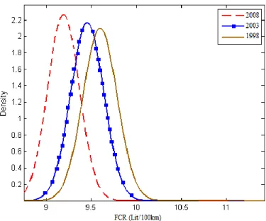
Vehicle Fleet Inventory: The original data from the Quebec provincial vehicle inventory comes from the provincial automobile insurance corporation, the SAAQ. This data was then treated by CDAT (Centre for Data and Analysis in Transportation-Laval University) in order to obtain fuel consumption rates according to the make, year and model. The distribution of the FCR across the three waves is shown in Figure 1. It is worth noting that the fuel economy of the fleet increased over the 10 year period. The average FCRs for the years 1998, 2003, and 2008 are 9.57 lit/100km, 9.36 lit/100km, and 9.19 lit/100km, respectively. Built-environment Indicators: Data used for the BE attributes include: (i) Land use shape files that were obtained from Desktop Mapping Technologies Inc. (DMTI) and have been described above; (ii) The population density data come from the Statistics Canada Censuses for the year 1996, 2001 and 2006; (iii) With respect to public transit accessibility, geo-coded transit lines and stops tagged with unique identifiers linking them to weekday AM-peak headways were used. Also, Table 1 shows the summary statistics of the BE indicators in the vicinity of the households across each O-D survey. Note that transit accessibility and population density increase over time. Unsurprisingly, land-use mix stays very stable. The maps in
Figure 2 show population density, land use mix and transit accessibility, in Montreal for the year 2003.
For the other years of O-D surveys (1998 and 2008) similar maps have been generated, but not reported here due to lack of space. Each household is assigned a value for each of these indicators based on the grid cell in which their dwelling is located and the year of O-D survey in which they were observed.
6.
RESULTS
This section starts by introducing the emission inventory results. Then, the outcomes of the LC model are provided with a discussion
6.1.
Household travel distance and emission inventory
Summary statistics of travel distances and emissions at the household level are presented in Table 2. From this, one can see that both the distance and GHG emissions have decreased across the three periods.
Figure 1 shows the distribution of the fuel consumption rates in the region of analysis. From this it can be
seen that FCR has also declined, as a result of the introduction of increasingly fuel efficient cars over the years. As such, a decrease in GHGs is observed, not only as a result of decreasing travel distances but also greener cars (lower FCR).
Figure 3 shows the spatial distribution of GHGs at the household level over the three waves. This map
represents average emissions for total household travel GHGs, for all households falling inside each Census Tract (CT). From this figure it can be seen that the central neighborhoods emit the least, and that the GHG footprint of the households increases towards the suburbs. It is worth mentioning that the exact locations of the household dwellings were not available for the year 2008; instead, the locations were aggregated to the census tract centroid by the agency collecting the OD survey.
6.2.
OLS results
Log-linear (OLS) regression models are presented and compared with estimates reported in the literature. The OLS results are also presented in order to contrast them with the latent class regression estimates obtained for household subgroups. In this first attempt, BE attributes (population density, PT accessibility and land use mix represented by the entropy index) were directly entered in the GHG and distance models as explanatory variables. Natural logarithm of GHG and distance are the dependent variables.
Table 3 presents the results for the two travel outcomes: car usage and GHGs. The regression models
estimated take into account the expansion weights corresponding to each household. From this table, we can see that BE variables (population density, PT accessibility and LU mix) are statistically significant and negatively associated to both household travel GHGs and distance traveled. From the elasticities, one also can observe that increasing population density and PT accessibility by 10% (one at a time) would reduce household GHGs by 2.08% and 1.56%, respectively, and would reduce distance traveled by 2.20% and 2.12% respectively. For land use mix, elasticities are slightly higher, -2.97% and -3.64 for GHGs and distance respectively - for a 10% increase in the entropy index. Despite that elasticities for distance are slightly higher than for GHGs, the results are consistent for both outcomes. This is in accordance with the literature, in terms of sign and significance; however, the magnitude of these parameters seems to be slightly greater than most of the past studies reported in the literature for North American cities. This may be linked to the fact that the Montreal region has a higher population density and better transit supply than many US cities on which past studies are based. For instance, a recent literature review by the
transportation research board (TRB) (2009) reported elasticities of between -0.1 and -0.24 for car distance traveled with respect to residential density (i.e. an increase of 10% in residential density causes a
reduction of 1 to 2.4% in trip distance). Also, the TRB study found that the elasticity for land use mix (entropy) is 0.5% for a 10% increase in entropy. As for accessibility, the same study reports a 2% increase for a 10% increase in accessibility. In a more recent study, Ewing and Cervero (2010) conducted a meta-analysis on the built environment-travel literature before 2009 for different travel outcomes (VMT, walking, and transit use). They found that a 10% increase in population density causes 0.4% reductions in VMT. Also by increasing land use mix (entropy index) by 10%, trip VMT is found to go down by 0.9%. For transit accessibility, this study reported an average weighted elasticity of -0.05. More recently, Barla et al (2011) reported that a 10% higher residential density would result in 2% decrease in emissions. In most of the cases, reported elasticities are slightly lower than those reported in this study.
Another interesting result is obtained from the fixed effects for the year of the O-D surveys. The positive, yet decreasing, elasticities for these fixed effects suggest that both emissions and distance traveled have a declining trend over the 10 year period. More precisely, household GHGs for 1998 and 2003 are 15% and 10% higher than 2008, respectively. Distance is 15.8% and 24.7% higher than 2008 for 2003 and 1998, respectively. Since GHGs have been decreasing at a faster rate than distances, the decrease in emissions appears partly explained by better fuel economy of the automobile fleet over the 10 year period (Figure
1).
With respect to employment, different employment status variables are statistically significant. Increasing the number of full time workers by one unit increases total household GHG emissions and distanced traveled by 51% and 62%, respectively. Increasing the number of part time workers increases household GHG emissions and distance traveled by 31% and 38%, respectively.). This shows the important link between labor force participation and transportation-related GHGs and distance traveled at the household level. The single adult family variable (household with only one member whom is an adult) is also found to be statistically significant. This type of household has a much smaller (32% less in model 1 and 45% in model 2) carbon footprint and distance traveled comparing to households with more than one member. The presence of retirees in a household reduces only slightly the household GHGs.
6.3.
Latent class results
For the selection of the best number of classes (subgroups) in the LC regression analysis, different numbers of clusters were attempted. The BIC values were then used as a goodness of fit (selection) criterion. The aim was to identify the model with the lowest BIC and with a reasonable number of observations in each class. Also, for the regression models (for both GHG and classes equations) different combinations of variables were tested. Particular attention was paid to avoid high correlation among explanatory variables. The regression models take into account the expansion weights corresponding to each household. After trying different numbers of sub-groups (classes) and variable combinations, a 3-class model was selected and reported in Table 4. In the GHG model results, in addition to the built environment variables (population density, land use mix and transit accessibility), several socio-demographic and year fixed effects are statistically significant. In the class model, three variables were retained as covariates to assign households to classes. These are the number of cars, number of children, and household size (number of persons in the household), and are also reported in the second part of
Table 4.
The following observations can be made about the three classes:
Class 1 has the lowest car ownership, number of children and people among the 3 classes. It
mainly consists of households on the island of Montreal (84%) and towards central areas.
Class 2 has intermediate values for these attributes (higher than class 1 but lower than class 3) and
is mostly located between the other two mentioned classes geographically.
Class 3 has the highest value for these attributes (the highest number of cars, children and people)
and is mostly located outside the island of Montreal in suburbs.
For each class, the GHG regression model parameters are presented in Table 4. Also, the multinomial logit outcomes are presented at the end of this table. Among other results, it is observed that:
The three built environment factors are found to be significant at 0.05 significance levels. As in the previous OLS models, BE attributes have a negative effect on both GHGs and car usage.
More importantly, the size of the parameters is statistically different across household types (by comparing coefficients of classes 1 to 3). This confirms that the effectiveness of built environment policies may vary significantly across household classes. This also shows the importance of segmenting the household population in subgroups with different dynamics over time.
The effects of population density and entropy (LU mix) are the highest for households in class 3. For instance, the impact of density on distance traveled is -1.32 % and -1.7% for GHGs. Note that households on this subgroup are located mainly on the peripheries, with lower density and LU mix. This means that they have more potential for increases in density and entropy. It is worth mentioning that population density variables per year were also tested but since the coefficients were close this model was not reported.
For PT accessibility, households in class 2 and 3 present very similar elasticities for both GHGs and distance. They are also significantly higher than households in subgroup 1. As was the case for entropy and population density, this suggests that these household classes can react differently to transit improvement strategies than households in central areas.
From the yearly fixed-effects, one can see different trends for each class type. For households in classes 2 and 3, the emissions are significantly higher in 1998 and 2003 with respect to 2008. A similar decrease over the years in car distance travelled is observed.
However, GHGs in class 1 show an inverse effect; GHG emissions increased over time despite a decrease in distance travelled. As mentioned before, class 1 is mainly located in central neighborhoods with the lowest values for car ownership. To identify the cause, the fuel consumption and travel speeds affecting emissions were analyzed further. For this, we plotted the FCR (fuel consumption rate) histograms of each class for each OD year. Despite that the overall FCR for the region has declined over time, in this subpopulation of households the FCR is increasing across the 3 waves. This could be associated to different factors. For instance, households belonging to this class may tend to keep their motor vehicles over longer time periods or these households are getting bigger cars (less fuel-efficient cars). Gentrification has been bringing wealthier people downtown and in rich central neighborhoods. One interesting future research could be to look at sport utility vehicles (SUV) penetration.
Moreover, employment status of the household plays an important role in car usage and emissions. By adding one full time and part time worker to the household, there is an average increase of 36% and 16.6%, respectively, in GHGs in class 2. The single adult family variable has a smaller (e.g., 13% less in model 3 for class 3, and 59% less in model 4 for class 3) carbon footprint and car distance comparing to households with more than one member. Income also plays an important role in the carbon footprint with low and middle class households having less contribution compared to the high income class households. This is as much as 32% less GHGs and 28% lower car distances in the low income class households.
7. CONCLUSIONS
This research investigated the effect of built environment characteristics on GHGs and automobile distance traveled at the household level in the region of Montreal, Canada. For this purpose, a GHG inventory was first determined for each household participating in the O-D surveys for 1998, 2003, and 2008. A temporal and spatial exploratory analysis was then implemented. This is followed by a latent-class regression analysis that segments the dataset into household subgroups (latent-classes) and helps improve the goodness-of-fit. Among other results, it was found that land use mix, population density and public transit accessibility have statistically significant and negative effects on household GHGs and car distance travel. This is in accordance with the literature; however, the elasticities obtained in this study are greater than those obtained in past studies involving US & Canadian cities. Moreover, our results demonstrate that the effects of built environment can vary considerably across
subgroups (household
subpopulations). This suggests that different household subgroups can respond differently to changes in the builtenvironment. For instance, an increase in public transit accessibility in the subgroups of households located out of central neighborhoods (classes 2 and 3) is expected to have a greater effect on GHGs than households concentrated in central areas (class 1). This shows the importance of household segmentation through a latent class approach, and how doing so can help indentify specific strategies over the study region.
When looking at the whole household population, it is observed that the average household GHGs have significantly declined during the period of analysis (1998-2008). This reduction can be associated to both the reduction in car usage (car distance) as well the improvement of the global fuel efficiency of the fleet over the ten-year period of analysis. However, when looking at different population classes, it is observed that for the subgroup of households concentrated in central neighborhoods and characterized by a lower car ownership, GHGs are growing over the three waves. This may be due to the fact that the motor-vehicle fleet in this subgroup has been aging, meaning that fuel efficiency is not improving. Again, this highlights the importance of looking at household subpopulations which, as demonstrated here, can have different dynamics over time (trends).
Among the socio-demographic variables, employment status and income are also significantly related to household GHG emissions; having more workers in the household and a higher income adds to the GHGs contribution and car travel distance. This shows that a large share of GHGs is due to daily commuting. This highlights the importance of strategies to target commuting motor-vehicle trips and high income households. Households with retirees are only generating slightly less GHGs. This suggests that the aging of the population will not necessary produce a significant reduction in fuel consumption.
This study highlights the importance of taking into account the spatial and temporal variations in the identification of initiatives to reduce the carbon footprint of households in a region. In the formulation of policies and scenarios, not only built environment and socio-demographics factors should be taken into account, but also the evolution of the fuel efficiency of the motor-vehicle fleet. A significant reduction in car usage along with a significant improvement of the motor-vehicle fuel efficiency of the Montreal’s fleet has been translated in a significant reduction of GHGs at the household level.
Some limitations of this work include the use of fuel consumption rates at the zonal (FSA) level instead of the household vehicle-specific rates – this was due to the lack of data. As a future work, a vehicle allocation model will be developed to overcome this limitation. Also, a model of dynamic traffic assignment could be implemented to evaluate the impact of estimated speeds.
ACKNOWLEDGMENT
We would like to acknowledge the financial aid provided by FQRNT under the program “recherche en
partenariat contribuant à la réduction et à la séquestration des gaz à effet de serre”. We would like also
to thank the “Agence métropolitaine de transport - AMT” and “Transports Québec – MTQ” for providing technical support and data – in particular O-D surveys and road/transit networks.
REFERENCES
Babin, A., P. Fournier, & L. Gourvil (2004). Modèle d’émission des polluants et des GES et modèle de consommation des carburants pour MOTREM, Service de la modélisation des systèmes de transport, Ministère des Transports du Québec, 221.
Babin. A. (2006). Modèle exploratoire sur l’utilisation du réseau routier à l’échelle du Québec. Bibliothèque nationale du Québec.
Badoe, D. & E. Miller. (2000). Transportation—Land Use Interaction: Empirical Findings in North America, and their Implications for Modeling. Transportation Research Part D, Vol. 5, No. 4.
Barla, P., Miranda-Moreno, L.F., Savard-Duquet N. & M. Lee-Gosselin (2008). Analysis of the determinants of the energy efficiency of new light vehicles in Quebec from 2003 to 2008, CDAT.
Barla, P., Lamonde, B., Miranda-Moreno & L.F., N. Boucher (2009). Traveled Distance, Stock and Fuel Efficiency of Private Vehicles in Canada: Price Elasticities and Rebound Effect, Transportation , vol. 36, no 4, pp. 367-467
Barla, P., Miranda-Moreno, L.F. & M. Lee-Gosselin (2011). Urban Travel CO2 Emissions and Land Use: a Case Study for Quebec City, Transportation Research Part D: Transport and Environment.
Bento, A. M., Cropper, M. L., Mobarak, A. M., & Vinha, K. (2003). The impact of urban spatial structure on travel demand in the United States. (World Bank policy research working paper #3007).
Brownstone, D., & Golob, T. F. (2009). The impact of residential density on vehicle usage and energy consumption. Journal of Urban Economics, 65(1), 91-98.
Cao, X., P. Mokhtarian, & S. Handy. (2008). Examining the Impacts of Residential Self- Selection on Travel Behavior: Methodologies and Empirical Findings. Research Report UCD-ITS-RR-08-25. Institute of Transportation Studies, University of California, Davis.
http://pubs.its.ucdavis.edu/publication_detail.php?id=1194. Accessed on March 30, 2009.
Chapleau, R. (1992). La modélisation de la demande de transport urbain avec une approche totalement désagrégée. In Proceedings of the 6th World Conference on Transportation Research, Lyon, France.
Donoso P., Martínez F. & Zegras C. (2006). The Kyoto Protocol and Sustainable Cities: The Potential Use of the Clean Development Mechanism in Structuring Cities for “Carbon-Efficient” Transport. Transportation Research Record 1983: 158-166.
Eluru, N., Bhat, C., Pendyala, R., & Konduri, K. (2009). A Joint Flexible Econometric Model System of Household Residential Location and Vehicle Fleet Composition/Usage Choices. Springer Science + Business Media.
Environment Canada (2007). Greenhouse Gas Division. National Inventory Report 1990-2005:
Greenhouse Gas Sources and Sinks in Canada. Ottawa, Environment Canada (Cat. No. En81-4/2005E,
Table 3-4).
Environnent Canada (2010). Environnent Canada's Online Newsmagazine. Issue 100, Taming Transport: New Regulations for Greenhouse.
http://www.ec.gc.ca/envirozine/default.asp?lang=En&n=AB656AC7-1
Ewing, R, Bartholemew, K., Winkelman, S, Walters, J & Chen, D (2007). Growing Cooler: The Evidence on Urban Development and Climate Change. Urban Land Institute:Washington DC.
Ewing, R., & Cervero, R. (2010). Travel and the Built Environment: A Meta-Analysis. Journal of the American Planning Association 76 (3): 265–94.
Frank, L. D., Schmid, T. L., Sallis, J. F., Chapman, J., & Saelens, B. E. (2005). Linking objectively measured physical activity with objectively measured urban form: Findings from SMARTRAQ. American Journal of Preventive Medicine, 28(2, Supplement 2), 117-125.
Gim. T-H. T. (2011). A meta-analysis of the relationship between density and travel behavior. Transportation, Volume 39, Issue 3, pp 491-5
Greene, W. H., & D. A. Hensher. (2003). A Latent Class Model for discrete choice analysis: contrasts with mixed logit. Transportation Research Part B: Methodological, Vol. 37, No. 8, pp. 681–698.
Handy, S. (2005). Smart Growth and the Transportation-Land Use Connection: What Does the Research Tell Us? International Regional Science Review, Vol. 28, No. 2, pp. 146–167.
Hunter, John E., & Frank L. Schmidt. (1990). Methods of Meta-analysis: Correcting Error and Bias in Research Findings. Newbury Park: Sage Publications.
MDDEP (2007). Ministère du Développement durable, de l'Environnement et des Parcs du Québec.
Miranda-Moreno, L., Bettex, L., Zahabi A., Kreider, T. & Barla P. (2011). A simultaneous modeling approach to evaluate the endogenous influence of urban form and public transit accessibility on distance traveled, Journal of Transportation Research Record Vol. 2255, pp 100-109.
Statistics Canada. 2001 and 2006 Census of Population, Montréal (862 areas). E-STAT (distributor).
Theil, H., & Finizza, A. J. (1971). A note on the measurement of racial integration of schools by means of informational concepts. Journal of Mathematical Sociology, 1(2), 187-193.
TRB-Transportation Research Board (2009) Driving and the Built Environment: The Effects of Compact Development on Motorized Travel, Energy Use, and CO2 Emissions, Special Report 298, Washington DC, National Research Council.
Vermunt J.K. & Magidson J. (2005). Technical Guide for Latent GOLD 4.0: Basic and Advanced. Belmont Massachusetts: Statistical Innovations Inc.
Category Variable Mean 1998 Std. Dev 1998 Mean 2003 Std. Dev 2003 Mean 2008 Std. Dev 2008 Socio-demo Number of cars 1.29 0.86 1.20 0.91 1.24 1.02 Number of persons 2.56 1.31 2.33 1.27 2.33 1.29
Number of children (younger than 15) 0.60 0.96 0.45 0.85 0.50 0.89
Number of full time workers 1.13 0.82 1.02 0.84 0.97 0.87
Number of part time workers 0.13 0.36 0.11 0.33 0.11 0.33
Number of students 0.64 0.95 0.56 0.91 0.53 0.89
Number of retirees 0.27 0.58 0.32 0.61 0.42 0.67
BE
Population density * (people per hectare) 42.77 31.91 47.04 34.36 47.57 34.30
Transit accessibility * 108.48 119.00 120.87 126.44 121.43 123.85
Land use mix (entropy)* 0.32 0.16 0.34 0.17 0.34 0.17
Variable 1998 2003 2008
Average total GHG (kg/day)* 10.70 10.32 10.02
Average car GHG (kg/day) * 10.25 10.00 9.61
Average total distance at household (km/day) * 53.65 51.08 47.82
Average car distance at household (km/day) * 45.23 43.68 39.66
Number of households in OD survey 53,810 56,959 66,124
Average number of people per car trip 1.26 1.25 1.23
Table 3: OLS model for Ln(household trip GHG) and ln(car distance traveled)
Model 1 –GHG Model 2 – Car distance
Coef. P>|t| Elast % Coef. P>|t| Elast %
Residential density * -0.004 0.00 -2.08 -0.004 0.00 -2.20
PT accessibility * -0.001 0.00 -1.56 -0.001 0.00 -2.12
Entropy * -0.882 0.00 -2.97 -1.083 0.00 -3.64
Year 1998*** 0.140 0.00 15.03 0.146 0.00 15.79
Year 2003*** 0.096 0.00 10.18 0.220 0.00 24.67
Year 2008*** Base case Base case
Number of retirees ** -0.025 0.00 -2.52 -0.016 0.00 -1.67
Number of students ** 0.078 0.00 7.88 0.027 0.00 2.70
Number of part time workers ** 0.311 0.00 31.13 0.385 0.00 38.59
Number of fulltime workers ** 0.510 0.00 51.07 0.621 0.00 62.12
Number of children ** 0.012 0.00 1.27 0.075 0.00 7.57
Single adult family*** -0.385 0.00 -31.98 -0.604 0.00 -45.39
Low income (less than 40k)*** -0.557 0.00 -42.72 -0.629 0.00 -46.73
Medium income (40k to 80k)*** -0.219 0.00 -19.70 -0.205 0.00 -18.57
High income (more than 80k)*** Base case Base case
Constant 2.008 0.00 - 3.041 0.00 -
*(10% increase for elasticity) **(1 unit increase for elasticity) *** dummy variable
Model 3 –GHGs Model 4 – Car distance
Class1+ Elast% Class2+ Elast% Class3+ Elast% Class1+ Elast% Class2+ Elast% Class3+ Elast%
Residential density (in 1000s)* -2.104 -0.95 -2.413 -1.09 -2.902 -1.32 -0.601 -0.27 -1.903 -0.86 -3.705 -1.70
PT accessibility (in 1000s)* -0.101 -0.12 -0.932 -1.05 -0.801 -0.94 -0.303 -0.35 -1.104 -1.30 -1.103 -1.30
Entropy * -0.381 -1.29 -0.540 -1.83 -0.561 -1.93 -0.146 -0.50 -0.639 -2.16 -0.668 -2.30
Year 1998*** -0.256 -22.65 0.339 40.40 0.178 19.52 0.146 15.70 0.415 51.60 0.104 11.00
Year 2003*** -0.182 -16.71 0.224 25.21 0.145 15.73 0.077 8.15 0.364 44.01 0.220 24.60
Year 2008*** Base case Base case
Number of retirees ** 0.079 7.93 -0.229 -22.9 -0.010 -1.02 -0.023 -2.33 -0.161 -16.10 -0.105 -10.60
Number of students ** 0.052 5.27 0.030 3.00 0.077 7.83 -0.003 -0.38 -0.037 -3.71 0.071 7.10
Number of part time workers ** 0.062 6.23 0.166 16.60 0.116 11.63 0.038 3.82 0.164 16.52 0.213 21.30
Number of fulltime workers ** 0.076 7.62 0.362 36.20 0.175 17.55 0.078 7.91 0.322 32.30 0.342 34.20
Number of children ** -0.024 -2.41 -0.107 -10.70 -0.067 -6.76 0.026 2.71 0.105 10.60 -0.056 -5.60
Single adult family*** -0.095 -9.11 -0.094 -9.01 -0.137 -12.83 -0.061 -6.00 -0.203 -18.40 -0.891 -59.00
Low income (less than 40k) -0.062 -6.04 -0.384 -31.90 -0.202 -18.34 -0.045 -4.47 -0.194 -17.60 -0.333 -28.40
Medium income (40k to 80k) -0.025 -2.56 -0.145 -13.56 -0.094 -9.03 -0.008 -0.81 -0.010 -1.04 -0.119 -11.20
High income (more than 80k) Base case Base case
Constant 0.265 - 1.618 - 2.867 - 0.478 - 2.721 - 3.673 -
Multinomial model for classes (GHGs) Multinomial model for classes (distance)
Class 1 Class2 Class 3 Class 1 Class2 Class 3
Number of cars -3.650 1.362 2.288 -3.604 1.362 2.283
Number of children -0.272 0.067 0.205 -0.264 0.0671 0.198
Number of persons 0.018 -0.120 0.101 0.019 -0.128 0.106
Constant 2.600 -0.173 -2.427 2.502 -0.163 -2.427
*(10% increase for elasticity) **(1 unit increase for elasticity) *** dummy variable