Precambrian Plate Tectonics in Northern Hudson Bay:
Evidence From P and S Wave Seismic Tomography
and Analysis of Source Side Effects in Relative
Arrival-Time Data Sets
Mitch V. Liddell1 , Ian Bastow1 , Nicholas Rawlinson2 , Fiona Darbyshire3 , Amy Gilligan4 , and Emma Watson1
1Department of Earth Science and Engineering, Imperial College London, London, UK,2Department of Earth Sciences,
University of Cambridge, Cambridge, UK,3GEOTOP Research Centre, Université du Québec à Montréal, Montreal, Canada, 4School of Geosciences, University of Aberdeen, Aberdeen, UK
Abstract
The geology of northern Hudson Bay, Canada, documents more than 2 billion years of history including the assembly of Precambrian and Archean terranes during several Paleoproterozoic orogenies, culminating in the Trans-Hudson Orogen (THO) ∼1.8 Ga. The THO has been hypothesized to be similar in scale and nature to the ongoing Himalaya-Karakoram-Tibetan orogen, but the nature of lithospheric terrane boundaries, including potential plate-scale underthrusting, is poorly understood. To address this problem, we present new P and S wave tomographic models of the mantle seismic structure using data from recent seismograph networks stretching from northern Ontario to Nunavut (60–100∘W and 50–80∘N). The large size of our network requires careful mitigation of the influence of source side structure that contaminates our relative arrival time residuals. Our tomographic models reveal a complicated internal structure in the Archean Churchill plate. However, no seismic wave speed distinction is observed across the Snowbird Tectonic Zone, which bisects the Churchill. The mantle lithosphere in the central region of Hudson Bay is distinct from the THO, indicating potential boundaries of microcontinents and lithospheric blocks between the principal colliders. Slow wave speeds underlie southern Baffin Island, the leading edge of the generally high wave speed Churchill plate. This is interpreted to be Paleoproterozoic material underthrust beneath Baffin Island in a modern-style subduction zone setting.1. Overview
The northern Hudson Bay region in Canada comprises several major Archean (> 2.5 Ga) and Paleoproterozoic domains and collision zones. The region is underlain by a thick (>250 km), high wave speed lithospheric root (e.g., Darbyshire et al., 2013; Porritt et al., 2015) and contains the record of a ∼1.8 Ga continental collision zone, the Trans-Hudson Orogen (THO; e.g., Hoffman, 1988). It is thus an ideal natural laboratory for the study of Precambrian tectonic processes.
Estimates for the onset of modern-style plate tectonics vary from the early Archean to the Proterozoic (e.g., Hawkesworth et al., 2017; Hopkins et al., 2008; Stern, 2005). The early Earth was hotter and more duc-tile, which is thought to have hindered the onset of modern-style plate tectonics (e.g., Stevenson, 2003). However, the apparent stabilization of continental lithosphere and crust ∼3 Ga, as well as the discovery of subduction-related eclogites of a similar age, may point to an Archean emergence of plate tectonics (e.g., Hawkesworth et al., 2017; Tappe et al., 2003). Regardless of when plate tectonics formally began, geological and geophysical consensus is emerging that the Proterozoic THO developed from modern-style plate tec-tonics (e.g., Bastow et al., 2011; St-Onge et al., 2006; Thompson et al., 2010; Weller & St-Onge, 2017). Multiple theories exist regarding the details of THO development, ranging from a relatively simple two-plate orogeny (e.g., St-Onge et al., 2006, 2009) to more complex models including island arc and protocontinent accretion (e.g., Berman et al., 2005; Corrigan et al., 2009; Liddell et al., 2017). Different THO assembly styles may change the way in which geophysical observations are interpreted, since plate tectonic processes can create large lat-eral offsets between the observed surface geology of the crust and mantle lithosphere. Resolving these issues requires an improved understanding of the deep seismic structure of the northern Hudson Bay region. Blocks of distinct composition, inherent since their formation, or as a result of metasomatism, would be expected to
RESEARCH ARTICLE
10.1029/2018JB015473 Key Points:
• Evidence of Precambrian plate-scale underthrusting beneath Baffin Island • Microplates within the Trans-Hudson
Orogen are imaged, complicating the two-plate hypothesis; no seismic distinction at the STZ is observed • Subducting slabs can contaminate
relative arrival time residuals and frequency content; we analyze the effect and show that it may be mitigated Supporting Information: • Supporting Information S1 • Table S1 • Data Set S1 • Data Set S2 Correspondence to: M. V. Liddell, [email protected] Citation:
Liddell, M. V., Bastow, I., Rawlinson, N., Darbyshire, F., Gilligan, A.,
& Watson, E. (2018). Precambrian plate tectonics in Northern Hudson Bay: Evidence fromP andSwave seismic tomography and analysis of source side effects in relative arrival-time data sets. Journal of Geophysical
Research: Solid Earth, 123, 5690–5709.
https://doi.org/10.1029/2018JB015473
Received 11 JAN 2018 Accepted 2 JUN 2018
Accepted article online 9 JUN 2018 Published online 5 JUL 2018
©2018. American Geophysical Union. All Rights Reserved.
manifest as different mantle seismic wave speeds. Underthrust material could manifest as dipping structures or as an extension of wave speed anomalies beneath the overriding region.
The structure of the mantle lithosphere in northern Hudson Bay has previously been constrained by global and regional surface wave models. The Canadian shield was once viewed as a homogeneous fast wave speed block with no distinction between Archean and less-depleted Proterozoic mantle. (e.g., Darbyshire & Eaton, 2010; Ritsema et al., 2011; Shapiro & Ritzwoller, 2002). More recently, models have revealed the THO as a relatively slow band of lithosphere between the Churchill and Superior plates (Figure 1; e.g., Darbyshire et al., 2013). The detailed architecture of this band is unclear, however, due to the relatively poor lateral resolving power of surface waves.
To address outstanding questions about the THO and the internal architecture of the lithosphere beneath northern Hudson Bay, we provide the first dedicated P and S wave tomographic study in the region. Our network comprises 64 seismograph stations distributed around Hudson Bay and the islands to the north (Figure 1). We take particular care to assess the validity of the relative arrival-time method for such a large network. Specifically, we test whether and to what degree the effect of source side structure is removed during the calculation of our relative arrival time residuals.
2. Tectonic Background
The northern Hudson Bay region is dominated by the Superior and Churchill cratons (Figure 1; Hoffman, 1988). The Churchill is divided into the Rae and the Hearne along the Snowbird Tectonic Zone (STZ). The subdi-visions are distinguished geologically by a lack of post 2.66-Ga magmatism in the Hearne (e.g., Davis et al., 2006). Several potential origins of the STZ have been proposed, and the east and west regions may even have different lithospheric structure (Bao & Eaton, 2015). In our study region, the STZ is exposed on the western coast of Hudson Bay and potentially extends to Southampton Island (Spratt et al., 2012). It is characterized by high-pressure metamorphic belts, pointing to a ∼1.9-Ga collision (e.g., Berman et al., 2007). The central Rae craton includes several distinct blocks, suggesting it may also have a complex internal tectonic history (e.g., Skulski et al., 2003).
The THO marks the ∼1.8-Ga collision of Archean domains with the Superior acting as a double indenter into the Churchill (Darbyshire & Eaton, 2010; Gibb, 1983). Other studies have used the term “THO” more broadly to define the entire region of structural and metamorphic overprint due to the collision (e.g., Corrigan et al., 2009). Under this definition the internides of the collision zone itself are defined as the Reindeer Zone. The phys-ical extent of this broader definition includes most of our study region and the entire region of resolution in our inversion models, thus rendering it less useful for our purposes. We therefore use THO in this study to refer to the remains of the collision zone itself and not the wider region of deformation. It is the largest orogen that contributed to the creation of the Paleoproterozoic supercontinent Columbia (Rogers & Santosh, 2002) and is broadly understood to have formed by the closure of the Manikewan Ocean (e.g., Hoffman, 1988; St-Onge et al., 2006, 2009). The THO stretches>4,600 km from central North America to Greenland and is on average ∼500 km wide (St-Onge et al., 2006), although widths of 700 km have been suggested in northern Hudson Bay and Baffin Island (Gilligan et al., 2016; Liddell et al., 2017). The THO developed from a series of smaller oro-genies (see Corrigan et al., 2009, and references therein). The first of these is the 1.92- to 1.89-Ga Snowbird Orogeny, with contemporaneous subduction beneath the western Superior craton; the modern STZ is what remains of this orogeny (e.g., Berman et al., 2007). This was followed by addition of the Meta-Incognita micro-continent and the Sugluk block to the eastern Rae craton (Corrigan et al., 2009). Terminal collision between the Churchill and Superior plate occurred from 1.83 to 1.80 Ga. This was synchronous with significant tectonother-mal reworking, much of which occurred on the weaker, hotter, Churchill province (St-Onge et al., 2006). The THO may have involved a number of smaller microcontinents that were swept up between the larger blocks during ocean closure (e.g., Corrigan et al., 2009). Southern Baffin Island and north-central Hud-son Bay have been postulated to be an amalgamation of some of these microcontinents (Snyder et al., 2013; St-Onge et al., 2006). Recently, high-pressure, low-temperature, eclogite rocks from within the THO have been found by Weller and St-Onge (2017). These are thought to fill a missing link in the geo-logical record in this region and provide compelling evidence for the operation of modern-style plate tectonics by 1.8 Ga.
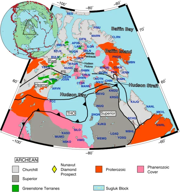
Figure 1. Geological map of Hudson Bay and surrounding areas with Archean material in shades of gray with later
eras in color. Boundaries modified from Corrigan et al. (2009). Circles indicate receiver locations. The inset global map shows the location of the receiver network, the red dots are earthquakes used in this study. Yellow dashed line is the approximate extent of the Sugluk block as defined by Berman et al. (2013). SI=Southampton Island; STZ=Snowbird Tectonic Zone; THO=Trans-Hudson Orogen.
3. Previous Geophysical Studies
Pand S wave global tomographic models reveal fast wave speeds beneath most of North America east of the Rocky Mountains to≥250-km depth (e.g., Lebedev & van der Hilst, 2008; Li et al., 2008; Ritsema et al., 2011; Schaeffer & Lebedev, 2013), but these fast wave speeds are not thought to have resulted in any thermally driven topography on the mantle transition zone (Thompson et al., 2011). The seismic structure of the upper mantle of the western Superior province was constrained with P and S wave models by Sol et al. (2002). The authors found evidence for a ∼300-km-thick cratonic root and interpreted a deep high-velocity anomaly as a remnant Archean-age subducted slab. Further work on the Superior province by Frederiksen et al. (2007, 2013) found a significant change in lithospheric mantle character between the west and east Superior and imaged the mantle expression of the Superior/Trans-Hudson contact. These were both significant mantle velocity signatures that were unconnected to crustal expressions. Continent-wide receiver function results (e.g., Abt et al., 2010), and long-period waveform inversion (e.g., Yuan & Romanowicz, 2010; Yuan et al., 2011), have contributed to a picture of a continent-scale two-layer lithospheric model. North America is thought to
have grown episodically, with a chemically depleted upper ∼150–200 km underlain by younger, less depleted material. This change may be distinguished by a change in anisotropic fast direction (e.g., Darbyshire et al., 2013; Liddell et al., 2017; Petrescu et al., 2017). Sharp discontinuities imaged at midlithospheric depths by receiver function studies throughout cratonic North America (Abt et al., 2010) and within northern Hudson Bay have supported this episodic growth theory (e.g., Porritt et al., 2015; Rychert & Shearer, 2009).
The UK Hudson Bay Lithospheric Experiment (e.g., Bastow et al., 2015) involved seismometers installed on the northern islands of the Hudson Strait and Baffin Island, complementing the existing POLARIS network (Eaton et al., 2005) and increasing the resolution in the northern part of the Bay dramatically. These, in combination with other seismograph networks, have been used to provide improved insight into the crustal structure (e.g., Gilligan et al., 2016; Pawlak et al., 2011, 2012; Thompson et al., 2010, 2015), mantle wave speed (e.g., Darbyshire et al., 2013), and mantle anisotropy (e.g., Bastow et al., 2011; Liddell et al., 2017; Snyder et al., 2013). Based on two-station path-averaged Rayleigh wave dispersion analysis, Darbyshire and Eaton (2010) found no seismic wave speed distinction between Archean and Proterozoic mantle. However, anisotropic surface wave tomo-graphic models from Darbyshire et al. (2013) resolved slower Proterozoic material associated with the THO between the faster Archean Superior and Churchill cratons; they also estimated a Lithosphere-Asthenosphere Boundary (LAB) depth of ∼250 km beneath the Bay and surrounding areas using a 1.7% fast shear veloc-ity contour as a LAB proxy. Receiver function results from Porritt et al. (2015) showed an exceptionally thick lithosphere (∼350 km) beneath central Hudson Bay and widespread midlithospheric discontinuities. SKS splitting results by Bastow et al. (2011) showed that anisotropic fast directions were, to first order, con-trolled by the nearby THO, and variable anisotropic splitting parameters on Baffin Island were interpreted as being due to a potential dipping layer. A larger scale study by Snyder et al. (2013) observed widespread anisotropic patterns indicative of multiple layers. Most recently, Liddell et al. (2017) used forward modeling to characterize the nature of regional anisotropy, showing definitive evidence of dipping anisotropy beneath Baffin island, probably due to an underthrust Superior plate. Liddell et al. (2017) also presented strong evi-dence for a midlithospheric discontinuity linked to episodic craton development in Archean regions. To date, only Bastow et al. (2015) have presented body wave tomography models of northern Hudson Bay. That study used only P waves and lacked resolution outside of the northern Hudson Bay islands region but resolved slower wave speed material associated with the THO between the faster Archean cratons. Further, THO mate-rial had apparently been underthrust beneath southern Baffin Island, evidence that modern-style subduction was active at the time.
4. Methodology
4.1. Data and NetworksOur receivers come from several seismograph networks across Hudson Bay and surrounding regions, includ-ing those of the Hudson Bay Lithospheric Experiment (e.g, Bastow et al., 2015), the Portable Observato-ries for Lithospheric Analysis and Research Investigating Seismicity (POLARIS; e.g., Eaton et al., 2005), the Québec-Labrador Lithospheric Experiment (QUiLLE) network from the Université du Québec à Montréal, and several permanent Canadian National Seismograph Network stations (see supporting information for a full list). All but three receivers were broadband instruments equipped with either a Güralp CMG-3ESP, CMG-3TD or Nanometrics Trillium 120PA seismometer with a flat response to 120 s. Stations PINU and EUNU have response peaks at 30 s, and station LG4Q is a short-period instrument with only a vertical component and therefore was only used for P wave analysis. For a given earthquake, all traces have the response of the shortest period instrument applied so that the traces will have a consistent arriving phase.
Our combined network spans ∼40∘ of longitude, and 30∘ of latitude from northern Ontario to Nunavut (Figure 1). The stations are most closely spaced in the Hudson Strait and western Rae craton region, with a minimum spacing of ∼100 km. All earthquakes of magnitude mb≥5.5 arriving from distances >30∘ from 2004 to 2015 recorded by the network were examined. Our region is poorly sampled by P wave core phases like PKP but well-sampled by S wave core phases. Thus, SKS arrivals represent a significant portion of the S wave data set. Frederiksen et al. (2007) and Boyce et al. (2016) in the western Superior and southeast Canada regions, respectively, had similar earthquake phase coverage. After processing, 923 P/Pdiff earthquakes had a clear arriving phase; of those, 296 had enough stations responding (see section 4.2) to include them in the final data set (all P phases). There were 753 clear S/SKS earthquakes, with 92 meeting the criteria for number of stations responding (15 were SKS phases).
4.2. Relative Arrival Time Determination
We use the adaptive stacking (AS) method of Rawlinson and Kennett (2004) to align the recorded waveforms and then construct our relative arrival time residuals. AS works iteratively to find the time shifts needed to align each recorded trace for a given seismometer network and event. The procedure begins by first using a reference Earth model (ak135; Kennett et al., 1995) to estimate expected arrival times; traces are first aligned to this predicted time and two initial stacks are computed. The linear and quadratic stacks are defined by
Vl= 1 N N ∑ i=1 ui(t − tc) (1) Vq= 1 N N ∑ i=1 ui(t − tc)2 (2)
The stack is performed over N traces, one for each station that recorded the specific earthquake. Each trace is represented as a time series by ui(t), after the application of a time correction tc, which is calculated from the
source-receiver distance and a 1-D velocity model. The traces are then stacked per equation (1) for the linear stack and equation (2) for the quadratic. The linear stack enhances the shape of the regional waveform, and the quadratic stack, since it squares the trace, emphasizes the differences between the component traces and gives a measure of the spread in waveforms.
The stacked trace Vlis then compared to each of the original traces. A new time shift,𝜏i, will be applied to each
trace in order for it to match the stacked, regional trace. The𝜏ivalue for each ith trace is found by calculating a
misfit between the stacked trace and the ith trace at a particular𝜏i. The time shift is varied iteratively from −x
to +x seconds (often ±1 to ±3). The value𝜏iat which the lowest misfit between the trace uiand the stacked
trace Vlis then found. The misfit is calculated as a sum of the difference between the linear stacked trace and
each moveout-corrected trace ui(t) over the M samples in the stacking window:
Pp= M ∑ j=1 |Vl(tj) − ui(tj− tic−𝜏)| p (3)
The p value refers to the misfit norm used to quantify the difference between the stacked trace and each station trace. We choose a p value of 3 because it penalizes small differences in time offsets from the stacked trace and thus can achieve stable results after only a few iterations (Rawlinson & Kennett, 2004). The index i represents the individual trace, and the index j indicates the sample within each ith trace. The result is a set of N values of𝜏i. These are applied to all the traces that recorded this specific event in the network. They are
then stacked again to create a new stacked trace, V′
l. The process can then be repeated, and a new set of
corrections can be calculated based upon the fit with the new stacked trace. This is done until the corrections stabilize. At this point the local velocity structure is assumed to be responsible for any differences from the reference model.
If the stacked signal is very similar to some particular trace then it will be clear which value of𝜏igives a min-imum misfit; any deviation would cause a much poorer agreement between the two waveforms. If, on the other hand, the trace has significant noise then it may be that a variety of𝜏ivalues give similar misfits and a clear minimum does not exist. This can be quantified by the width, in seconds, of the time shift about the min-imum𝜏ibefore the misfit increases by some percentage X. Explicitly, the value|Ti−𝜏i|, such that P(Ti) =𝜖P(𝜏i), where𝜖 = 1 + X
100(Rawlinson & Kennett, 2004). The choice of error percentage is somewhat arbitrary, but the tomography is not very sensitive to this choice because the relative error between traces is more important. We use a value of 25%, in accordance with the original choice of Rawlinson and Kennett (2004). In practise, a minimum error must be applied, because real data have noise and there will be incoherency in the waveform across the study region. Here this is taken to be 75% of the sampling interval for any particular earthquake. The sample rate, and thus the minimum error, is made consistent across the network by interpolating to the smallest sample interval of any of the responding stations, which is either 25 or 10 ms.
Figure 2 is an example event, preadaptive and postadaptive stacking. All traces were passed through a 5-Hz low-pass filter and aligned using the ak135 model. Ten iterations of adaptive stacking were used, but most𝜏i
15 30 45 60 Time (s) 15 30 45 60 Time (s) Pre-Stack AKVQ BULN FCC GIFN ILON INUQ IVKQ MUMO PINU QILN RES SILO SNQN SRLN STLN VIMO zssl zscp Post-Stack 0 0
Figure 2. Example of an unfiltered recording used in this study. Linear and quadratic stacks are the bottom two lines
labeled zssl, and zscp, respectively. Left: Before application of adaptive stacking method traces are somewhat poorly aligned. Right: Clear improvement of alignment as seen from the sharpening of the stacked traces.
has reduced the spread between traces. Relative arrival-time residuals, TRESi, are then calculated by removing the mean travel-time residual from the final𝜏iafter all iterations.
TRESi=𝜏i−
N
∑
j=1𝜏j
N (4)
The j-index is used instead of i in this equation to show that each ith trace has the mean from all stations j = 1...N taken away. N stands for total number of receivers as before. Removing the mean has the consequence that only relative velocity structure can in principle be recovered from this method; however, it mitigates the effects of uncertainty in source origin time. This remaining time shift TRES is used as input data in velocity inversions. A minimum of 20 reporting stations for P waves, and 15 for S waves, was required for a given earthquake to be included in our analysis.
4.3. Source Side Effects
Several stations exhibit abrupt changes in TRES, by as much as ∼2 s over a small back azimuth range (∼315–330∘: Figures 3b and 3d). Local seismic structure, such as a plate-scale terrane boundary, could be responsible for such a feature at a single station, but it is observed over most of the eastern and northern portions of our network (Figure 3a). To investigate why the abrupt TRESchanges are seen where they are, we considered the locations of the earthquakes that make up the feature, and their orientation to the affected stations.
At station FRB on southern Baffin Island (Figure 1), the earthquakes involved in the abrupt TRESchange all plot along a great circle path (GCP) from the Aleutian trench, to the tip of the Kamchatka peninsula, then south
0 100 200
Count
Incidence Angle Anomaly
FRB 0 90 180 270 360 Back Azimuth (°) CTSN Residual (s) -2 -1 0 1 2 0 100 200
Count
Anomaly (°)
BAZ Anomaly
0 10 20 30 0 1 2 3 4 5 Frequency (Hz) 0 0.2 0.4 0.6 0.8 1 Normalised Amplitude Frequency Content SSE Rays non-SSE Rays 0 90 180 270 360 Back Azimuth (°) LG4Q LAIN Residual (s) -2 -1 0 1 2a) b)
c) d)
FRB CTSN THO Superior Hearne Rae LG4Q LAINFigure 3. (a) Red dots indicate stations that exhibit abrupt residual changes, blue stations are unaffected, and gray are
inconclusive. (b) Histograms of incidence angle and back azimuth angle anomaly for the abruptly changing residuals, colors match those of the map in (a). (c) Frequency content of rays recorded at all receivers in the network. Comparison between rays from the potential source side effect region and all other rays shows an enhancement of frequency content between 2 and 3 Hz (indicated by the box). (d) Four example stations, three affected, and one unaffected.
along Japan to Tokyo. Earthquakes south of Tokyo do not plot along the sharp line in the back azimuth plot (Figure 4). The earthquakes in the eastern Aleutian trench successively plot faster, peaking at ∼60∘ epicentral distance. Beyond this point earthquakes plot slower with distance. If this phenomenon concerned the specific earthquake locations, we would expect the fastest residual, or “peak”, to come from the same event for all of the affected stations in Figure 3d. This is, however, not the case, because the peak event is different for each affected station (three examples are shown in Figure 4). The effect upon TRESappears to instead be con-trolled by earthquake-receiver distance, indicating that some source side contamination has manifested in our data. Relative arrival-time tomography assumes that the effect of source side structure is eliminated during the calculation of the residuals when we remove the mean (equation (4)). Thus, this core assumption has been violated.
To determine whether incoming energy from the source side affected earthquakes was systematically deflected from reference model predictions, comparisons were made with source polarization anoma-lies (difference between predicted and observed back azimuth) and angle of incidence anomaanoma-lies
60 70 80 90 Distance to FRB (°) 1.0 0.5 0.0 0.5 1.0 Residual (s) 310 320 330 340 350 360 Back Azimuth (°) FRB Aleutian Trench Kamchatka Tokyo Taiwan LAIN (64.1°) FRB (59.7°) LG4Q (58.9°) Aleutian Trench Kamchatka Tokyo Taiwan Pacific Plate Eurasian Plate 60 70 80 90 Distance to FRB (°) 1.0 0.5 0.0 0.5 1.0 Residual (s) 310 320 330 340 350 360 Back Azimuth (°) FRB Aleutian Trench Kamchatka Tokyo Taiwan LAIN (64.1°) FRB (59.7°) LG4Q (58.9°) Aleutian Trench Kamchatka Tokyo Taiwan Pacific Plate Eurasian Plate
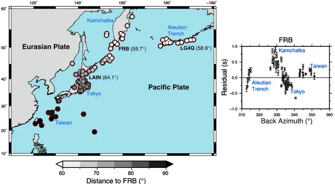
Figure 4. Earthquakes corresponding to the source side feature for station FRB plotted against back azimuth and on a map. Residual value is strongly correlated
with distance to FRB. Station labels on the map indicate approximate location and distance to the event at the peak of the source side feature for the three affected stations from Figure 3.
(difference between predicted and observed ray parameter). However, histograms comparing anomalies between affected and unaffected stations reveal that neither parameter was correlated with the source side effect (Figure 3b). We also examined the raypaths for the earthquakes for each of the affected stations to determine whether they followed any lithospheric terrane boundary or indicate the presence of any particu-lar structure. No such boundary or lateral interface was found at depths up to 300 km, however (see figure of piercing points in the supporting information). Body wave energy from teleseismic earthquakes arrives nearly vertically at the receiver, so any receiver-side structure that could produce such wildly varying residuals would have to be present beneath every red station in Figure 3a. We consider it a more likely and simpler explana-tion that the structure in quesexplana-tion affected the seismic waves close to their mutual source. The effect appears to be dependent upon source-receiver distance along subduction trench systems oriented approximately parallel to the earthquake-receiver GCP. Multipathing of the wavefront, which happens when the wavefront crosses itself due to complicated velocity structure, could also affect the recorded arrival times (Rawlinson & Sambridge, 2003). However, multipathing is expected to be incoherent between stations (Vandecar & Crosson, 1990), and the adaptive stacking procedure of section 4.2 does not work on incoherent arrivals. A more plausible explanation is that the subduction zone from which the affected earthquakes emerge acts as a waveguide to energy emitted along its strike. We analyzed the seismogram frequency content of affected and unaffected rays to further test our source side contamination hypothesis (Figure 3c). Affected seismo-grams display an enhancement of frequencies>1 Hz, and particularly between 2 and 3 Hz, when compared to unaffected rays. This frequency characteristic is independent of whether the relative arrival-time residuals are positive or negative (Figure 3d), so the source side structure can apparently cause P waves to speed up and slow down. Local studies of the subduction zone in Japan have suggested that the subducted oceanic mantle lithosphere can act as a high velocity, low attenuation, waveguide (e.g., Abers, 2005; van der Hilst & Snieder, 1996). Early arrivals are elegantly explained in this way, but some of the source side-affected arrivals we observe are relatively late and therefore require an alternative explanation. The thin (<10 km) layer of subducted oceanic crust beneath Japan is also known to act as a slow-velocity waveguide (e.g., Garth & Rietbrock, 2014) and can enhance high-frequency (2–3 Hz) body wave energy (e.g., Furumura & Kennett, 2008). We speculate, therefore, that the energy arriving at the red stations in Figure 3a has been affected to some degree by the subducted plate beneath Japan, whether it be its crust, mantle lithosphere, or both.
Figure 5. Station map showing network subsets and their respective results of restacking for two representative stations. Subsets are indicated by colored loops:
Green—Small Model; orange—West Model; pink—East Model. The Large Model group includes all stations in the network.
We tested the pervasiveness of the source side TRES feature with parallel data sets consisting of fewer stations: a Small Model eliminating the northern and southern most receivers, an East Model using only stations from Southampton Island and eastward, and a West Model using only stations from Southampton Island and westward (Figure 5). The effect was much more pronounced for the P waves than the S waves, so this analysis was restricted to the P wave data set. Note that all data were completely restacked in each subset. This is necessary because the regional mean may change every time a receiver is removed from the network. The results of restacking the smaller model space data show that the source side TRESfeature is effectively eliminated for the smaller models (side panels of Figure 5): the peak-to-peak spread for the two represen-tative stations has reduced from ±1 to ±0.5 s. The implication is that the source side effect does not cause significant variations in data over a smaller network area, and the TRES feature is therefore eliminated by removing the regional mean in equation (4). Network apertures>1,200 km may therefore be prone to source side structure contamination, at least from subduction zones oriented parallel to the GCP. We can contribute only one network-source region observation, so we cannot confidently constrain the degree of alignment between GCP and subduction zone strike at which contamination of the receiver-side residuals begins. Careful examination of the orientation of subduction zones from source regions relative to the network should be considered, and input data should always be examined closely before inversion. We revisit this issue, including how and whether it affects our inversions, in section 5.1.
4.4. Tomographic Inversion Procedure 4.4.1. FMTOMO
The inversion code used in this study is the Fast Marching TOMOgraphic (FMTOMO) method of Rawlinson et al. (2006) to solve for upper mantle seismic structure. Two grids of nodes are defined to make up the model space. The velocity grid is made of the unknowns in the inversion that control the velocity field, and the propagation grid is used to track the wave field through the model space during the forward step of the inversion. FMTOMO uses the Tau-P method (Kennett & Engdahl, 1991) to compute ray travel times from the source to the edge of the local 3-D model region and then applies a grid-based eikonal solver, known as the Fast Marching Method, to track wavefronts with a propagation grid to the surface through velocity structure which may vary radially
S5 D7 Roughness (1/kms) x 10^-5 0 2 6 8 Residual (ms) 200 210 220 230 240 250 260 270
280 P-wave Residual vs Roughness
4 Roughness (1/kms) x 10^-5 0 0.5 1 1.5 2 2.5 Residual (ms) 200 250 300 350 400 450 500 550 600 650 S5 D5
S-wave Residual vs Roughness
Figure 6. Trade-off areas for regularization parameters forSandPwave speed models. Each colored line represents a single damping value, each dot a different smoothing value. Values for both parameters were varied in the sequence: 0.1, 0.5, 1, 3, 5, 7, 10, 15, 30, 50, and 100. The approximate values of the central region are indicated by the green dots and dashed lines.
and laterally. This propagation grid is not used to define the model but simply represents a discrete sampling at some specified resolution. During inversion FMTOMO minimizes the objective function:
S(m) =1
2[Ψ(m) +𝜖Φ(m) + 𝜂Ω(m)] (5)
The value m refers to the model parameters that are changed during the inversion. The first term, Ψ(m), is minimized when the model travel times match as closely as possible the observed travel times. The second term Φ(m) penalizes models that differ from the reference or starting model m0. The third term, Ω(m),
penal-izes model roughness. The regularization terms,𝜂 and 𝜖, control damping (similarity to starting model) and smoothing (degree of model roughness), respectively. Ideally, we seek a model that satisfies the data but is also smooth and as close to the starting model as possible.
Through extensive testing of the model space we determined the regularization parameters via trade-off curve analysis that balanced data fit with model roughness. The residual value in Figure 6 is a measure of how much of the input data is unexplained by the model; a low residual means a higher data fit. A high data fit may require an unrealistically rough model, and an overly smooth model may miss important structure. Typically, the parameters that produce the knee of a trade-off curve between roughness and data misfit are understood to be the best choice. We produced inversions of the input data for every combination of a sequence of both smoothing and damping values of 0.1–100. When plotted together, these give a trade-off area rather than a single curve. The center point of the trade-off area is chosen for the final model inversions (Figure 6).
4.4.2. Crustal Modeling
Moho topography and crustal velocity structure can have a significant influence on teleseismic travel times (e.g., Waldhauser et al., 2002). To mitigate this problem, we applied a crustal velocity and Moho model devel-oped from receiver function and surface wave inversion results (Gilligan et al., 2016). Moho topography in northern Hudson Bay is significant; ∼7 km deeper beneath Baffin Island than the Archean regions to the west (e.g., Thompson et al., 2010). Moho depth estimates from Gilligan et al. (2016) at each station were interpolated to produce a continuous interface and inserted into the initial FMTOMO model space. Likewise, the modeled crustal velocity values were sampled every 2 km beneath each station and interpolated to create a layer with its base defined by the Moho model. Data fitting was best when the crustal models of Gilligan et al. (2016) were fixed in our inversions rather than allowed to vary.
4.4.3. Resolution Testing
To test the resolving ability of our data set, we performed synthetic checkerboard resolution tests. The pre-dicted arrival times for our earthquakes are calculated through a model space with ±0.4 km/s checkers (relative to ak135). We then use those predicted times as input data for an inversion. This test attempts to give a realistic visualization of where the data set can recover velocity anomalies, and what size of anomaly might be resolvable. Our network has variable station spacing, the shortest being 100–200 km in the Hudson Strait,
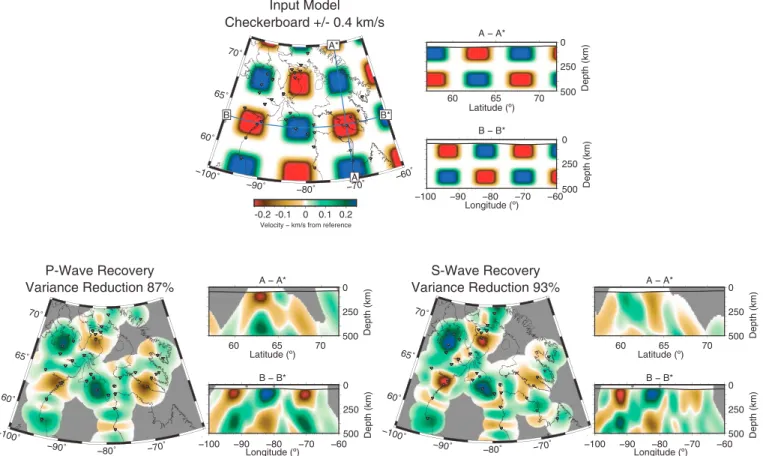
Figure 7. Checkerboard resolution tests forPandSwave model spaces. Cross-sections A-A* and B-B* shown in the input model are the same for bothPandS
wave recovery models. Slices at 180-km depth. Highest resolution is in the central region of the model, the eastern Churchill plate, and the Hudson Strait.
southern Baffin Island, and the eastern Rae domain. The input checkers in Figure 7 are ∼300 × 300 km hori-zontally and are 120-km thick but vary slightly with latitude. This length-scale governs the minimum size of feature that can be resolved by this model in regions of minimum station coverage.
The recovered inversion model in Figure 7 can be compared to the input checkerboard model to see where we have good resolution and the degree to which anomalies are smeared. The gray mask excludes regions of the model space where no raypaths travel. Model recovery is similar for P and S wave models, although the P recovery is everywhere better, with best resolution along the Hudson Strait and northern islands region (transect B-B*: Figure 7). Other regions, especially central Hudson Bay itself, have relatively poor resolution due to a lack of stations and the near-vertical incidence of teleseismic arrivals. Vertical smearing is low in the central portions of the model, and worst near the edges of the model space where fewer crossing rays can be expected. Vertical smearing like this is typical of body wave tomography studies because the energy from teleseismic earthquakes arrives nearly vertically beneath the receivers.
5. Results
5.1. Source Side Structure in Inversions
Before interpreting our results in terms of Hudson Bay upper mantle seismic structure, we must deter-mine how the source side structure problems identified in section 4.3 (Figures 3 and 4) affect our models. Specifically, we forward model travel times in the top 300 km and, separately, the bottom 300 km of our tomographic model, then compare synthetic and observed travel time residuals. This lets us test whether spurious structure is mapped into the upper portions of our model where we make structural interpreta-tions or whether it falls into the deeper, less-well-resolved and uninterpreted parts. The results are shown for three example stations, FRB, LG4Q, and LAIN (matching Figure 3) because their wide spacing illustrates the pervasiveness of the effect.
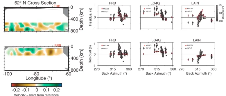
Figure 8. Forward modeling results for stations FRB, LG4Q, and LAIN at back azimuths of 270–360∘through either the top 300 km or bottom 300 km of the full inversion model. These match the stations shown in Figure 3. Tracing through the bottom 300-km model recreates the source side feature quite well, while tracing through the top 300-km model does not. This indicates that the feature in the back azimuth plots is entirely explained by the deepest structure in the model space, and the upper 300 km seems unaffected. The approximate location of station FRB is indicated by the red text.
Our full model space extends to 800-km depth. Residuals calculated with only the bottom 300 km of the inverted model region active accommodate much of the source side feature (Figure 8). The model with only the top 300 km of the model space active has no indication of the source side feature. This indicates that the inversion code is placing structure to explain the source side contaminated data in the less-constrained, deep-est 300 km of the model space. We can thus safely interpret structure in the upper 500 km of the full model. Parameterizing tomographic models deeper than the resolving power of the teleseismic data set is common (e.g., Vandecar et al., 1995; Villemaire et al., 2012). Our work demonstrates that this approach is particularly important for large aperture (>1,000 km) networks.
5.2. P and S Wave Inversion Models
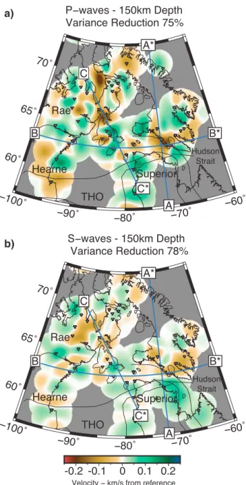
The P and S wave tomographic models in Figures 9 and 10 show significant heterogeneous mantle wave speed structure in northern Hudson Bay and Nunavut. The depth slices are presented at a midlithospheric depth of 150 km, and depth variation is shown via the cross sections. The Quebec-Baffin transect (cross-section A-A*) reveals slow wave speed structure extending to at least 500 km in the Hudson Strait, with faster wave speeds in the Superior craton to the south and the Churchill to the north for both P and S waves. A laterally robust slow wave speed curtain extending east-west through the northern portion of Hudson Bay (cross-section B-B*), then turning northward toward the east coast of southern Baffin Island, is also imaged in both models. The western portion of the B-B* cross section is fast in the P wave model but appears slow in the S wave model. Just northward, within our station coverage, both P and S wave models in Figure 9 image a low wave speed anomaly on Southampton Island in the center of the model space. The S wave model (Figure 9b) sees this anomaly extend southward where it intersects with the B-B* transect, while the P wave model does not (Figure 9a). This discrepancy is less likely due to actual structural variations and more likely a result of the model being underconstrained due to a lack of stations in the central part of Hudson Bay. A sharp, vertical change in seismic wave speed occurs beneath Southampton Island (cross-section C-C*) in the P wave model, with a similar, although less-pronounced, feature in the S wave model. This is as strong an anomaly as the THO-related feature to the east.
Our inversion model has resolution in the Archean central Rae and Hearne cratons (Figure 7), and results indicate a complex and heterogeneous velocity pattern within the shield region. There exists a low-velocity anomaly (north end of C-C* in Figure 9) near the connection of Melville Peninsula to the main Rae landmass (Figure 1), and its shape differs between the P and S wave models more substantially than anomalies to the east beneath Hudson Bay and Baffin Island.
-0.2 -0.1
0
0.1 0.2
A
A*
B
B*
C
C*
THO
a)
b)
A
A*
B
B*
C
THO
C*
Figure 9. ThePandSwave inversion depth slices at 150-km depth. Both models reveal broadly similar structure. Variance reduction 75% from 0.11 s2forPwaves and 78% from 0.8 s2forSwaves.
The inversion models discussed in this section were created using the entire data set. P wave inversion models for each of the subsets, Small Model, East Model, and West Model, are included in the supporting information. Each subset’s inversion model differs slightly from the larger model due to the lower resolving power of the smaller network, but they all share the same first-order characteristics where they overlap spatially. This provides support for the robustness of the anomalies shown in Figures 9 and 10.
6. Discussion
6.1. Causes of Seismic Heterogeneity and Comparison to Previous Tomographic Studies
As explained in section 3, global models of Hudson Bay seismic structure have imaged uniformly fast wave speeds in the upper ∼250 km of the mantle. Our relative arrival-time inversion approach constrains het-erogeneities with respect to a regional, not global, mean, however. For example, the mean S wave velocity anomaly at permanent station FRB in the global model of Ritsema et al. (2011) is 𝛿VS ≈ 2.5%. However,
Superior THO Churchill
Hearne THO Baffin Island
Hudson Plutons Superior Sugluk? THO Rae
S-wave Model
P-wave Model
-0.2 -0.1
0
0.1 0.2
THO 60 70 Latitude (°) 65 S N THO -100 -90 -70 -60 °) -80 W E 0 500 1000 1500 W E THO 60 70 Latitude (°) 65 S N500
300
100
THO -100 -90 -70 -60 °) -80 W E500
300
100
0 500 1000 1500 W E500
300
100
Figure 10. Lithospheric cross-sections for bothPandSwave inversions along profiles defined in Figure 9. Labels and colors of geological units correspond to Figure 1.
the mean relative arrival time residual for FRB in our study is near zero (0.2 s), meaning both high and low-velocity anomalies in our models (Figures 9 and 10) are likely fast compared to the global mean and thus reflect wave speed heterogeneity within the Canadian Shield (Bastow, 2012).
Surface erosion of cratonic regions like northern Hudson Bay results in loss of radiogenic particles and there-fore an anomalously low heat flow (≤50 mW/m2, e.g., Levy et al., 2010). Fast wave speed cratonic roots or keels are thus often considered>200∘C cooler than surrounding, younger terranes (e.g., Mareschal et al., 2004). Ele-vated mantle temperatures and associated partial melt can cause low seismic wave speeds (e.g., Allen et al., 2002; Bastow et al., 2008) but are inappropriate hypotheses for seismic heterogeneity in our study area since it is thought to be cooler than average at upper mantle depths (Goes & van der Lee, 2002). Anisotropy may also influence wave speed variations in northern Hudson Bay (e.g., Darbyshire et al., 2013; Liddell et al., 2017). How-ever, the general consistency between our P wave and S wave models (Figures 9 and 10) despite approximately perpendicular particle motion between the phases, and our good back azimuthal coverage of earthquakes (Figure 1), implies that this is not a predominant factor, and that our models are dominated by isotropic wave speed variations. Our tomographic images, with their higher lateral resolving power than earlier
surface wave studies, illuminate the finer-scale internal architecture of the northern Hudson Bay region. Other relative arrival time studies of nearby regions (e.g., Boyce et al., 2016; Frederiksen et al., 2013) included terranes or geological features that ranged in age from Archean to Phanerozoic. The peak-to-peak residual amplitudes of studies like these are to some degree set by the age range of the structures within the model space. Our study, in contrast, spans only Precambrian lithosphere, and thus, our models tend to highlight internal variations in Precambrian lithospheric structure rather than the typically more pronounced contrasts between Precambrian and Phanerozoic lithosphere.
The eastern edge of southern Baffin Island in our models exhibits a low-velocity anomaly for both P and S waves at lithospheric depths. S wave perturbations at 150-km depth in the continent-scale model of Schaeffer and Lebedev (2014) show a sharp boundary to the cratonic lithosphere in this region, following closely the eastern coast of Baffin Island. Lithospheric thinning in this area has occurred since the opening of Baffin Bay separating Canada from Greenland in the late Jurassic to early Cretaceous (Larsen et al., 1999; Oakey & Chalmers, 2012). Our models are therefore imaging the edge of low-velocity material associated with the asthenosphere at the Churchill craton’s edge.
6.2. Mantle Seismic Structure of the Churchill Plate
With acceptable resolution for much of the central Rae and northern Hearne domains (Figure 7), we image considerable seismic heterogeneity throughout the Churchill plate. Our study may be expected to image seismic variation that has not previously been resolved by global studies because of our greater number of stations and better data coverage. Surface wave studies also have naturally low lateral resolution compared to teleseismic body wave tomography.
Marked seismic heterogeneity within Precambrian domains has been observed worldwide (e.g., Australia, Fishwick & Rawlinson, 2012; China, Tian et al., 2009; Fennoscandia, Bannister et al., 1991). Internal cratonic velocity variations of the southern African Kaapvaal craton were observed to be very small (∼0.5%); however, low-velocity anomalies were modeled within the eastern edge of the Kaapvaal craton (Fouch et al., 2004; Youssof et al., 2015). Called the Bushveld Complex, this anomaly has been associated with ∼2.0-Ga Proterozoic chemical modification and mantle refertilization (James et al., 2001; Youssof et al., 2015). Similar examples of cratonic collisions initiating metasomatism and creating fertile, low-velocity mantle regions include Siberia (Griffin et al., 2005), and the central Superior province (Boyce et al., 2016).
The seismic velocity variations in our region are not easily explained by age: the boundary between the Paleoarchean Rae and the Mesoarchean Hearne cratons (STZ) is not correlated with a consistent change in wave speed at lithospheric depths (Figure 11). While a number of faults and gravity gradients have been defined in the central Rae craton (e.g., Snyder et al., 2015), we do not observe mantle expression or corre-lation to any of these delineations within either the P or S wave models (Figures 9 and 10). Diamondiferous kimberlites are expected to correlate with thick lithosphere and therefore fast velocity anomalies; however, our models show no obvious correlation with diamond prospects (Figure 1). Magnetotelluric studies within the western Hearne in Alberta and in the Yellowknife Fault Zone in the Yukon, also attributed upper mantle conductive anomalies to widespread metasomatism (Jones & Garcia, 2002; Nieuwenhuis et al., 2014). The Hudson Plutons are 1.85- to 1.81-Ga intrusive granites interpreted as post-orogenic lower crustal intru-sions hosting crustal melt or metasomatic materials found throughout the Churchill domain but concentrated near the west coast of northern Hudson Bay near Melville Peninsula (Figure1; Berman et al., 2005; Peterson et al., 2012). They are associated with a Bouguer gravity anomaly low and near-vertical conductive anomalies imaged with magnetotellurics interpreted to be carbon films or leftover water (Spratt et al., 2014). These inver-sions also showed that upper mantle resistivity changed significantly between various lithospheric blocks, increasing from Baffin Island south to the STZ. Consistent with earlier geological work (e.g., Hynes & Rivers, 2010), Boyce et al. (2016) interpreted slower-than-expected wave speeds beneath the Grenville Front as evidence for metasomatic modification of the Superior lithosphere during the 250-Ma subduction process. The resulting wave speed anomalies are of the order of ±1.5%, significantly smaller than those we observe (∼4% below Melville peninsula). As far as we have can determine, no petrological studies have claimed large-scale metasomatic modification of the Melville lithosphere. Therefore, since THO tectonism acted for a much shorter period (∼80 Ma) than during the Grenville orogen, we consider metasomatism only par-tially capable of explaining our velocity anomalies. The remainder of the anomalous structure likely reflects inherent compositional differences between lithospheric blocks, unrelated to metasomatic modification. We interpret our Rae anomaly (Figures 9 and 10) to reflect a combination of metasomatism and compositional
Rae
Hearne
STZRae
Hearne
STZDistance (km)
P-Waves
STZS-Waves
Depth (km)
Distance (km)
STZS
N
S
N
2
Figure 11. ThePandSwave inversion models with cross sections across the Snowbird Tectonic Zone (STZ). Neither model images a velocity distinction across the interface.
differences between constituent lithospheric blocks; the metasomatism being driven by the same forces that created the crustal melts of the Hudson Plutons.
6.3. Mantle Seismic Structure of the Trans-Hudson Orogen and Implications for Precambrian Plate Tectonics
A striking feature in Figures 9 and 10 is the strong slow wave speed feature that curves around the Quebec mainland and through the Hudson Strait and then angles northeast beneath the Archean crust of southern Baffin Island (B-B*). Gilligan et al. (2016) found compelling similarities between the crustal velocities of the Tibetan Plateau and southern Baffin Island, allowing for ∼30 km of erosion since completion of the THO. Recent modeling of seismic anisotropy using back azimuthal variation of shear wave splitting parameters in southern Baffin Island strongly suggested the presence of dipping anisotropy and related that to subducted material from the THO (Liddell et al., 2017). These geophysical studies support a growing number of geo-logical studies that consider the THO reminiscent of a modern-style subduction zone (e.g., St-Onge et al., 2009; Weller & St-Onge, 2017). Our tomographic inversions clearly image low-velocity material from the THO that extends beneath the Archean terranes of southern Baffin Island (A-A* in Figures 9 and 10). We interpret this anomaly as being due to compositionally distinct Proterozoic material underthrust beneath the Archean Churchill craton during the THO in a modern-style tectonic collision.
A further strong velocity contrast manifests near Southampton Island in both P and S wave models (Figures 9 and 10). Higher velocities in the east give way to lower velocities to the northwest into the Rae domain. Con-sidering the interpretation of plate tectonic activity, this contrast is most likely due to a lithospheric boundary from an Archean microcontinent, caught in between the Churchill and the Superior during the THO. Inter-pretations of a terrane boundary in this region were also made from SKS splitting (Liddell et al., 2017) and magnetotelluric data (Spratt et al., 2012); however, Gilligan et al. (2016) found no clear difference in crustal structure between the various northern Hudson Bay islands. This indicates either alteration of the mantle or underthrusting of mantle material from a nearby terrane beneath Southampton Island. A possible candidate
for this is the Sugluk block, a Mesoarchean terrane of high grade metamorphic rocks considered distinct from its surrounding blocks due to a lack of 2.5- to 2.6-Ga magmatism (e.g., Corrigan et al., 2009; Hoffman, 1985). The Sugluk is exposed on the northwestern tip of Quebec where it is intruded by plutonic rocks of the Narsajuaq arc (e.g., Dunphy & Ludden, 1998; St-Onge et al., 2002). Bouguer gravity and aeromagnetic signatures indi-cate that it extends north to Baffin Island and west beneath Hudson Bay into the region where we observe the velocity interface (Corrigan et al., 2009).
The Snowbird Orogeny took place during the initiation of the THO and ended<0.1 Ga before terminal collision of the Superior and Churchill (Berman et al., 2007; Corrigan et al., 2009). The result was the>2,800-km-long suture zone between the Rae and the Hearne domains. Cross sections of the P and S wave model in Figure 11 show no consistent mantle velocity distinction between the domains divided by the STZ. Neither have studies of lithospheric anisotropy found evidence for fabrics that parallel any potential tectonic boundary at the STZ (e.g., Liddell et al., 2017; Snyder et al., 2013). However, the lack of stations south of the STZ means we cannot provide a more detailed discussion of its structure. Our results are most consistent with an interpretation of the STZ as a relatively minor event involving what might be considered a tributary of the much larger Manikewan ocean whose closure initiated the THO (Corrigan et al., 2009). This process brought together two blocks that were of relatively similar composition from a seismic wave speed perspective, and on too small a scale to create the features we image for the THO to the east.
7. Conclusions
We have presented new P and S wave tomographic inversions for the northern Hudson Bay region of Canada using a combined network of temporary and permanent broadband seismograph stations. Our results constitute the most comprehensive body wave tomographic model of northern Hudson Bay to date. We have shown that sources with raypaths approximately parallel to subduction zones may include some source side influence after relative arrival processes and removal of the mean. We further show that this effect can be mitigated to some degree by limiting network size and carefully examining where spurious structure may be mapped into the inversion. Nevertheless, our work shows that source-network orientations and back azimuth residual patterns should be closely examined to ensure that the results truly represent only local structure.
The Archean Rae and Hearne domains exhibit complex internal structure, implying a complex accretionary history. However, there is no seismic velocity evidence for a terrane boundary across the Snowbird Tectonic Zone (Rae-Hearne suture), consistent with the view that it was a relatively short-lived orogeny of modest scale. A strong velocity contrast at shallow depths on and around Southampton Island in northern Hudson Bay is interpreted as a microcontinent (Sugluk block) with a collisional history distinct from the Churchill plate to the north and the Superior plate to the south.
We interpret slow wave speeds between the Superior and Churchill plates as Paleoproterozoic THO material caught between the Archean colliders as part of a modern-style plate tectonic event. Low-velocity anomalies persist beneath the Churchill province, but not beneath the Archean Superior province. We interpret this as strong evidence for 1.8-Ga Paleoproterozoic plate-scale underthrusting.
References
Abers, G. A. (2005). Seismic low-velocity layer at the top of subducting slabs: Observations, predictions, and systematics. Physics of the Earth
and Planetary Interiors, 149, 7–29.
Abt, D. L., Fischer, K. M., French, S. W., Ford, H. A., Yuan, H., & Romanowicz, B. (2010). North American lithospheric discontinuity structure imaged by Ps and Sp receiver functions. Journal of Geophysical Research, 115, B09301. https://doi.org/10.1029/2009JB006914 Allen, R. M., Nolet, G., Morgan, W. J., Vogfjörd, K., Bergsson, B. H., Erlendsson, P., et al. (2002). Imaging the mantle beneath Iceland using
integrated seismological techniques. Journal of Geophysical Research, 107(B12), 2325. https://doi.org/10.1029/2001JB000595 Bannister, S. C., Ruud, B. O., & Husebye, E. S. (1991). Tomographic estimates of sub-Moho seismic velocities in Fennoscandia and structural
implications. Tectonophysics, 189(1-4), 37–53.
Bao, X., & Eaton, D. W. (2015). Large variations in lithospheric thickness of western Laurentia: Tectonic inheritance or collisional reworking?
Precambrian Research, 266, 579–586.
Bastow, I. D. (2012). Relative arrival-time upper-mantle tomography and the elusive background mean. Geophysical Journal International,
190(2), 1271–1278.
Bastow, I. D., Eaton, D. W., Kendall, J.-M., Helffrich, G., Snyder, D. B., Thompson, D. A., et al. (2015). The Hudson Bay Lithospheric Experiment (HuBLE): Insights into Precambrian plate tectonics and the development of mantle keels. Geological Society, London Special Publications,
389, 41–67.
Acknowledgments
The authors would like to thank A. Boyce, L. Petrescu, and C. Ogden of the ICcratons group as well as S. Goes for numerous enlightening conversations about Canadian Precambrian geology and beyond. In addition, the authors thank both reviewers, as well as the Editor, Savage, for their thoughtful comments and improvements. M. V. Liddell is funded by an Imperial College President’s Scholarship. F. A. Darbyshire is supported by the Natural Sciences and Engineering Research Council of Canada. The data used in this study are available for download via POLARIS or the IRIS DMC, and the processed relative arrival time data set and the 3-D tomographic models are available for download as a digital supplement. Further questions can be directed to M. V. Liddell ([email protected]).
Bastow, I. D., Kendall, J. M., Helffrich, G. R., Thompson, D. A., Wookey, J., Brisbourne, A. M., et al. (2011). The Hudson Bay lithospheric experiment. Astronomy and Geophysics, 52(6), 21–24.
Bastow, I. D., Nyblade, A. A., Stuart, G. W., Rooney, T. O., & Benoit, M. H. (2008). Upper mantle seismic structure beneath the Ethiopian hot spot: Rifting at the edge of the African low-velocity anomaly. Geochemistry, Geophysics, Geosystems, 9, Q12022. https://doi.org/10.1029/2008GC002107
Berman, R. G., Davis, W. J., & Pehrsson, S. (2007). Collisional Snowbird tectonic zone resurrected: Growth of Laurentia during the 1.9 Ga accretionary phase of the Hudsonian orogeny. Geology, 35(10), 911–914.
Berman, R. G., Sanborn-Barrie, M., Rayner, N., & Whalen, J. (2013). The tectonometamorphic evolution of Southampton Island, Nunavut: Insight from petrologic modeling and in situ SHRIMP geochronology of multiple episodes of monazite growth. Precambrian Research,
232, 140–166.
Berman, R. G., Sanborn-Barrie, M., Stern, R. A., & Carson, C. J. (2005). Tectonometamorphism at ca. 2.35 and 1.85 Ga in the Rae domain, western Churchill Province, Nunavut, Canada: Insights from structural, metamorphic and in situ geochronological analysis of the southwestern Committee Bay belt. The Canadian Mineralogist, 43(1), 409–442.
Boyce, A., Bastow, I. D., Darbyshire, F. A., Ellwood, A. G., Gilligan, A., & Menke, W. (2016). Subduction beneath Laurentia modified the North American craton edge: Evidence fromPandS-wave tomography. Journal of Geophysical Research: Solid Earth, 121, 5013–5030. https://doi.org/10.1002/2016JB012838
Corrigan, D., Pehrsson, S., Wodicka, N., & de Kemp, E. (2009). The Palaeoproterozoic Trans-Hudson Orogen: A prototype of modern accretionary processes. Geological Society, London, Special Publications, 327(1), 457–479.
Darbyshire, F. A., & Eaton, D. W. (2010). The lithospheric root beneath Hudson Bay, Canada from Rayleigh wave dispersion: No clear seismological distinction between Archean and Proterozoic mantle. Lithos, 120(1-2), 144–159.
Darbyshire, F. A., Eaton, D. W., & Bastow, I. D. (2013). Seismic imaging of the lithosphere beneath Hudson Bay: Episodic growth of the Laurentian mantle keel. Earth and Planetary Science Letters, 373, 179–193.
Davis, W. J., Hanmer, S., Tella, S., Sandeman, H. A., & Ryan, J. J. (2006). U-Pb geochronology of the MacQuoid supracrustal belt and Cross Bay plutonic complex: Key components of the northwestern Hearne subdomain, western Churchill Province, Nunavut, Canada. Precambrian
Research, 145(1-2), 53–80.
Dunphy, J. M., & Ludden, J. N. (1998). Petrological and geochemical characteristics of a Paleoproterozoic magmatic arc (Narsajuaq terrane, Ungava Orogen, Canada) and comparisons to Superior Province granitoids. Precambrian Research, 91(1-2), 109–142.
Eaton, D. W., Adams, J., Asudeh, I., Atkinson, G. M., Bostock, M. G., Cassidy, J. F., et al. (2005). Investigating Canada’s lithosphere and earthquake hazards with portable arrays. Eos, Transactions American Geophysical Union, 86(17), 169.
Fishwick, S., & Rawlinson, N. (2012). 3-D structure of the Australian lithosphere from evolving seismic datasets. Australian Journal of Earth
Sciences, 59(6), 809–826.
Fouch, M. J., James, D. E., VanDecar, J. C., & van der Lee, S. (2004). Mantle seismic structure beneath the Kaapvaal and Zimbabwe Cratons.
South African Journal of Geology, 107(1-2), 33–44.
Frederiksen, A. W., Bollmann, T., Darbyshire, F., & van der Lee, S. (2013). Modification of continental lithosphere by tectonic processes: A tomographic image of central North America. Journal of Geophysical Research: Solid Earth, 118, 1051–1066. https://doi.org/10.1002/jgrb.50060
Frederiksen, A. W., Miong, S. K., Darbyshire, F. A., Eaton, D. W., Rondenay, S., & Sol, S. (2007). Lithospheric variations across the Superior Province, Ontario, Canada: Evidence from tomography and shear wave splitting. Journal of Geophysical Research, 112, B07318. https://doi.org/10.1029/2006JB004861
Furumura, T., & Kennett, B. (2008). A scattering waveguide in the heterogeneous subducting plate. Advances in Geophysics, 7(50), 195–217. Garth, T., & Rietbrock, A. (2014). Downdip velocity changes in subducted oceanic crust beneath Northern Japan—Insights from guided
waves. Geophysical Journal International, 198(3), 1342–1358.
Gibb, R. A. (1983). Model for suturing of Superior and Churchill plates: An example of double indentation tectonics. Geology, 11(7), 413–417. Gilligan, A., Bastow, I. D., & Darbyshire, F. A. (2016). Seismological structure of the 1.8 Ga Trans-Hudson Orogen of North America.
Geochemistry, Geophysics, Geosystems, 17, 2421–2433. https://doi.org/10.1002/2016GC006419
Goes, S., & van der Lee, S. (2002). Thermal structure of the North American uppermost mantle inferred from seismic tomography.
Journal of Geophysical Research, 107(B3), 2050. https://doi.org/10.1029/2000JB000049
Griffin, W. L., Natapov, L. M., O’Reilly, S. Y., van Achterbergh, E., Cherenkova, A. F., & Cherenkov, V. G. (2005). The Kharamai kimberlite field, Siberia: Modification of the lithospheric mantle by the Siberian Trap event. Lithos, 81(1-4), 167–187.
Hawkesworth, C. J., Cawood, P. A., Dhuime, B., & Kemp, T. I. S. (2017). Earth’s continental lithosphere through time. Annual Review of Earth
and Planetary Sciences, 45, 169–198.
Hoffman, P. F. (1985). Is the Cape Smith Belt (northern Quebec) a klippe? Canadian Journal of Earth Sciences, 22, 1361–1369.
Hoffman, P. F. (1988). United Plates of America, the birth of a craton: Early Proterozoic assembly and growth of of Laurentia. Annual Review
of Earth and Planetary Sciences, 16, 543–603.
Hopkins, M., Harrison, T. M., & Manning, C. E. (2008). Low heat flow inferred from>4 Gyr zircons suggests Hadean plate boundary interactions. Nature, 456(7221), 493–496.
Hynes, A., & Rivers, T. (2010). Protracted continental collision—Evidence from the Grenville Orogen. Canadian Journal of Earth Sciences, 47, 591–620.
James, D. E., Fouch, M. J., VanDecar, J. C., van der Lee, S., & the Kaapvaal Seismic Group (2001). Tectospheric structure beneath southern Africa. Geophysical Research Letters, 28(13), 2485–2488.
Jones, A. G., & Garcia, X. (2002). Electrical resistivity structure of the Yellowknife River Fault Zone and surrounding region. In Gold in the
Yellowknife Greenstone Belt, North-west Territories: Results of the EXTECH III multidisciplinary research project, Special Publication No. 3. St. John’s (Chap. 10, pp. 126–141). Newfoundland, Canada: Geological Association of Canada, Mineral Deposits Division.
Kennett, B. L. N., & Engdahl, E. R. (1991). Traveltimes from global earthquake location and phase identification. Geophysical Journal
International, 105(2), 429–465.
Kennett, B. L. N., Engdahl, E. R., & Buland, R. M. (1995). Constraints on seismic velocities in the Earth from traveltimes. Geophysical Journal
International, 122(1), 108–124.
Larsen, L. M., Rex, D. C., Watt, W. S., & Guise, G. G. (1999).40Ar-39Ar dating of alkali basaltic dykes along the south-west coast of Greenland: Cretaceous and Tertiary igneous activity along the eastern margin of the Labrador Sea. Geology of Greenland Survey Bulletin, 184, 19–29. Lebedev, S., & van der Hilst, R. D. (2008). Global upper-mantle tomography with the automated multimode inversion of surface and S-wave
forms. Geophysical Journal International, 173(2), 505–518.
Levy, F., Jaupart, C., Mareschal, J. C., Bienfait, G., & Limare, A. (2010). Low heat flux and large variations of lithospheric thickness in the Canadian Shield. Journal of Geophysical Research, 115, B06404. https://doi.org/10.1029/2009JB006470