Statistical modeling of the ultra wide band propagation channel through the analysis of experimental measurements

HAL Id: hal-01912163

https://hal.archives-ouvertes.fr/hal-01912163

Submitted on 5 Nov 2018

HAL is a multi-disciplinary open access

archive for the deposit and dissemination of

sci-entific research documents, whether they are

pub-lished or not. The documents may come from

teaching and research institutions in France or

abroad, or from public or private research centers.

L’archive ouverte pluridisciplinaire HAL, est

destinée au dépôt et à la diffusion de documents

scientifiques de niveau recherche, publiés ou non,

émanant des établissements d’enseignement et de

recherche français ou étrangers, des laboratoires

publics ou privés.

Statistical modeling of the ultra wide band propagation

channel through the analysis of experimental

measurements

Pascal Pagani, Patrice Pajusco

To cite this version:

Pascal Pagani, Patrice Pajusco. Statistical modeling of the ultra wide band propagation channel

through the analysis of experimental measurements. Comptes Rendus Physique, Centre Mersenne,

2006, 7 (7), pp.762 - 773. �10.1016/j.crhy.2006.07.008�. �hal-01912163�

Physics

Statistical Modeling of the Ultra Wide Band Propagation Channel

through the Analysis of Experimental Measurements

Pascal Pagani

, Patrice Pajusco

a_{France Telecom Division Recherche et Développement, 4 rue du Clos Courtel, 35512 Cesson- Sévigné} b_{France Telecom Division Recherche et Développement, 6 avenue des Usines, 90000 Belfort}

Abstract

For the development of future Ultra Wide Band (UWB) communication systems, realistic modeling of the propagation channel is necessary. This paper presents an experimental study of the UWB radio channel, based on an extensive sounding campaign covering the indoor office environment. We consider the main characteristics of the UWB channel by studying the propagation loss and wide band parameters, such as the delay spread and the power delay profile decay. From this analysis, we propose a statistical channel model reproducing the UWB channel effects over the frequency bandwidth 3.1 GHz - 10.6 GHz. To cite this article: P. Pagani, P. Pajusco, C. R. Physique N (2006).

Résumé

Modélisation statistique du canal de propagation Ultra Large Bande par l’analyse de mesures expérimentales. Afin de développer les futurs systèmes de communication Ultra Large Bande (ULB), une modélisation réaliste du canal de propagation est nécessaire. Cet article présente une étude expérimentale du canal radio ULB, basée sur une campagne de sondage complète réalisée en environnement intérieur de bureau. Nous présentons les caractéristiques principales du canal ULB en termes de pertes par propagation, puis de paramètres large bande, comme la dispersion des retards et la pente du profil puissance-retard. À partir de ces analyses, nous proposons un modèle de canal statistique qui permet de reproduire les effets du canal ULB sur la bande de fréquences 3,1 GHz - 10,6 GHz. Pour citer cet article : P. Pagani, P. Pajusco, C. R. Physique N (2006).

Key words:Ultra Wide Band ; Radioelectric propagation ; Channel sounding ; Characterization ; Modeling Mots-clés :Ultra Large Bande ; Propagation radioélectrique ; Sondage de canal ; Caractérisation ; Modélisation

1. Introduction

Ultra Wide Band (UWB) is a radio communication technique using signals over an extremely wide frequency bandwidth, typically in the order of 500 MHz to several GHz. This particularity may be exploited to develop communication systems with data rates in the order of 500 Mbps for short range, indoor applications [1]. In 2002, the American regulation authority FCC allowed the emission of UWB signals in the 3.1 GHz - 10.6 GHz band [2]. Since then, the development of UWB communication systems has become an intensive research activity in both academic and industrial communities. In order to simulate and optimize such systems under realistic conditions, a thorough knowledge of the transmission channel properties is necessary. A considerable amount of work was already performed in this field, and a number of experimental sounding campaigns were set up in order to characterize the UWB propagation channel [3]. For instance, the IEEE 802.15.3a and IEEE 802.15.4a Task Groups developed UWB channel models for the simulation of system proposed for standardization [4, 5].

However, one may note that most of the analyses of the UWB propagation channel are based on sounding campaigns covering a reduced part of the FCC-defined frequency band. A few experimentations only were dimensioned to sound the entire 3.1 GHz - 10.6 GHz frequency band. [6–11]. This paper presents a characterization and modeling study of the UWB propagation channel, based on an extensive sounding campaign performed in the office indoor environment. A frequency domain sounding

Email addresses: pascal.pagani@francetelecom.com(Pascal Pagani), patrice.pajusco@francetelecom.com (Patrice Pajusco).

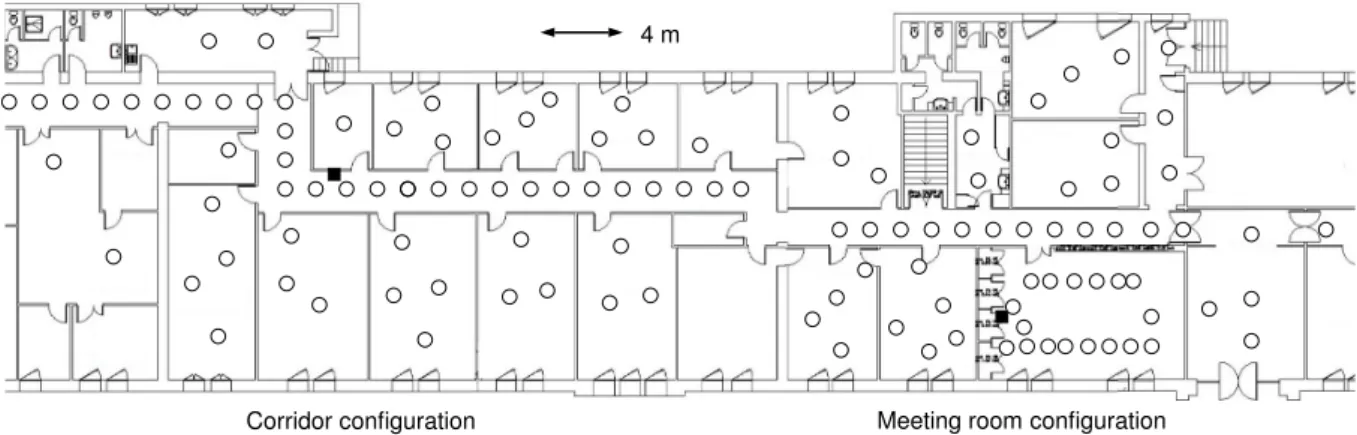
4 m

Corridor configuration Meeting room configuration

Figure 1. Measurement locations for the UWB sounding campaign. Black squares represent Rx locations, and white circles correspond to Tx locations.

technique was used, allowing for measurements over the 3.1 GHz - 11.1 GHz band. The statistical analysis of the measured data permitted to study the main characteristics of the UWB radio channel. From these experimental results, we propose a statistical model allowing fof the simulation of the ULB Channel Impulse Response (CIR) over any partial frequency band included within the 3.1 GHz - 10.6 GHz band.

We first present the sounding campaign and the issues linked to the antennas and the calibration procedure (Section 2). The different analyses performed to characterize the main UWB radio parameters are developed in Section 3. In particular, the propagation losses and the Power Delay Profile (PDP) structure are studied. Finally, Section 4 describes a statistical channel model which may be used for the realistic simulation of future UWB systems.

2. UWB Channel Sounding Campaign 2.1. Experimental Setup

In order to characterize the UWB propagation channel, a measurement campaign was performed in a typical indoor office environment, as presented on Fig. 1 [12]. A Vector Network Analyzer (VNA) was used to sound the radio channel over the

3.1 GHz - 11.1 GHz frequency band, following a classical S21parameter measurement procedure. A total of 4005 frequency

tones were sounded, which corresponds to a maximum delay of about 500 ns for the measured CIRs. At the emitter (Tx) and at the receiver (Rx), monoconical antennas CMA 118 were used. The Rx antenna was placed at a height of about 2.3 m in two different locations : in a meeting room and in a corridor. The Tx antenna was fixed at a height of 1.40 m on a rotating arm, allowing for the measurement of 90 CIRs around a circle of 40 cm in diameter. The rotating arm was placed at more than 120 locations, covering both Line-of-Sight (LOS) and Non Line-of-Sight (NLOS) locations configurations. We collected more than 10 000 CIRs, which served as a basis for the statistical analysis of the UWB radio channel. Depending on the Tx-Rx distance, up to three amplifiers were inserted in the measurement chain.

2.2. Antenna Effect and Calibration

All collected measurements were calibrated using a reference measurement, where the VNA input and output ports were directly connected using cables. When considering UWB channel sounding, a specific attention must be given to the effect of antennas on the measured data. The measurement antennas presented an omnidirectional radiation pattern in azimuth, but we observed significant variations of the antenna gain with the elevation. In addition, the global shape of the radiation pattern considerably varies when the frequency of operation increases from 3.1 GHz to 11.1 GHz. Hence, the antennas need to be precisely characterized and experimental data must be corrected accordingly. In our analysis, the 3D antenna radiation pattern was measured between 3 GHz and 10 GHz with a 1 GHz step. The measured Channel Transfer Function (CTF) was then adjusted with respect to the antenna gain in the Tx-Rx direction. More details regarding this calibration procedure are available in [12].

3. Experimental Characterization 3.1. Propagation Loss

A first analysis consisted in evaluating the propagation loss. The channel power attenuation, observed over the whole 3.1 GHz - 10.6 GHz band, is represented as a function of the Tx-Rx distance d for the global set of measurement points in Fig. 2. The

0.6 0.8 1 2 3 4 5 6 8 10 20 30 110 100 90 80 70 60 50 40 Distance (m) A tt e n u a ti o n ( d B ) LOS NLOS

Figure 2. Path loss as a function of distance. Each plot represents the median attenuation in the FCC band.

Sounding N σS(dB)

campaign LOS NLOS LOS NLOS

France Telecom 1.62 3.22 1.7 5.7 Kunisch et al. [6] 1.58 1.96 Alvarez et al. [8] 1.4 3.2 to 4.1 Buehrer et al. [7] 1.3 2.3 to 2.4 2.8 to 3.6 2.8 to 5.4 Cassioli et al. [9] 1.92 3.66 1.42 2.18 ITU [13] 1.7 3.5 to 7 1.5 2.7 to 4 Table 1

Comparison of the propagation loss parameters for different analyses of the UWB channel.

path loss in dB P L was then compared to the following theoretical formula using a least squares fitting procedure :

P L(d) = P L(d0) + 10N log

„ d

d0

«

+ S(d) (1)

where N represents the path loss exponent and d0is an a arbitrary distance of 1 m. The parameter S accounts for the channel

large scale fading and is characterized by its zero mean and its standard deviation σS.

In the LOS configuration, the observed value of the parameter N was 1.62, with a standard deviation σSof 1.7 dB. In the

NLOS configuration, the measurement plots are somewath more dispersed, with a parameter N = 3,22 and a standard deviation

σS = 5,5 dB. The value of the parameter P L(d0) was respectively assessed at 53.7 dB and 59.4 dB. Table 1 compares our

results with other published analyses performed over measurements covering the entire FCC-defined frequency band. For the sake of comparison, the values recommended by the standardization institute ITU have also been reported [13].

Finally, we studied the channel attenuation over different partial frequency bands of 528 MHz each. We concluded that

the main effect of the central frequency was an additionnal attenuation of 20 log“_ff

0

”

in Eq. (1), where f is the operating

frequency and f0is a reference frequency. More details about these results may be found in [12].

3.2. Delay Spread

From each set of M = 90 CIRs hm(τ ) measured locally, a Power Delay Profile (PDP) P (τ ) was computed as follows :

P (τ ) = 1 M M X m=1 |hm(τ )|2 (2)

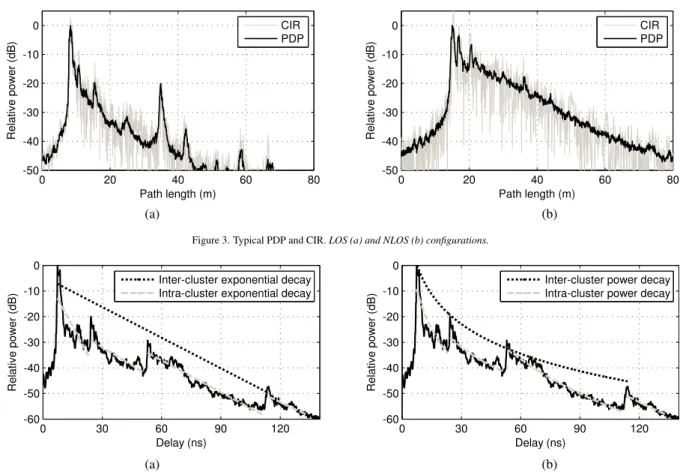
Figure 3 presents typical PDPs measured in LOS and NLOS configurations, along with one of the 90 constituting CIRs. Note that the delay on the x-axis has been converted in path length in meters for an easier interpretation of the propagation paths. In both LOS and NLOS situations, one may clearly observe one or several multipath clusters, corresponding to one main path followed by an exponentially decreasing diffuse power.

The delay spread τRM Swas computed for each recorded PDP over the 3.1 GHz - 10.6 GHz frequency band as follows :

τRM S = v u u t R∞ −∞τ2P (τ )dτ R∞ −∞P (τ )dτ − R∞ −∞τ P (τ )dτ R∞ −∞P (τ )dτ !2 (3) In order to reduce the noise contribution, we used a threshold situated 20 dB below the PDP maximum power.

Over the whole measurement set in the LOS configuration, the mean value of the delay spread was τRM S = 4.1 ns, with

a standard deviation στ = 2.7 ns. In the NLOS configuration, the average delay spread was τRM S = 9.9 ns, with a standard

deviation στ= 5.0 ns. These results are in accordance with other analyses of the UWB radio channel [7, 14].

0 20 40 60 80 -50 -40 -30 -20 -10 0 Path length (m) R e la ti v e p o w e r (d B ) CIR PDP 0 20 40 60 80 -50 -40 -30 -20 -10 0 Path length (m) R e la ti v e p o w e r (d B ) CIR PDP (a) (b)

Figure 3. Typical PDP and CIR. LOS (a) and NLOS (b) configurations.

0 30 60 90 120 -60 -50 -40 -30 -20 -10 0 Delay (ns) R e la ti v e p o w e r (d B )

Inter-cluster exponential decay Intra-cluster exponential decay

0 30 60 90 120 -60 -50 -40 -30 -20 -10 0 Delay (ns) R e la ti v e p o w e r (d B )

Inter-cluster power decay Intra-cluster power decay

(a) (b)

Figure 4. Extraction procedure for the inter- and intra-cluster decay constants. Fitting to an exponential function (a) and fitting to a power function (b).

3.3. PDP Power Decay

The typical PDPs presented in Fig. 3 clearly show that the received power aggregates in clusters, corresponding to the main propagation paths. This was initially described by Saleh et Valenzuela, who proposed the following discrete representation for an indoor CIR [15] : h(t) = L X l=1 Kl X k=1 βk,lejθk,lδ(τ − Tl− τk,l) (4)

where L denotes the number of clusters, Klthe number of rays within the lthcluster, and Tlthe Time of Arrival (ToA) of the

lthcluster. The parameters βk,l, θk,let τk,lrespectively represent the amplitude, phase and ToA associated to the kthray within

the lthcluster. The analyses reported in [15] are based on the assumption that the received power follows an exponential decay

at both the cluster and ray scales. Hence, the inter- and intra-cluster exponential decay constants, respectively denoted Γ and γ, were defined such that the ray amplitude could be defined as follows :

βk,l2 = β 2 1,1e −Tl−T1_Γ e− τk,l γ ₍₅₎

3.3.1. Fitting to an Exponential Function

In order to evaluate these parameters, we first identified the different clusters by visual inspection, as performed in [16]. The parameters Γ and γ were then extracted using a least squares method to fit the theoretical expression given in Eq. (5). Figure 4 (a) illustrates this extraction procedure. Over the set of PDPs measured in a LOS situation, we identified between 3 and 8 clusters (5.6 on average). The mean exponential decay constants were Γ = 15.7 ns and γ = 7.5 ns. In the NLOS configuration, the measured PDPs presented between 1 and 4 clusters (2,4 on average). The mean exponential decay constants were Γ = 16.5 ns and γ = 12.0 ns.

3.3.2. Fitting to a Power Function

By analysing our measurement results, we observed that the exponential function was not completely satisfactory to model the PDP power decay. According to this assumption, the PDP displayed on a logarithmic scale as well as each cluster should present a triangular shape. This general shape is not representative of our observations, as may be seen on, e.g., Fig. 4 (a).

The attenuation between successive echoes of the main propagation path arises from two main reasons: (a) a longer prop-agation path induces a stronger power loss; and (b) delayed echoes undergo more propprop-agation phenomena, such as reflection or diffraction. This physical approach in mind, we propose an adaptation to the Saleh and Valenzuela model, where the PDP

0 20 40 60 80 100 120 0 20 40 60 80 100 120 Experimental ∆T (ns) T h e o re ti c a l ∆ T ( n s ) LOS 0 30 60 90 120 150 180 0 30 60 90 120 150 180 Experimental ∆T (ns) T h e o re ti c a l ∆ T ( n s ) NLOS (a) (b)

Figure 5. Percentile-percentile diagrams for the inter-cluster duration. Experimental percentiles vs. theoretical percentiles corresponding to an exponential distribution with parameterΛ = 36.5 MHz in the LOS case (a), and Λ = 24.9 MHz in the NLOS case (b).

0 0.2 0.4 0.6 0.8 0 0.2 0.4 0.6 0.8 Experimental ∆T (ns) T h e o re ti c a l ∆ T ( n s ) 0 0.2 0.4 0.6 0.8 0 0.2 0.4 0.6 0.8 Experimental ∆T (ns) T h e o re ti c a l ∆ T ( n s ) LOS NLOS (a) (b)

Figure 6. Percentile-percentile diagrams for the inter-cluster duration. Experimental percentiles vs. theoretical percentiles corresponding to an exponential distribution with parameterλ = 5.95 GHz in the LOS case (a), and λ = 6.19 GHz in the NLOS case (b).

attenuation follows a power function. This is already the case in the classical approximation of the path loss, as presented in Eq. (1). We hence suggest to replace the model given by Eq. (5) by the following :

βkl2 = β 2 11 „ Tl T1 «−Ω_{„ τ} k,l+ Tl Tl «−ω (6) where we define two original parameters, Ω and ω, respectively called inter- and intra-cluster power decay constants.

We estimated the values of the parameters Ω and ω using a least squares fitting technique. Figure 4 (b) illustrates this procedure. For both the exponential (Γ, γ) and power (Ω, ω) approximations of the PDP decay, we computed the standard

deviation σεof the error in dB between the model and the actual measurement, in order to validate the proposed approach.

Regarding the inter-clusters decay, using a power function instead of an exponential function leads to a decrease of the

average standard deviation σεfrom 4.8 dB to 2.9 dB in the LOS case, and from 2.4 dB to 1.7 dB in the NLOS case. Regarding

the intra-cluster decay, the average modeling error σε decreases from 1.9 dB to 1.8 dB in the LOS case, and from 1.7 dB

to 1.6 dB in the NLOS case. These results validate the proposed model, which is closer to our experimental measurements. Finally, in the LOS configuration, we observed a significant power attenuation G between the main path of each cluster and the following rays as may be seen in Fig. 4 (b) for instance. This phenomenon was already observed for the UWB channel in [17] and [18].

Over the whole set of experimental measurement, we observed the average values Ω = 4.4 and ω = 11.1 in the LOS case, and Ω = 3.9 and ω = 10.2 in the NLOS case. In the LOS configuration, the average attenuation G was measured at 12 dB.

3.4. Clusters and Rays Arrivals 3.4.1. Cluster Arrival Rate

The time of arrival of the lthcluster, noted Tl, was collected over the whole set of measured PDPs presenting more than one

cluster. We then studied the statistical distribution of the inter-cluster duration ∆T = Tl+1− Tl. The average inter-cluster

duration was ∆T = 27.4 ns in the LOS case and ∆T = 40.1 ns in the NLOS case, leading to respective cluster arrival rates Λ of 36.5 MHz and 24.9 MHz. The graphs on Fig. 5 are percentile-percentile diagrams, representing the percentiles of the experimental distribution of ∆T on the x-axis, and the theoretical percentiles of an exponential distribution with parameter Λ on the y-axis. In both LOS and NLOS cases, the alignment of the plots on the diagram diagonal shows that the exponential distribution is a reasonable approximation to model the inter-cluster duration.

0 20 40 60 80 100 120 -50 -40 -30 -20 -10 0 R e la ti v e m a g n it u d e ( d B ) Delay (ns) 0 20 40 60 80 100 120 0 1 2 3 4 N a k a g a m i m Delay (ns) PDP

Figure 7. Example of m parameter analysis. PDP measured in an NLOS situation and value of the m parameter associated with each delay.

3.4.2. Ray Arrival Rate

For the study of the ray arrival rate, a high-resolution algorithm is required to identify the delay τk,lassociated with each

different ray. For instance, different analyses of the UWB propagation channel were based on the CLEAN [19, 20] or SAGE [11] algorithms. We used the Frequency Domain Maximum Likelihood (FDML) procedure described in [21]. This iterative algorithm optimizes the set of detected rays by minimizing the error between measurement and approximation in the frequency domain. More details about this technique and its adaptation to our configuration are given in [12]. In our study, the FDML

algorithm was applied to one of the 90 CIRs for each measurement location, in order to extract the ToA τkof the kthray. We then

studied the distribution of the inter-rays duration ∆τ = τk+1− τk. For the CIRs measured in LOS and NLOS configurations,

the average inter-rays duration was respectively evaluated at ∆τ = 0.168 ns and ∆τ = 0.161 ns. The corresponding ray arrival rates are λ = 5.95 GHz and λ = 6.19 GHz. As in the cluster case, the experimental distributions of the inter-rays duration were compared to an exponential distributions using a percentile-percentile graph. Figure 6 presents our results. In this case, some differences may be noted between the theoretical and experimental data, but the exponential approximation still provides an acceptable fit to the measurements.

3.5. Small Scale Channel Variations

Finally, we studied the small-scale variations of the UWB channel by comparing the 90 CIRs measured locally using a rotating arm. In order to assess the fluctuations of the CIR magnitude, we computed the Nakagami m parameter for each delay of the CIR, using the estimator given in [22, Eq. (5)]. An example of computed values for a given measurement is depicted in Fig. 7. As we can see, the value of the m parameter iss close to 1 for all delays of the PDP, except for the main path. This general observation holds for the majority of the measured PDPs. Consequentially, the Rayleigh distribution is well-suited to describe the variations of the CIR amplitude for a local displacement of the antenna, at least within the clusters of dense multipath. This was also observed in [6, 23].

4. Statistical Model for the UWB Propagation Channel

In this section, we propose a statistical model for the UWB channel, allowing for the random generation of CIR realizations following the main characteristics we observed in our measurements.

4.1. Path Loss Model

The first step of our UWB channel model is related to the attenuation due to signal propagation. We use the approximation given in Eq. (1), with a small adaptation to account for the frequency attenuation of 20 dB per decade [12]. Our path loss model in dB hence writes : P L(f, d) = P L(f0, d0) + 20 log „ f f0 « + 10N log„ d d0 « + S(d) (7)

where d0 = 1 m represents a reference distance, f0 = 6,85 GHz represents the central frequency of the analyzed FCC band

LOS NLOS

N 1.62 3.22

σS(dB) 1.7 5.7

P L(f0, d0) (dB) 53.7 59.4

Table 2

Path loss model parameters. The values P L(f0, d0) are given for f0= 6.85 GHz and d0= 1 m.

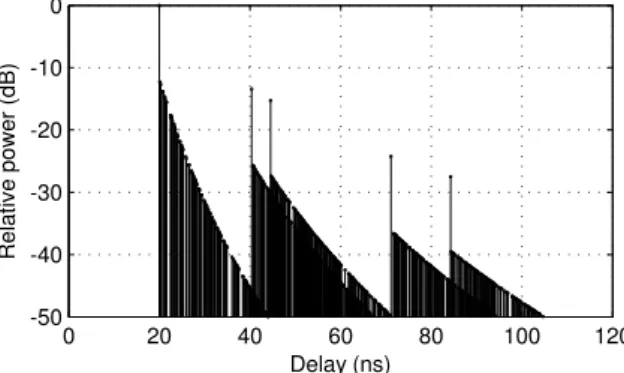
0 20 40 60 80 100 120 -50 -40 -30 -20 -10 0 Delay (ns) R e la ti v e p o w e r (d B )

Figure 8. CIR simulated over an infinite bandwidth. LOS situation, with the parameters d = 6 m, Λ = 36.5 MHz, λ = 5.95 GHz, Ω = 4.4, ω = 11.1 et G = 12 dB.

4.2. CIR Model over an Infinite Bandwidth

The principle of our UWB CIR model consists in generating the set of rays constituting the CIR while reproducing the characteristics observed during our experimental measurements. Among these characteristics, we mainly target at reproducing the clustering of multipath echoes, the ray and cluster arrival rates, and the decreasing magnitude of the PDP. For a baseband representation, a ray is described by its delay τ , its amplitude β and its phase θ. By generating these parameters, it is possible to describe the CIR over an infinite bandwidth. We then use these parameters in the frequency domain in order to include the effect of the limited observation bandwidth.

Our description of the CIR h(τ ) simulated over an infiinite frequency bandwidth follows the formalism of Saleh and Valen-zuela described in Eq. (4). As we experimentally observed in Section 3.4.1, the inter-cluster duration follows an exponential distribution. Thus, the arrival of a new cluster may be modelled by a Poisson process and the number of clusters in the CIR may be generated using a random variable L having the following law [5] :

pL(L) =

( ¯L)L_{exp(− ¯L)}

L! (8)

where ¯L represents the average number of clusters.

Having selected a Tx-Rx distance d for the simulation, the ToA of the first cluster is given by T1 = d_c, where c is the

speed of light. We then compute the ToA Tlof the L − 1 remaining clusters by generating inter-cluster durations following an

exponential law [15] :

p (Tl|Tl−1) = Λ exp (−Λ (Tl− Tl−1)) (9)

We observed that the inter-cluster power decay could be accurately fitted to a power function. (cf. Section 3.3). This approach differs from the one followed by Saleh and Valenzuela [15], but presents a closer fit to the experimental measurements. The amplitude of the first ray within each cluster is thus given by :

β1,l2 = β 2 1,1 „ Tl T1 «−Ω (10) where Ω represents the inter-cluster power decay constant.

In a second step, rays are iteratively generated for each cluster. The ToA of each ray is computed using inter-ray durations following an exponential law [15] :

p (τk,l|τk,l−1) = λ exp (−λ (τk,l− τk,l−1)) (11)

As we described in Section 3.3, a power function is used to compute the rays amplitude as :

βk,l2 = 10 −G 10_β2 1,l „ τk,l+ Tl Tl «−ω (12) where ω represents the intra-cluster power decay constant and G accounts for the observed attenuation between the first path of each cluster and the following multipaths. For each cluster, the generation of rays stops when the ray amplitude reaches a given threshold D, fixed at -50 dB in our simulations.

Finally, the phase θk,lof each ray is generated using an uniform law over the interval [0, 2π[. Figure 8 presents the rays

ob-tained in a LOS situation for a Tx-Rx distance of 6 m, where we may observe 5 clusters. It may be noted that this representation corresponds to an infinite observation bandwidth, each ray being represented by a Dirac function.

Table 3 summarizes all experimental parameters used in our statistical model of the UWB channel. 7

LOS NLOS ¯ L 5.6 2.4 Λ (MHz) 36.5 24.9 λ (GHz) 5.95 6.19 Ω 4.4 3.9 ω 11.1 10.2 G (dB) 12 0 Table 3

Parameters of the UWB channel model.

0 20 40 60 80 100 120 -130 -120 -110 -100 -90 -80 -70 -60 Delay (ns) R e la ti v e p o w e r (d B ) 0 20 40 60 80 100 120 -130 -120 -110 -100 -90 -80 -70 -60 Delay (ns) R e la ti v e p o w e r (d B ) (a) (b)

Figure 9. CIRs observed over limited bandwidths. Identical set of rays, observed over the 3.1 GHz - 10.6 GHz band (a) and the 3.1 GHz - 4.1 GHz band (b).

4.3. CIR Model over an Limited Bandwidth

In practice, the CIR is observed on a limited bandwidth, situated within the band 3.1 GHz - 10.6 GHz. We note fminand

fmaxthe minimum and maximum frequencies in the observation band, and fc= 1₂(fmin+ fmax) the center frequency. The CTF

limited to the observation bandwidth hence writes (for positive frequencies) :

Tlim(f ) = 8 < : fc f P L(fc,d) PL l=1 PKl k=1β 2 k,l PL l=1 PKl k=1βk,le j(θk,l−2πf (Tl+τk,l)) _iff min≤ f ≤ fmax 0 else (13)

where the coefficient P L(fc,d)

PL l=1 PKl k=1β 2 k,l

normalizes the power received at the frequency fcaccording to our path loss model.

In addition, the term fc

f accounts for the power decrease in −20 log(f ) described in Section 3.1. This CTF normalization

procedure was also proposed in [4] and [8].

The CIR observed over a limited bandwidth hlim(τ ) is simplu obtained from the CTF Tlim(f ) using an inverse Fourier

transform. In order to limit the side lobes level, it is possible to use a Hanning window for instance at this stage [24]. Figure 9 (a) represents our CIR example observed over the 3.1 GHz - 10.6 GHz frequency band. One may note that the low delay between two consecutive rays (cf. Fig. 8) naturally induces constructive or destructive interferences. Figure 9 (b) presents the same CIR observed over the 3.1 GHz - 4.1 GHz frequency band : one may note that the multipath resolution is less accurate when the observation bandwidth decreases.

4.4. Simulation Results

A series of simulations was conducted using the UWB radio channel model presented in Section 4. A set of 119 PDPs was generated using the same Tx-Rx distances as in our measurement campaign, for the LOS and NLOS situations. Each PDP was computed from a set of 90 CIRs, simulating the displacement of the antennas around a circle of 20 cm in diameter. The generation of the fast fading characteristics for the 90 locally simulated CIRs was performed using a geometrical algorithm, taking the ray angle of arrival into account. This algorithm is fully described in [12].

Figure 10 presents two typical PDPs obtained by simulation. One of the 90 constituting CIR is also represented. Note that on the x-axis, the delay was converted in path length. As a general observation, simulations are similar to the measured PDPs (cf. figure 3).

Two parameters representative of the channel temporal dispersion were computed for the entire set of generated PDPs : the

delay spread τRM S and the 75% delay window W75%. The average values obtained for these parameters in measurement

and simulation are compared for the LOS and NLOS situations in Table 4. One may note that the proposed model correctly reproduces the dispersion parameters experimentally measured over the UWB radio channel. The delay spread of the simulated PDPs is particularly close to the measurement, in both LOS and NLOS configurations. The values obtained for the delay window are somewhat different from the experimental data, but stay in the same range as the measured characteristics. The proposed model hence allows to reproduce not only the CIR structure, but also the channel dispersion.

0 10 20 30 40 50 60 70 -50 -40 -30 -20 -10 0 Delay (ns) R e la ti v e p o w e r (d B ) RI PDP 0 10 20 30 40 50 60 70 -50 -40 -30 -20 -10 0 Delay (ns) R e la ti v e p o w e r (d B ) RI PDP (a) (b)

Figure 10. PDPs and CIRs obtained by simulation. LOS (a) and NLOS (b) configurations.

LOS NLOS

Parameter Measurement Simulation Measurement Simulation

τRM S(ns) 4.1 4.0 9.9 9.7

W75%(ns) 7.6 9.7 23.7 21.2

Table 4

Comparison of the dispersion parameters : measurement vs. simulation.

5. Conclusion

In this paper, a complete study of the UWB propagation chanel is performed for the indoor office environment. The ac-quisition of over 10 000 CIRs in both LOS and NLOS configurations permits the assessment of the main UWB channel

char-acteristics. In a first step, we extract the path loss parameters N , σS and P L(f0, d0). We then analyse the main wideband

parameters for the UWB channel, such as the delay spread τRM Sand the arrival rates for the clusters Λ and rays λ. In

par-ticular, we propose a modification to the traditional Saleh and Valenzuela approximation for the PDP amplitude decay. Two original parameters, Ω and ω, are introduced to model the inter- and intra-cluster decay according to power functions.

From these experimental characteristics, we propose a complete UWB channel model. As a first step, we describe a path loss model, which may be used for network dimensioning studies and the assessment of interferences generated by UWB terminals. We also propose a detailed statistical model for the UWB CIR. This model generated a set of rays reproducing the characteristic structure of the CIR, such as the clustering of multiple propagation echoes. By filtering the set of generated rays, one may observe the CIR over any frequency band included within the 3.1 GHz - 10.6 GHz band. Simulations provided using this model show that the dispersion introduced by the radio channel is adequately reproduced. This model may thus be used for the realistic simulation of communication systems based on the UWB technology. Our futur research work wil address practical implementation issues, such as the integration of the model in a simulation tool with a minimized complexity.

References

[1] L. Yang and G. B. Giannakis, “Ultra-wideband communications: an idea whose time has come,” IEEE Signal Processing Magazine, vol. 21, no. 6, pp. 26–54, Nov. 2004.

[2] FCC, “First report and order, revision of Part 15 of the Commission’s rules regarding ultra-wideband transmission systems,” FCC, Tech. Rep. ET Docket 98-153, April 2002.

[3] A. F. Molisch, “Ultrawideband Propagation Channels - Theory, Measurement, and Modeling,” IEEE Transactions on Vehicular Technology, vol. 54, no. 5, pp. 1528–1545, Sept. 2005.

[4] J. Foerster, “Channel Modeling Sub-comitee Report Final,” IEEE P802.15 Working Group for WPANs, Tech. Rep. IEEE P802.15- 02/490r1-SG3a, Feb. 2003. [5] A. F. Molisch, K. Balakrishnan, C. C. Chong et al., “IEEE 802.15.4a channel model - final report,” IEEE 802.15 Working Group for WPANs, Tech. Rep. IEEE

P802.15-04/0662, Nov. 2004.

[6] J. Kunisch and J. Pamp, “Measurement results and modelling aspects for the UWB radio channel,” in IEEE Conference on Ultra Wide Band Systems and Technologies, Baltimore, MD, USA, May 2002, pp. 19–23.

[7] R. M. Buehrer, W. A. Davis, A. Safaai-Jazi et al., “Characterization of the ultra-wideband channel,” in IEEE Conference on Ultra Wide Band Systems and Technologies, Reston, VA, USA, Nov. 2003, pp. 26–31.

[8] A. Alvarez, G. Valera, M. Lobeira et al., “New channel impulse response model for UWB indoor system simulations,” in IEEE Vehicular Technology Conference, VTC Spring, vol. 1, Seoul, Korea, April 2003, pp. 1–5.

[9] D. Cassioli and A. Durantini, “Statistical characterization of UWB indoor propagation channels based on extensive measurement campaigns,” in International Symposium on Wireless Personal Multimedia Communications, vol. 1, Abano Terme, Italy, Sept. 2004, pp. 236–240.

[10] J. Karedal, S. Wyne, P. Almers et al., “UWB channel measurements in an industrial environment,” in IEEE Global Telecommunications Conference, vol. 6, Dallas, TX, USA, Nov. 2004, pp. 3511–3516.

[11] K. Haneda, J. Takada, and T. Kobayashi, “On the Cluster Properties in UWB Spatio-Temporal Residential Measurement,” in COST 273 Workshop, Bologna, Italy, Jan. 2005.

[12] P. Pagani, “Caractérisation et modélisation du canal de propagation radio en contexte Ultra Large Bande,” Ph.D. dissertation (in French), Institut National des Sciences Appliquées de Rennes, France, Nov. 2005.

[13] ITU, “Propagation prediction methods for the planning of ultra-wideband applications in the frequency range 1 GHz to 10 GHz (draft recommendation),” International Telecommunications Union, Tech. Rep. 3K/TEMP/18-E, Oct. 2004.

[14] S. S. Ghassemzadeh, L. J. Greenstein, A. Kavcic et al., “UWB indoor delay profile model for residential and commercial environments,” in IEEE Vehicular Technology Conference,VTC Fall, vol. 5, Orlando, FL, USA, Oct. 2003, pp. 3120–3125.

[15] A. A. M. Saleh and R. A. Valenzuela, “A Statistical Model for Indoor Multipath Propagation,” IEEE Journal on Selected Areas in Communications, vol. 5, no. 2, pp. 128–137, Feb. 1987.

[16] J. Karedal, S. Wyne, P. Almers et al., “Statistical Analysis of the UWB Channel in an Industrial Environment,” in IEEE Vehicular Technology Conference, VTC Fall, vol. 1, Los Angeles, CA, USA, Sept. 2004, pp. 81–85.

[17] D. Cassioli, M. Z. Win, and A. F. Molisch, “The ultra-wide bandwidth indoor channel: from statistical model to simulations,” IEEE Journal on Selected Areas in Communications, vol. 20, no. 6, pp. 1247–1257, Aug. 2002.

[18] J. Kunisch and J. Pamp, “An ultra-wideband space-variant multipath indoor radio channel model,” in IEEE Conference on Ultra Wide Band Systems and Technologies, Reston VA, USA, Nov. 2003, pp. 290–294.

[19] S. M. Yano, “Investigating the Ultra-Wideband Indoor Wireless Channel,” in IEEE Vehicular Technology Conference, VTC Spring, vol. 3, Birmingham, AL, USA, May 2002, pp. 1200–1204.

[20] R. J. M. Cramer, R. A. Scholtz, and M. Z. Win, “Evaluation of an ultra-wide-band propagation channel,” IEEE Transactions on Antennas and Propagation, vol. 50, no. 5, pp. 561–570, May 2002.

[21] B. Denis and J. Keignart, “Post-processing framework for enhanced UWB channel modeling from band- limited measurements,” in IEEE Conference on Ultra Wide Band Systems and Technologies, Reston, VA, USA, Nov. 2003, pp. 260–264.

[22] A. Abdi and M. Kaveh, “Performance comparison of three different estimators for the Nakagami m parameter using Monte Carlo simulation,” IEEE Communications Letters, vol. 4, no. 4, pp. 119–121, April 2000.

[23] U. Schuster, “Indoor UWB Channel Measurements from 2 GHz to 8 GHz,” IEEE 802.15 Working Group for Wireless Personal Area Networks (WPANs), Tech. Rep. IEEE 802.15-04/447, Sept. 2004.

[24] F. J. Harris, “On the Use of Windows for Harmonic Analysis with the Discrete Fourier Transform,” Proceedings of the IEEE, vol. 66, no. 1, pp. 51–83, Jan. 1978.