HAL Id: hal-01896654
https://hal-imt-atlantique.archives-ouvertes.fr/hal-01896654
Submitted on 16 Oct 2018
HAL is a multi-disciplinary open access
archive for the deposit and dissemination of
sci-entific research documents, whether they are
pub-lished or not. The documents may come from
teaching and research institutions in France or
abroad, or from public or private research centers.
L’archive ouverte pluridisciplinaire HAL, est
destinée au dépôt et à la diffusion de documents
scientifiques de niveau recherche, publiés ou non,
émanant des établissements d’enseignement et de
recherche français ou étrangers, des laboratoires
publics ou privés.
Spatio-Temporal Interpolation of Satellite-derived Sea
Surface Temperature
Said Ouala, Ronan Fablet, Cédric Herzet, Bertrand Chapron, Ananda
Pascual, Fabrice Collard, Lucile Gaultier
To cite this version:
Said Ouala, Ronan Fablet, Cédric Herzet, Bertrand Chapron, Ananda Pascual, et al..
Neural-Network-based Kalman Filters for the Spatio-Temporal Interpolation of Satellite-derived Sea Surface
Temper-ature. Remote Sensing, MDPI, 2018, 10 (12), pp.1864. �10.3390/rs10121864�. �hal-01896654�
Neural-Network-based Kalman Filters for the
Spatio-Temporal Interpolation of Satellite-derived
Sea Surface Temperature
Said Ouala1* , Ronan Fablet2, Cédric Herzet3, Bertrand Chapron4, Ananda Pascual5, Fabrice Collard6, Lucile Gaultier7
1 IMT Atlantique, Lab-STICC, UBL, Brest, France; [email protected] 2 IMT Atlantique, Lab-STICC, UBL, Brest, France; [email protected]
3 IMT Atlantique, Lab-STICC, UBL, Brest; INRIA Bretagne-Atlantique, SIMSMART, Rennes, France; [email protected]
4 Ifremer, LOPS, Brest, France; [email protected]
5 IMEDEA, UIB-CSIC, Esporles, Spain; [email protected] 6 ODL, Brest, France; [email protected]
7 ODL, Brest, France; [email protected]
* Correspondence: [email protected] Version October 15, 2018 submitted to Remote Sens.
Abstract:In this work we address the reconstruction of gap-free Sea Surface Temperature (SST) fields
1
from irregularly-sampled satellite-derived observations. We develop novel Neural-Network-based
2
(NN-based) Kalman filters for spatio-temporal interpolation issues as an alternative to ensemble
3
Kalman filters (EnKF). The key features of the proposed approach are two-fold: the learning of
4
a probabilistic NN-based representation of 2D geophysical dynamics, the associated parametric
5
Kalman-like filtering scheme for a computationally-efficient spatio-temporal interpolation of Sea
6
Surface Temperature (SST) fields. We illustrate the relevance of our contribution for an OSSE
7
(Observing System Simulation Experiment) in a case-study region off South Africa. Our numerical
8
experiments report significant improvements in terms of reconstruction performance compared with
9
operational and state-of-the-art schemes (e.g., optimal interpolation, Empirical Orthogonal Function
10
(EOF) based interpolation and analog data assimilation).
11
Keywords: Data assimilation; Dynamical model; Kalman filter; Neural networks; Data-driven
12
models; Interpolation
13
1. Introduction
14
Satellite sensors and in-situ networks can provide observations of sea surface tracers (e.g.
15
temperature, salinity, ocean colour). However, due to sensors’s characteristics (e.g., space-time
16
sampling, sensor type) and their sensitivity to the atmospheric conditions (e.g., rain, clouds), only
17
partial and possibly noisy observations are available. As a consequence, no sensor can provide gap-free
18
high-resolution observations in space and time. A typical example of the missing data pattern for SST
19
is reported in Fig.3for an infrared sensor. In some situations, missing data may become very large
20
which makes crucial the development of spatio-temporal interpolation tools.
21
Within the satellite ocean community, Optimal interpolation (OI) is the standard technique [1–7].
22
Given a covariance model of spatio-temporal dynamics, the interpolated field results from a linear
23
combination of the observations. The parameters of the linear combination are typically tuned by
24
exploiting some statistical properties of the target field.
25
In general, stationary covariance hypotheses are considered, which prove relevant for the
26
reconstruction of horizontal scales above 100km. Fine scale components may hardly be retrieved
27
with such approaches and a variety of research studies aim to improve the reconstruction of the
28
high-resolution component of our spatio-temporal fields.
29
Empirical Orthogonal Function (EOF) based interpolation is an other categorie widely used in
30
geosciences [8–10]. They rely on a Singular Value Decomposition (SVD) to compute the EOF basis, the
31
field is then reconstructed by projecting the observations on the EOF subspace until a convergence
32
criterion is reached [11]. Unfortunately, dealing with high missing data rates decreases the encoded
33
variability in the EOF components witch results in smoothing fine scale components.
34
Data assimilation is the state-of-the-art framework for the reconstruction of dynamical systems
35
from partial observations based on a given numerical model [12,13]. Statistical data assimilation
36
schemes especially ensemble Kalman filters, have become particularly popular due to their trade-off
37
between computational efficiency and modeling flexibility. Unlike OI and EOF based techniques,
38
these schemes explicitly rely on dynamical priors to address interpolation issues from partial and
39
noisy observations. When dealing with sea surface dynamics, the analytical derivation of these
40
priors involves simplifying assumptions which may not be satisfied by real observations. By contrast,
41
realistic analytical parameterizations may lead to highly computationally-demanding numerical
42
models associated with modeling and inversion uncertainties, which may limit their relevance for an
43
application of the interpolation of a single sea surface tracer.
44
Recently, data-driven approaches [8,14] have emerged as relevant alternatives to model-driven
45
schemes. They take benefit from the increasing availability of remote sensing observation and
46
simulation data to derive dynamical priors from these datasets. Analog methods are one of the first
47
data-driven techniques to develop this data-driven paradigm within a data assimilation framework
48
[14]. Analog forecasting operators provide a data-driven formulation of the dynamical operator, which
49
can be used as a plug-and-play operator in Kalman-based assimilation schemes. Combined with
50
patch-based representation, the analog data assimilation was recently proven to be relevant with
51
respect to OI and EOF-based schemes for the spatio-temporal interpolation of sea surface geophysical
52
tracers [15–17].
53
In this paper, we further investigate data-driven interpolation approaches within a statistical
54
data assimilation framework. We focus on neural network and deep learning models, which have
55
rapidly become the state-of-the-art in machine learning for a wide range of applications, including
56
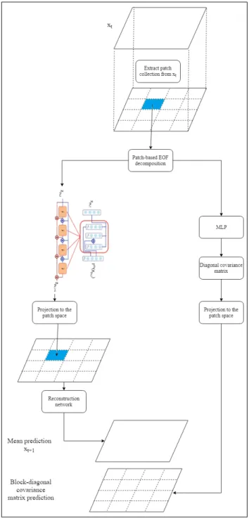
inverse imaging issues [18]. Recent applications to the assimilation of low-dimensional dynamical
57
systems [19] and to the forecasting of geophysical dynamics [20] have been developed. However,
58
to our knowledge, the design of neural-network-based assimilation models for the spatio-temporal
59
interpolation of geophysical dynamics remain an open challenge, which may greatly benefit from the
60
ability of deep learning models to capture computationally-efficient representations from available
61
ocean observation and simulation datasets. In this study, we address this challenge and propose a novel
62
NN-based Kalman filtering scheme applied to the spatio-temporal interpolation of satellite-derived
63
sea surface temperature. We exploit a ResNet architecture [19,21] and a patch-based decomposition
64
[22] to derive a data-driven representation of spatio-temporal fields. Importantly, this architecture
65
conveys a probabilistic representation through the prediction of a mean component and a covariance
66
pattern. The later may be regarded as a NN-based representation of the covariance patterns issued
67
from Monte Carlo approximations in ensemble assimilation schemes [23]. Overall, the methodological
68
contributions of this work are two-fold: i) we propose a new probabilistic NN-based representation
69
of 2D geophysical dynamics, ii) we derive the associated NN-based Kalman filtering scheme for
70
spatio-temporal interpolation issues. We demonstrate the relevance of these contributions with respect
71
to state-of-the-art approaches [2,8,16] for the spatio-temporal interpolation of satellite-derived SST
72
fields in a case study region off South Africa. This paper is organized as follows. Section2reviews
73
data assimilation schemes. Section3describes the proposed neural-network-based data assimilation
framework. Section4presents the results of the numerical experiments. We further discuss our
75
contributions in Section6.
76
2. Problem statement and related work
77
Regarding ocean remote sensing data, spatio-temporal interpolation issues can be regarded as the
78
reconstruction of some hidden states from partial and/or noisy observation series, referred to as data
79
assimilation in geoscience [23]. Data assimilation techniques usually involve a state-space evolution
80
model [23]:
81
xt+1= F (xt) +ηt (1)
yt+1= H(xt+1) +et (2)
where t∈ {0, ..., T}represents the temporal resolution of our time series andF the dynamical
82
model describing the temporal evolution of the physical variables x. The observation modelHlinks the
83
observation y to the physical variable x. ηtand etare random processes accounting for the uncertainties
84
in the dynamical and observation models. They are usually defined as centered Gaussian processes
85
with covariances Qtand Rtrespectively.
86
From a probabilistic point of view, the spatio-temporal interpolation problem can be seen
87
as a Bayesian filtering problem where the main goal is to evaluate the conditional probabilities
88
p(xt+1|y1, ..., yt) (prediction distribution of the state xt+1 given observations up to time t) and
89
p(xt+1|y1, ..., yt, , yt+1) (posterior distribution of xt+1 given observations up to time t+1). Under
90
certain assumptions over the state space model (the dynamical and observation models are linear
91
with Gaussian uncertainties), the prediction and posterior distributions are also Gaussian and can be
92
written as :
93
p(xt+1|y1, ..., yt) = N (xt+1− ,Σ−t+1) (3) p(xt+1|y1, ..., yt+1) = N (xt+1+ ,Σ+t+1) (4) with the means and covariances computed for each time t using the well known Kalman recursion
94 x−t+1=Fx+t (5) Σ− t+1=FΣ + t FT+Qt (6) x+t+1=x−t+1+Kt+1[yt+1−Ht+1x−t+1] (7) Σ+ t+1=Σ − t+1−Kt+1Ht+1Σ−t+1 (8) with 95 Kt+1 =Σ−t+1Ht+1T [Ht+1Σ−t+1Ht+1T +Rt]−1. (9) Here F and Ht+1corresponds respectively to some linear dynamical and observation models. The
96
superscript (-) refers to the forecasting of the mean of the state variable x−t+1and of its covariance matrix
97
Σ−
t+1given observations up to time t but without the new observation at time t+1. The superscript (+)
98
refers in the other hand to the mean of the state variable x+t+1and of the covariance matrixΣ+t+1given
99
all observations up to time t+1. They are referred to as the assimilated mean and covariance. Kt+1is
100
the Kalman gain. Kalman filters provide a sequential formulation of the Optimal Interpolation (OI)
101
[24] which may also be solved directly knowing the space-time covariance of processes x and y. For
non-linear and high-dimensional dynamical systems, the pdfs are not Gaussian anymore and the above
103
Kalman recursion does define their means and covariances. Ensemble Kalman methods have been
104
proposed to address these issues. The ensemble Kalman filter and smoother [23] are the first sequential
105
filtering techniques used reliably in the reconstruction of geophysical fields. The key idea here is to
106
approximate the forecasting mean x−t+1and covarianceΣ−t+1by a sample mean and covariance matrix
107
computed by propagating an ensemble of M members,{xi−t+1}M
i=1, using the dynamical modelF.
108 xi−t+1= F (xi+t , i∈ {0, ..., N}) (10) Σ− t+1= 1 N−1Dt+1D t t+1 (11) Dt+1= [x1−t+1−x−t+1, ...xN−t+1−x−t+1] (12) xi+t+1=xi−t+1+Kt+1[yt+1−Ht+1xi−t+1] (13) Kt+1=Σ−t+1Ht+1T [Ht+1Σ−t+1Ht+1T +Rt]−1 (14) Σ+
t+1=Σ −
t+1−Kt+1Ht+1Σ−t+1 (15)
Besides all its advantages, EnKF techniques do not escape the curse of dimensionality.
109
High-dimensional systems require using large ensemble sizes M which may lead to very
110
high-computational complexity. The use of small ensemble sizes in the other hand may result in
111
undersampling the covariance matrix (the considered ensemble is not representative of our systems
112
dynamics) which may in turn result in poor reconstruction performance, including for instance
113
filter divergence and spurious long-range correlations. Proposed solutions such as inflation [25],
114
cross-validation [26] and localization methods[27–29] may require thorough tuning experiments.
115
An alternative strategy based on a model-driven propagation of parametric covariance models
116
[30,31] seems appealing. Using advection priors [32], it propagates parametric covariance structures,
117
which leads to the implementation of the classic Kalman recursion. Accounting for more complex
118
dynamical priors for the covariance structure is an open question, which may limit the applicability
119
of this approach to complex geophysical systems. Inspired by the later parametric framework,
120
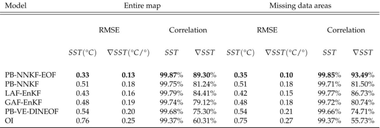
we aim to design an efficient sequential filtering technique for the reconstruction of geophysical
121
fields. Rather than considering a model-driven prior to propagate Gaussian states as in [30,31], we
122
investigate NN-based priors, which may be fitted from training data. The resulting NN-based Gaussian
123
representations provide computationally-efficient approximations of the dynamical priors that should
124
prevent undersampling issues within a Kalman recursion.
125
3. Proposed interpolation model
126
3.1. Neural-network Gaussian dynamical prior
127
Our key idea is to exploit neural-network (NN) representations for the time propagation of
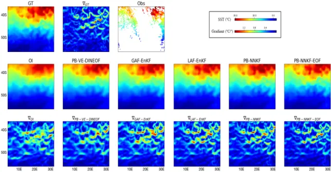
128
a Gaussian approximation of the distribution of the state. Compared with dynamical priors in
129
assimilation model (1), which state conditional distribution xt|xt−1, we here consider neural-network
130
representations to extend the prediction step of the Kalman recursion (5-6) to non-linear dynamics.
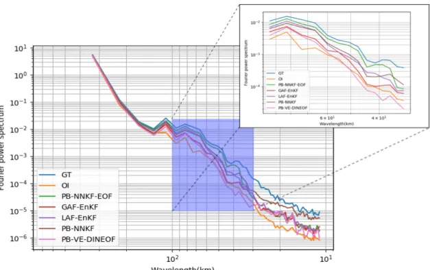
131
Formally, it comes to define:
132
x−t+1= F (xt+) (16)
Σ−
t+1= FΣ(x+t ,Σ+t ) (17) with x−t+1andΣ−t+1the mean and covariance of the prediction of the Gaussian approximation
133
of the state at time t+1 given the assimilated mean x+t and covariance Σ+t at time t. Functions
134
F,FΣare neural networks to be defined with parameter vectors θ= (θµ, θΣ). It may noted that our
parameterization follows (5-6) such that the update of the mean component in (16) only depends on
136
the mean at the previous time step and the update of the covariance depends both on the mean and
137
covariance at the previous time step. Given this NN-based representation of the prediction step of the
138
Kalman filter, we apply the classic Kalman-based filtering under the assumption that the observation
139
model is linear and Gaussian:
140
x+t+1=x−t+1+Kt+1[yt+1−Ht+1x−t+1] (18) Kt+1=Σ−t+1HTt+1[Ht+1Σ−t+1Ht+1T +Rt]−1 (19) Such a formulation does not require forecasting an ensemble to compute a sample covariance
141
matrix. It results in a significant reduction of the computational complexity. The same holds when
142
compared to the computational complexity of the analog data assimilation which involves ensemble
143
forecasting and repeated nearest-neighbor search.
144
3.2. Patch-based NN architecture
145
When considering spatio-temporal fields, the application of the model defined by (16) and
146
(17) should be considered with care to account for the underlying dimensionality, especially for the
147
covariance model in (19). Following our previous works on analog data assimilation [15,16], we
148
consider a patch-based representation1. This patch-based representation is fully embedded in the
149
considered NN architecture to make explicit both the extraction of the patches from a 2D field and the
150
reconstruction of a 2D field from the collection of patches. The later involves a reconstruction operator
151
which is learnt from data.
152
Regarding modelF, the proposed architecture proceeds as follows:
153
• At a given time t, the first layer of the network, which is parameter-free in terms of training,
154
comes to decompose an input field xt into a collection of Np P×P patches xPs,t, where P is
155
the width and height of each patch and s the patch location in the global field. Each patch is
156
decomposed onto an EOF basisBaccording to :
157
zPs,t=xPs,tB
T (20)
with zPs,tthe EOF decomposition of the patch xPs,t. The EOF decomposition matrixBis trained
158
offline as preprocessing step;
159
• The second layer implements a numerical integration scheme (typically, an Euler or 4th-order
160
Runge-Kutta scheme) using a patch-level dynamical model FPs, s ∈ [1, ..., Np] to predict
161
zPs,t+1. For patch-level modelsFPs, we consider residual architectures [21] with a bilinear
162
parameterization [19];
163
• The third layer is a reconstruction network Fr. It combines the predicted patches xPs,t =
164
zPs,tB, s∈ [1, ..., Np]to reconstruct the output field xt. This reconstruction networkFrinvolves a
165
convolution neural network [33].
166
The details of the considered parameterizations for the second and third layers are given in
167
Section4. To train mean dynamical modelF, we apply a two-step procedure. We first learn the local
168
dynamical modelsFPs, s∈ [1, ..., Np]based on the minimization of the EOF-patch based forecasting
169
error. The reconstruction networkFris then optimized using the same criterion over the global field.
170
Regarding covariance modelFΣwe also consider a patch-based representation of the spatial
171
domainFPs
Σ , more precisely a block-diagonal parameterization of the patch-level covariances in the
172
EOF space. It may be noted that a diagonal parameterization of the covariance in the EOF space forms
173
a full covariance matrix in the original patch space. This block-diagonal covariance modelFΣis learnt
174
separately for each patch according to a ML (Maximum Likelihood) criterion. The associated training
175
dataset comprises patch-based EOF decompositions of the forecasted states according to the mean
176
modelFPs from states of the training dataset corrupted by an additive Gaussian perturbation with a
177
covariance structureΣ0. Here,Σ0is given by the empirical covariance of the EOF patches for the entire
178
training dataset. Overall, for a given patchPs, we parameterizeFPs
Σ the restriction of covarianceFΣ
179
onto patchPsas:
180 FPs Σ (xPs,t+1,ΣPs,t+1) = B tΨ(Σ Ps,t,Σ0) · F Ps D(zPs,t,Σ0) · B (21)
withΨ(ΣPs,t−1,Σ0)a scaling function. Among different parameterizations, a constant scaling
181
functionΨ() =1 led to the best performance in our numerical experiments.
182
To illustrate the relevance of the proposed full covariance matrix parametrization (based on a
183
patch based projection on the EOF space and illustrated for instance by equation21), we also investigate
184
a diagonal covariance matrix model in the patch space.
185
3.3. Data assimilation procedure
186
Given a trained patch-based NN representation as described in the previous section, we derive
187
the associated Kalman-like filtering procedure. As summarized in Algorithm1, at time step t, given the
188
Gaussian approximation of the posterior likelihood P(xt−1|y0, . . . , yt−1)with mean x+t−1and covariance
189
Σ+
t−1, we first compute the forecasted Gaussian approximation at time t with mean fieldF (x + t−1)and
190
patch-based covarianceFΣ(x+t−1,Σ+t−1). The assimilation of the new observation ytis performed at
191
a patch-level. For each patchPs, we update the patch-level mean x+P
s,tand covarianceΣ
+
Ps,tusing
192
Kalman recursion (8) with observation yPs,t. We then combine these patch-level updates to obtain
193
global mean x+t and covarianceΣ+t . Whereas we compute global mean x+t using trained reconstruction
194
networkFr,Σ+t just comes to store the collection of patch-level covariances. This procedure is iterated
195
up to the end of the observation sequence.
196
Compared with the patch-based analog data assimilation [16], it might be noted that we iterate
197
patch-level assimilation steps and global reconstruction steps thanks to the NN-based propagation of
198
the patch-based covariance structure. This procedure potentially allows information propagation from
199
one patch to neighborhing ones after each assimilation step. By contrast, in the patch-based analog
200
data assimilation, each patch is processed independently, such that no such information propagation
201
can occur. This is regarded as a key feature to account for the propagation of geophysical structures
202
(e.g., fronts, eddies, filaments,...).
203
We refer to the patch-based NNKF reconstruction model using the EOF block-diagonal
204
parameterization of the covariance modelFΣ, as model PB-NNKF-EOF. The model using the diagonal
205
parameterization of the covariance modelFΣin the patch space is referred to as PB-NNKF.
206
4. Data and experimental setting
207
As a case-study, we address the spatio-temporal interpolation of satellite-derived SST fields
208
associated with infrared sensors, which may involve high missing data rates (typically from 50% to
209
90%). We consider the same region and dataset as in [16] to make easier benchmarking analyses.
210
4.1. Dataset description
211
As SST time series used here is delivered by the UK Met Office [2] from January 2008 to December
212
2015. The spatial resolution of our SST field is 0.05° and the temporal resolution h=1 day. The data
213
from 2008 to 2014 were used as training data and we tested our approach on the 2015 data. To perform
Figure 1. Proposed neural-network-based representation of a spatio-temporal dynamical system. The
input Xtis first decomposed into P×P patches, each patch is then propagated using its associate local dynamical model. The output Xt+1is then reconstructed by injecting the forecasted patches into the reconstruction model
Algorithm 1Patch-based NNKF reconstruction 1: procedurePB-NNKF(F,FΣ,y,R) 2: for t in[0, ..., T]: 3: x−t ← F (x+t−1) 4: [Σ−P 0,t, ...,Σ − PNp,t] ← FΣ(x + t−1,Σ + t−1) 5: [x−P 0,t, ..., x − PNp,t] ←ExtractPatches(x − t ) 6: [yP0,t, ..., yPNp,t] ←ExtractPatches(yt) 7: for s in[1, ..., Np]: 8: KPs,t=Σ−Ps,tH t Ps,t[HPs,tΣ − Ps,tH t Ps,t+Rt] −1 9: XP+s,t=x−Ps,t+KPs,t[yPs,t−HPs,tx − Ps,t] 10: Σ+P s,t=Σ − Ps,t−KPp,tHPp,tΣ − Pp,t 11: x+t ←Reconstruct([x+P 0,t, ..., x + PNs,t]) 12: Σ+t ←Reconstruct([Σ+P 0,t, ...,Σ + PNs,t])
a quantitative evaluation, we simulated realistic spatio-temporal cloud patterns using METOP-AVHRR
215
masks. This sensor is highly sensitive to the cloud cover and results in very high missing data rates
216
as illustrated in Fig. 3. As case-study area, we select an area off South Africa (from 2.5°E, 38.75°S
217
to 32.5°E, 58.75°S). This region involves complex fine-scale SST dynamics (e.g., fronts, filaments). It
218
makes it relevant for the considered quantitative evaluation.
219
4.2. Experimental setting
220
The proposed neural-network-based Kalman scheme involves the following parameter setting.
221
The proposed patch-based and NN-based Kalman filter is applied to SST anomaly fields w.r.t.
222
optimally-interpolated SST fields (see below for the parameterization of the optimal interpolation).
223
These optimally-interpolated fields provide a relevant reconstruction of horizontal scales up to≈100km.
224
We exploit patch-level representations with non-overlapping 20×20 patches. For each patchPs, we
225
learn an EOF basis from the training data. We keep the first 50 EOF components, which amount on
226
average to 95% of the total variance. For the patch-level NN modelFPs, we use a bilinear residual
227
neural network architecture as proposed in [34] with 60 linear neurons, 100 bilinear neurons and 10
228
fully-connected layers with a Relu activation. The reconstruction modelFris a convolutional neural
229
network with 3 convolutional layers. The first two layers comprise 64 filters of size 3×3 with a Relu
230
activation and the last layer is a linear convolutional layer with one filter. Regarding covariance model
231
FPs
D , we consider a diagonal covariance model within each patch. Each element of diagonal involves
232
a a 3-layer MLP with 4 neurons and Relu activation functions on the hidden layers and a softplus
233
activation in the output layer. With a view to evaluating the EOF-based covariance parameterization,
234
we consider both PB-NNKF-EOF and PB-NNKF schemes.
235
We perform a quantitative analysis of the interpolation performance of the proposed scheme with
236
respect to an optimal interpolation, the analog data assimilation [16] and the EOF based interpolation
237
method VE-DINEOF. The considered parameter setting is as follows:
238
• Optimal interpolation (OI) : We use a Gaussian kernel with a spatial correlation length of 100km
239
and a temporal resolution length of 3 days. These parameters were empirically tuned for the
240
considered dataset using a cross-validation experiment.
241
• Analog data assimilation (LAF-EnKF, GAF-ENKF): We apply both the global and local analog
242
data assimilation schemes, referred to as G-AnDA and L-AnDA [14,16]. Similarly to the
243
proposed scheme, we consider 20×20 patches and 50-dimensional EOF decomposition with
244
an overlapping of 10 pixels. We let the reader refer to [14,16] for a detailed description of this
245
data-driven approach, which relies on nearest-neighbor regression techniques.
Figure 2. Selected patches on the high resolution component of the SST data. (The SST map corresponds
to July 19, 2015)
• EOF based reconstruction (PB-VE-DINEOF): We also compare our approach to the state-of-the-art
247
interpolation scheme based on the projection of our observations with missing data on an
248
EOF basis [8]. The SST field is here decomposed as described in the analog data assimilation
249
application into a collection of 20×20 patches with a 10 pixels overlapping. Each patch is then
250
reconstructed using the VE-DINEOF method.
251
5. Results and discussion
252
We report in this section the results of the considered numerical experiments. We first focus on
253
patch-level performance as the patch-based representation is at the core of the proposed interpolation
254
model. We then report interpolation performance for the whole case-study region.
255
5.1. Patch-level interpolation performance
256
We first evaluate the patch-level interpolation performance of the proposed scheme for four
257
patches corresponding to different dynamical modes as illustrated in Fig. 2located in the area (5°E
258
to 75°E and latitude 25°S to 55°S). In Tab.1, we report the interpolation performance in terms of
259
RMSE (root mean square error) for the proposed EOF NN-based scheme (NNKF-EOF) and include a
260
comparison to the local analog data assimilation (LAF-EnKF). With a view to specifically analyzing
261
the relevance of NN-based parametric covariance model, we also apply an ensemble Kalman filter
262
with the trained dynamical modelFPs. The reported results clearly illustrate the relevance of the
263
proposed NN-based scheme for the assimilation of a single patch. The proposed NN-based scheme,
264
which combines a NN-based formulation of the mean forecasting operator and of the associated
265
covariance pattern, slightly outperforms the ensemble Kalman filters, while also significantly reducing
266
the computational complexity induced by the generation of ensembles of size 500.
267
5.2. Global interpolation performance
268
We further evaluate the performance of the proposed schemes over the considered case-study
269
region. Tab.2report the mean forecasting RMS error of the proposed NN-based representation
270
compared with local and global forecasting operator [14]. The proposed patch-level NN-based model
271
outperforms the benchmarked approaches by about 5-15% in terms of interpolation RMSE, which
272
stresses the relevance of mean dynamical modelF.
273
We report the mean interpolation performance in Tab. 3and the time series of interpolation
274
errors illustrated in Fig.5. The proposed NN-based scheme (PB-NNKF-EOF) leads to very significant
275
improvements with respect to the optimal interpolation in terms of RMSE and correlation coefficients
276
for both the SST and its gradient, which emphasizes fine-scale structures (e.g., relative improvement of
Assimilation method Considered patch RMSE (°C)
Patch1 Patch2 Patch3 Patch4
LAF EnKF 0.50 0.25 0.22 0.39
Bi-NN-EnKF 0.55 0.23 0.22 0.30
Bi-NN-NNKF-EOF 0.46 0.20 0.19 0.27
Table 1. Patch-level interpolation experiment: RMSE of the reconstructed anomaly fields for the LAF EnKF
(local analog forecasting based ensemble Kalman filter), Bi-NN-EnKF (Bilinear residual neural net model (FPs)
used in an ensemble Kalman filter), Bi-NN-NNKF (Proposed NNKF based on a bilinear residual neural net dynamical mean model).
Figure 3. Interpolation of the SST field on July 19 2015: first row, the reference SST, its gradient and the
observation with missing data (here, 82% of missing data); second row, interpolation results using respectively OI, PB-VE-DINEOF, GAN-EnKF, LAN-ENKF, PB-NN-NNKF, PB-NN-NNKF-EOF; third row, gradient of the reconstructed fields.
the RMSE above 50% for missing data areas for the SST and its gradient). A clear gain is also exhibited
278
w.r.t. analog data assimilation and PB-VE-DINEOF schemes with a relative gain greater than 20% in
279
terms of RMSE for both the SST and its gradient. The same conclusion holds in terms of correlation
280
coefficients close to 90% or above for all parameters for PB-NNKF-EOF scheme, all the other ones
281
depicting correlation coefficients below 85% for SST gradient fields. Although the considered NN-based
282
representation exploits non-overlapping patches, we still come up with significant improvements w.r.t
283
AnDA schemes which involve a 50% overlapping rate between patches. This clearly illustrates the
284
relevance of NN-based representation, which fully embeds the direct and inverse mappings between
285
the SST field and its patch-level representation. Interestingly, Tab.3also reveals the importance of
286
the EOF-based parameterization of the NN-based covariance model (21) in the improvement of
287
interpolation results w.r.t. AnDA schemes.
288
We further illustrate these conclusions through interpolation examples in Fig. 3. The visual
289
analysis of the reconstructed SST gradient fields emphasize the relevance of PB-NNKF-EOF scheme to
290
reconstruct fine-scale details. While OI and PB-VE-DINEOF schemes tend to smooth out fine-scale
291
patterns, the analog data assimilation may not account appropriately for patch boundaries. This
292
typically requires an empirical post-processing step [16]. By contrast, the PB-NNKF-EOF scheme fully
293
embeds this post-processing step through reconstruction layerFrand learns its parameterization from
294
data, which is shown here to greatly improve patch-based interpolation performance. The analysis of
295
the spectral signatures leads to similar conclusions with the PB-NNKF-EOF scheme being the only one
296
to recover significant energy level up to 50km.
297
Model Forecasting RMSE (°C)
t+h t+4h t+8h
PB-NN 0.48 0.60 0.63
LAF 0.50 0.68 0.76 GAF 0.61 0.74 0.76
Table 2. Forecasting experiment for several prediction time steps
Model Entire map Missing data areas
RMSE Correlation RMSE Correlation
SST(°C) ∇SST(°C/°) SST ∇SST SST(°C) ∇SST(°C/°) SST ∇SST PB-NNKF-EOF 0.33 0.13 99.87% 89.30% 0.35 0.10 99.85% 93.49% PB-NNKF 0.51 0.18 99.75% 81.24% 0.51 0.18 99.71% 81.50% LAF-EnKF 0.43 0.16 99.79% 84.41% 0.42 0.15 99.77% 86.73% GAF-EnKF 0.48 0.19 99.74% 79.12% 0.48 0.18 99.72% 80.74% PB-VE-DINEOF 0.54 0.20 99.68% 75.30% 0.54 0.21 99.66% 74.71% OI 0.76 0.25 99.37% 60.31% 0.75 0.27 99.37% 55.73%
Table 3. SST interpolation experiment: Reconstruction correlation coefficient and RMSE over the SST time
series and their gradient.
6. Conclusion
298
In this work, we addressed neural-network-based models for the spatio-temporal interpolation
299
of satellite-derived SST fields with large missing data rates. We introduced a novel probabilistic
Figure 4. Radially averaged power spectral density of the interpolated SST fields with respect to the reference SST.
NN-based representation of geophysical dynamics. This representation, which relies on a patch-level
301
and EOF-based representation, allows us to propagate in time a mean component and the covariance
302
of the SST field. It makes direct the derivation of an associated Kalman filter for the spatio-temporal
303
interpolation of SST fields. Our numerical experiments stress a significant gain in interpolation
304
performance w.r.t. optimal interpolation and other state-of-the-art data-driven schemes, such DINEOF
305
[8] and analog data assimilation [14,16].
306
Further work could explore the application of the proposed framework to other sea surface
307
geophysical tracers, including multi-source and multi-modal interpolation issues. SLA (Sea Level
308
Anomaly) fields could provide an interesting case-study as the associated space-time sampling is
309
particularly scarce and multi-source strategies are of key interest [35].
310
Author Contributions:S.A, R.F. and C.H. stated the methodology; S.A., R.F., L.G., F.C., B.C and A.P. conceived
311
and designed the experiments; S.A. performed the experiments; L.G., F.C., B.C. and A.P. discussed the experiments;
312
R.L. and R.F. wrote the paper. B.C, A.P. and C.H. proofread the paper.
313
Funding:This work was supported by GERONIMO project (ANR-13-JS03-0002), Labex Cominlabs (grant SEACS),
314
Region Bretagne, CNES (grant OSTST-MANATEE), Microsoft (AI EU Ocean awards) and by MESR, FEDER,
315
Région Bretagne, Conseil Général du Finistère, Brest Métropole and Institut Mines Télécom in the framework of
316
the VIGISAT program managed by "Groupement Bretagne Télédétection" (BreTel).
317
References
318
1. Escudier, R.; Bouffard, J.; Pascual, A.; Poulain, P.M.; Pujol, M.I. Improvement of coastal and mesoscale
319
observation from space: Application to the northwestern Mediterranean Sea. Geophysical Research Letters
320
2013, 40, 2148–2153. doi:10.1002/grl.50324.
321
2. Donlon, C.J.; Martin, M.; Stark, J.; Roberts-Jones, J.; Fiedler, E.; Wimmer, W. The Operational Sea Surface
322
Temperature and Sea Ice Analysis (OSTIA) system. Remote Sensing of Environment 2012, 116, 140–158.
323
doi:10.1016/j.rse.2010.10.017.
324
3. Le Traon, P.Y.; Nadal, F.; Ducet, N. An improved mapping method of multisatellite altimeter data. Journal
325
of atmospheric and oceanic technology 1998, 15, 522–534.
326
4. Droghei, R.; Buongiorno Nardelli, B.; Santoleri, R. A New Global Sea Surface Salinity and Density Dataset
327
From Multivariate Observations (1993–2016). Frontiers in Marine Science 2018, 5, 84.
328
5. Nardelli, B.B.; Pisano, A.; Tronconi, C.; Santoleri, R. Evaluation of different covariance models for the
329
operational interpolation of high resolution satellite Sea Surface Temperature data over the Mediterranean
330
Sea. Remote Sensing of Environment 2015, 164, 334–343.
331
6. Ducet, N.; Le Traon, P.Y.; Reverdin, G. Global high-resolution mapping of ocean circulation from
332
TOPEX/Poseidon and ERS-1 and-2. Journal of Geophysical Research: Oceans 2000, 105, 19477–19498.
333
7. Gomis, D.; Ruiz, S.; Pedder, M.A. Diagnostic analysis of the 3D ageostrophic circulation from a multivariate
334
spatial interpolation of CTD and ADCP data. Deep Sea Research Part I: Oceanographic Research Papers 2001,
335
48, 269–295. doi:10.1016/S0967-0637(00)00060-1.
336
8. Ping, B.; Su, F.; Meng, Y. An Improved DINEOF Algorithm for Filling Missing Values in Spatio-Temporal
337
Sea Surface Temperature Data. PLOS ONE 2016, 11, e0155928. doi:10.1371/journal.pone.0155928.
338
9. Olmedo, E.; Taupier-Letage, I.; Turiel, A.; Alvera-Azcárate, A. Improving SMOS Sea Surface Salinity in the
339
Western Mediterranean Sea through Multivariate and Multifractal Analysis. Remote Sensing 2018, 10, 485.
340
10. Alvera-Azcárate, A.; Barth, A.; Parard, G.; Beckers, J.M. Analysis of SMOS sea surface salinity data using
341
DINEOF. Remote sensing of environment 2016, 180, 137–145.
342
11. Beckers, J.M.; Rixen, M. EOF Calculations and Data Filling from Incomplete
343
Oceanographic Datasets. Journal of Atmospheric and Oceanic Technology 2003, 20, 1839–1856.
344
doi:10.1175/1520-0426(2003)020<1839:ECADFF>2.0.CO;2.
345
12. Bertino, L.; Evensen, G.; Wackernagel, H. Sequential Data Assimilation Techniques in Oceanography.
346
International Statistical Review 2003, 71, 223–241. doi:10.1111/j.1751-5823.2003.tb00194.x.
347
13. Lorenc, A.C.; Ballard, S.P.; Bell, R.S.; Ingleby, N.B.; Andrews, P.L.F.; Barker, D.M.; Bray, J.R.; Clayton,
348
A.M.; Dalby, T.; Li, D.; Payne, T.J.; Saunders, F.W. The Met. Office global three-dimensional variational
349
data assimilation scheme. Quarterly Journal of the Royal Meteorological Society 2000, 126, 2991–3012.
350
doi:10.1002/qj.49712657002.
14. Lguensat, R.; Tandeo, P.; Ailliot, P.; Pulido, M.; Fablet, R. The Analog Data Assimilation. Monthly Weather
352
Review 2017. doi:10.1175/MWR-D-16-0441.1.
353
15. Lguensat, R.; Huynh Viet, P.; Sun, M.; Chen, G.; Fenglin, T.; Chapron, B.; FABLET, R. Data-driven
354
Interpolation of Sea Level Anomalies using Analog Data Assimilation.
355
16. Fablet, R.; Viet, P.H.; Lguensat, R. Data-Driven Models for the Spatio-Temporal Interpolation
356
of Satellite-Derived SST Fields. IEEE Transactions on Computational Imaging 2017, 3, 647–657.
357
doi:10.1109/TCI.2017.2749184.
358
17. Tandeo, P.; Ailliot, P.; Chapron, B.; Lguensat, R.; Fablet, R. The analog data assimilation: application
359
to 20 years of altimetric data. International Workshop on Climate Informatics; , 2015; pp. 1 – 2.
360
doi:10.13140/RG.2.1.4030.5681.
361
18. Egmont-Petersen, M.; de Ridder, D.; Handels, H. Image processing with neural networks—a review.
362
Pattern Recognition 2002, 35, 2279–2301. doi:10.1016/S0031-3203(01)00178-9.
363
19. Fablet, R.; Ouala, S.; Herzet, C. Bilinear residual Neural Network for the identification and forecasting of
364
dynamical systems. SciRate 2017.
365
20. Braakmann-Folgmann, A.; Roscher, R.; Wenzel, S.; Uebbing, B.; Kusche, J. Sea Level Anomaly Prediction
366
using Recurrent Neural Networks. arXiv:1710.07099 [cs] 2017. arXiv: 1710.07099.
367
21. He, K.; Zhang, X.; Ren, S.; Sun, J. Deep Residual Learning for Image Recognition. arXiv:1512.03385 [cs]
368
2015. arXiv: 1512.03385.
369
22. Mairal, J.; Sapiro, G.; Elad, M. Learning multiscale sparse representations for image and video restoration.
370
Multiscale Modeling & Simulation 2008, 7, 214–241.
371
23. Evensen, G. Data Assimilation; Springer Berlin Heidelberg: Berlin, Heidelberg, 2009.
372
doi:10.1007/978-3-642-03711-5.
373
24. Bertino, L.; Evensen, G.; Wackernagel, H. Sequential Data Assimilation Techniques in Oceanography.
374
International Statistical Review 2007, 71, 223–241. doi:10.1111/j.1751-5823.2003.tb00194.x.
375
25. Anderson, J.L.; Anderson, S.L. A Monte Carlo Implementation of the Nonlinear Filtering Problem
376
to Produce Ensemble Assimilations and Forecasts. Monthly Weather Review 1999, 127, 2741–2758.
377
doi:10.1175/1520-0493(1999)127<2741:AMCIOT>2.0.CO;2.
378
26. Houtekamer, P.L.; Mitchell, H.L. Data Assimilation Using an Ensemble Kalman Filter Technique. Monthly
379
Weather Review 1998, 126, 796–811. doi:10.1175/1520-0493(1998)126<0796:DAUAEK>2.0.CO;2.
380
27. Gaspari, G.; Cohn, S.E. Construction of correlation functions in two and three dimensions. Quarterly
381
Journal of the Royal Meteorological Society 1999, 125, 723–757. doi:10.1002/qj.49712555417.
382
28. Houtekamer, P.L.; Mitchell, H.L. A Sequential Ensemble Kalman Filter for Atmospheric Data Assimilation.
383
Monthly Weather Review 2001, 129, 123–137. doi:10.1175/1520-0493(2001)129<0123:ASEKFF>2.0.CO;2.
384
29. Bocquet, M. Localization and the iterative ensemble Kalman smoother. Quarterly Journal of the Royal
385
Meteorological Society 2016, 142, 1075–1089. doi:10.1002/qj.2711.
386
30. Pannekoucke, O.; Emili, E.; Thual, O. Modelling of local length-scale dynamics and isotropizing
387
deformations. Quarterly Journal of the Royal Meteorological Society 2013, 140, 1387–1398. doi:10.1002/qj.2204.
388
31. Pannekoucke, O.; Ricci, S.; Barthelemy, S.; Ménard, R.; Thual, O. Parametric Kalman filter
389
for chemical transport models. Tellus A: Dynamic Meteorology and Oceanography 2016, 68, 31547.
390
doi:10.3402/tellusa.v68.31547.
391
32. Cohn, S.E. Dynamics of Short-Term Univariate Forecast Error Covariances. Monthly Weather Review 1993,
392
121, 3123–3149. doi:10.1175/1520-0493(1993)121<3123:DOSTUF>2.0.CO;2.
393
33. LeCun, Y.; Haffner, P.; Bottou, L.; Bengio, Y. Object Recognition with Gradient-Based Learning. In
394
Shape, Contour and Grouping in Computer Vision; Forsyth, D.A.; Mundy, J.L.; di Gesú, V.; Cipolla, R., Eds.;
395
Lecture Notes in Computer Science, Springer Berlin Heidelberg: Berlin, Heidelberg, 1999; pp. 319–345.
396
doi:10.1007/3-540-46805-6_19.
397
34. Ouala, S.; Herzet, C.; Fablet, R. Sea surface temperature prediction and reconstruction using patch-level
398
neural network representations. arXiv:1806.00144 [cs, stat] 2018. arXiv: 1806.00144.
399
35. Fablet, R.; Verron, J.; Mourre, B.; Chapron, B.; Pascual, A. Improving Mesoscale Altimetric Data From
400
a Multitracer Convolutional Processing of Standard Satellite-Derived Products. IEEE Transactions on
401
Geoscience and Remote Sensing 2018, 56, 2518–2525. doi:10.1109/TGRS.2017.2750491.
© 2018 by the authors. Submitted to Remote Sens. for possible open access publication
403
under the terms and conditions of the Creative Commons Attribution (CC BY) license
404
(http://creativecommons.org/licenses/by/4.0/).