Une méthode d'inférence bayésienne pour les modèles espace-état affines faiblement identifiés appliquée à une stratégie d'arbitrage statistique de la dynamique de la structure à terme des taux d'intérêt

AVIS

Ce document a été numérisé par la Division de la gestion des documents et des archives de l’Université de Montréal.

L’auteur a autorisé l’Université de Montréal à reproduire et diffuser, en totalité ou en partie, par quelque moyen que ce soit et sur quelque support que ce soit, et exclusivement à des fins non lucratives d’enseignement et de recherche, des copies de ce mémoire ou de cette thèse.

L’auteur et les coauteurs le cas échéant conservent la propriété du droit d’auteur et des droits moraux qui protègent ce document. Ni la thèse ou le mémoire, ni des extraits substantiels de ce document, ne doivent être imprimés ou autrement reproduits sans l’autorisation de l’auteur.

Afin de se conformer à la Loi canadienne sur la protection des renseignements personnels, quelques formulaires secondaires, coordonnées ou signatures intégrées au texte ont pu être enlevés de ce document. Bien que cela ait pu affecter la pagination, il n’y a aucun contenu manquant.

NOTICE

This document was digitized by the Records Management & Archives Division of Université de Montréal.

The author of this thesis or dissertation has granted a nonexclusive license allowing Université de Montréal to reproduce and publish the document, in part or in whole, and in any format, solely for noncommercial educational and research purposes.

The author and co-authors if applicable retain copyright ownership and moral rights in this document. Neither the whole thesis or dissertation, nor substantial extracts from it, may be printed or otherwise reproduced without the author’s permission.

In compliance with the Canadian Privacy Act some supporting forms, contact information or signatures may have been removed from the document. While this may affect the document page count, it does not represent any loss of content from the document.

Une méthode d'inférence bayésienne pour les modèles espace-état affines faiblement identifiés appliquée à une stratégie d'arbitrage statistique de la

dynamique de la structure à terme des taux d'intérêt.

par Sébastien Blais

Département de sciences économiques Faculté des arts et des sciences

Thèse présentée à la Faculté des études supérieures en vue de l'obtention du grade de Philosophire Doctor (Ph.D.)

en sciences économiques

Cette thèse intitulée:

Une méthode d'inférence bayésienne pour les modèles espace-état affines faiblement identifiés appliquée à une stratégie d'arbitrage statistique de la

dynamique de la structure à terme des taux d'intérêt.

présentée par: Sébastien Blais

a été évaluée par un jury composé des personnes suivantes: Marc Henry, William J. McCausland, Jean-Marie Dufour , Éric Jacquier, OnurOzgür, Martin Bilodeau , président-rapporteur directeur de recherche membre du jury examinateur externe

représentant de l'examinateur externe représentant du doyen de la FES

Cette thèse porte sur l'inférence bayésienne pour les modèles affines de la structure à terme des taux d'intérêt. En particulier, elle met en évidence l'importance de la normalisation de l'espace des paramètres sur la qualité des prévisions générées par un espace-état linéraire gaussien. Puisque la vraisemblance de ces modèles est invariante par rapport à certaines transformations des paramètres, l'estimateur du maximum de vraisemblance des paramètres n'est pas unique. On normalise habituellement le modèle en considérant un sous-espace de l'espace des paramètres. Lorsque cette normalisation n'apporte pas l'identification globale des paramètres, elle est susceptible d'introduire des problèmes d'identification faible se traduisant par un estimateur ponctuel fortement biaisé. En comparaison, une densité prédictive bayé sienne ne repose sur aucun estimateur ponctuel de paramètres, ce qui lui confère une certaine robustesse au problème d'identification faible. D'un point de vue méthodologique, je propose un nouvel échantillonneur de Monte Carlo par chaîne de Markov.

De plus, je démontre l'importance de la spécification des erreurs observationnelles sur l'inférence pour ces modèles. Je montre qu'une spécification courante où la matrice de covariance des erreurs n'est pas de plein rang peut produire des résidus fortement auto-corrélées. Au delà de ce cas particulier, je présente une analyse empirique de plusieurs autres restrictions imposées à la matrice de covariance des erreurs et je propose une nouvelle loi a priori pour cette matrice. Cette loi a priori permet de spécifier des restrictions souples sur un continuum entre des erreurs de matrice de covariance arbi-traire et des erreurs indépendamment et identiquement distributées. l'évalue finalement l'utilité des modèles affines de la structure à terme dans un contexte de construction de stratégie d'arbitrage statistique. L'arbitrage statistique consiste à miser sur les déviations temporaires des valeurs de marchés par rapport à celles données par un modèle. Afin de neutraliser le risque par rapport aux facteurs communs, je construits des portefeuilles dont la valeur est approximativement non corrélée aux facteurs. Malgré un problème de spécification évident, la loi prédictive générée par le modèle permet de choisir des portefeuilles générant des gains économiquement significatifs.

Mots clés: modèles de la structure à terme, filtre de Kalman, prévisions bayé-siennes, identification faible, sous-identification empirique, normalisation.

The suject of this is thesis is Bayesian inference for affine models of the term structure of interest rates. In particular, it highlights the critical role of normalization for the forecasting performance of Gaussian linear state-space models. Because the likelihood function of these models is invariant with respect to certain transformations of the parameter vector, the maximum likelihood parameter point estimator is not well defined. ln general, one addresses transformation invariance by normalizing the parameter space. When this normalization does not provide global parameter identification, it can introduce weak identification problems, which can produce severely biased parameter point estimators. In contrast, Bayesian predictive densities do not rely on paraineter point estimators. From a methodological point of view, 1 propose a novel MCMC sampler.

The thesis also demonstrates how observational error specification affects infer-ence in these models. 1 show that one popular specification where the error covariance matrix does not have full rank can yield highly persistent residuals. Beyond that extreme particular case, 1 provide an empirical analysis of other strict restrictions on the covari-ance matrix and 1 propose a novel prior distribution for error covaricovari-ance matrices. This prior allows the econometrician to specify soft restrictions on error cross-correlations and heteroscedasticity on a continuum between arbitrary and restricted covariance matrices.

Finally, 1 evaluate empirically the usefulness of affine term structure models for statistical arbitrage strategy construction. Statistical arbitrage exploits temporary deviations between market prices and fundamental values given by an economic model. ln order to bet on temporary market price deviations from those implied by this model, 1 consider portfolios that are first-order hedged with respect to latent factors. In spite of obvious misspecification problems, 1 find that maximizing expected gains can be a profitable strategy for large institutional investors.

Keywords: dynamic term-structure models, Kalman fiUer, Bayesian forecasts, weak identification, empirical under-identification, normalization.

RÉSUMÉ ABSTRACT.

TABLE DES MATIÈRES

LISTE DES TABLEAUX. LISTE DES FIGURES . LISTE DES SIGLES . .

CHAPITRE 1 : INTRODUCTION

CHAPITRE 2 : FORECASTING WITH WEAKLY IDENTIFIED LINEAR STATE-SPACE MODELS . 2.1 Introduction . . . . 2.2 Weak identification . . . . iii iv v viii ix x 1 6 6 11 2.2.1 What is normalization? . . . 14 2.2.2 Is normalization necessary? 16

2.2.3 What are the costs and benefits of normalization? 19 2.2.4 Are the potential benefits of normalization always achievable? 20 2.2.5 How best to normalize?

2.2.6 Summary... 2.3 Normalization of LSSMs . . .

2.3.1 Primitive transformations. 2.3.2 Breaking rotation invariance 2.3.3 Breaking scale invariance

2.3.4 Breaking permutation invariance . 2.3.5 Breaking reflection invariance . .

2.3.6 Root cancelation in the ARMA representation . 2.4 Prior Distributions . . . .

2.4.1 Permutation- and reflection-invariant priors . .

23 27 27 28 31 34 35 36 36 38 39

2.4.2 Nonnalization, parameterization, conditional conjugacy and

prior infonnation . . . 39

2.4.3 Priors for F,

6

and Q 41

2.4.4 Priors for'"'( . . . . '. 2.5Posterior Simulation . . . . . 2.5.1 2.5.2 2.5.3 Posterior simulator . . Metropolis-Hastings-within-Gibbs . Mixture sampler 41 41 42 43 44 2.6 Simulations Results . . . 47 2.7 Conc1uding Remark~ . . . 49 2.8 Appendix A - Invariance to linear transfonnations with correlated errors 52 CHAPITRE 3 : A BAYESIAN ANALYSIS OF AFFINE TERM

STRUC-TURE MODELS . . . . 3.1 Introduction . . . .

3.2 Economic modeling . . . . 3.2.1 Pricing discount bonds . . . . 3.2.2 Physical dynamics and risk premia . 3.3 Error modeling . . . .

3.4 Nonnalization . . . . 3.4.1 Breaking invariance 3.4.2 Weak identification . 3.4.3 Observational restrictions 3.5 Parameterization and prior specification

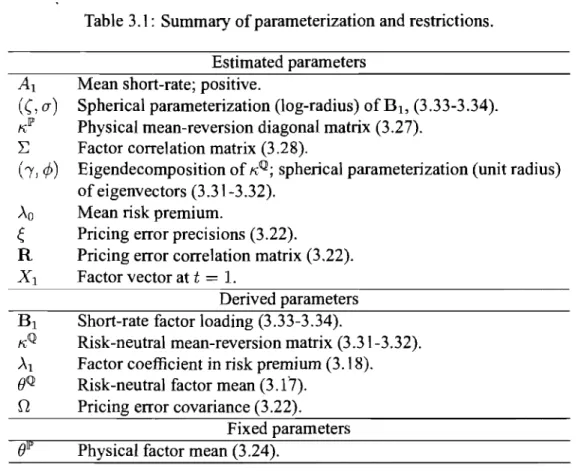
3.5.1 Parameterization. 3.5.2 Prior distributions. 3.6 Posterior simulator . . . . 3.6.1 MCMC algorithm 3.6.2 Mixture sampler . 3.7 Empirical results . . . 3.7.1 Observational errors 3.7.2 Cross-section properties 3.7.3 Time-series properties . 3.8 Conc1uding remarks . . . .

3.9 Appendix A - Prior distribution hyperparameters

. . .

54

55 70 70 74 75 78 80 81 86 89 89 94 101 101 103 104 105 111 112 118 121

3.10 Appendix B - Solution to the pricing difference equation . . . .. 121 3.11 Appendix C - From physical drift to risk-neutral drift in a conditionally

Gaussian model with log-linear SDF . . . . 3.12 Appendix D - VARMA-representation ofyields .. 3.13 Appendix E - Inverse-Gamma-mixture of Gammas 3.14 Appendix G - Principal components . . . .

CHAPITRE 4 : A STATISTICAL ARBITRAGE STRATEGY ON THE

TERM STRUCTURE OF INTEREST RATES.

4.1 Introduction... 4.2 Inference for fixed income portfolios . . 4.2.1 An affine term structure model . 4.2.2 A word on notation . . . . 4.2.3 Misspecification problems 4.3 Bayesian statistical arbitrage . . 4.4 Strategy set . . . .

4.4.1 Delta-hedged portfolios

4.4.2 Mispriced portfolios with execution costs 4.4.3 Investment horizon . . . . .

4.5 Empirical results . . . . 4.5.1 Out of sample performance . . . . 4.6 Appendix A - Prior distributions and hyper-parameters

CHAPITRE 5: CONCLUSION BIBLIOGRAPHIE . . . . 122 123 124 126 127 127 131 131 134 135 137 138 139 142 143 145 145 154 159 163

2.2 Out-of-sample relative performances and weak identification 49 3.1 Summary ofparameterization and restrictions. . 93 3.2 Model notation . . . 105

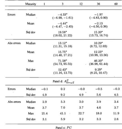
3.3 Pricing errors and covariance modeling 107

3.3 Pricing errors and covariance modeling 108

3.4 Pricing errors and precision modeling 109

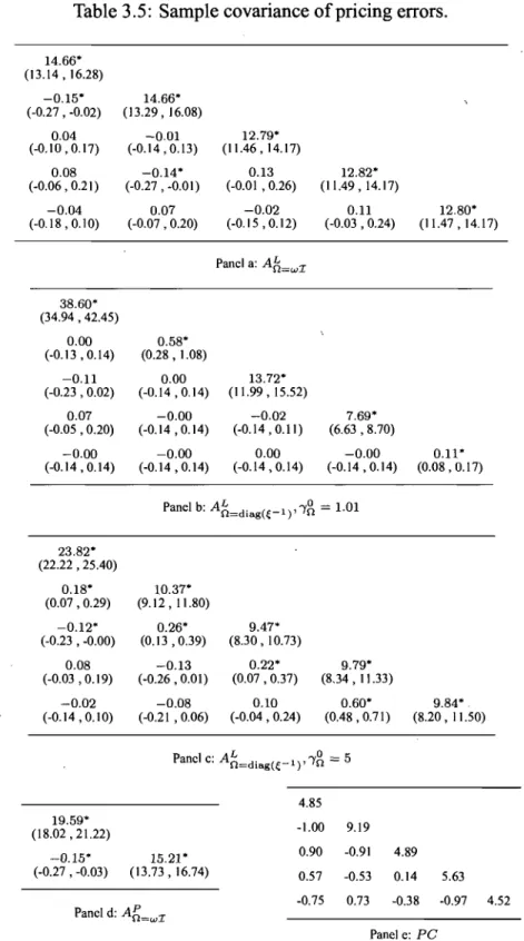
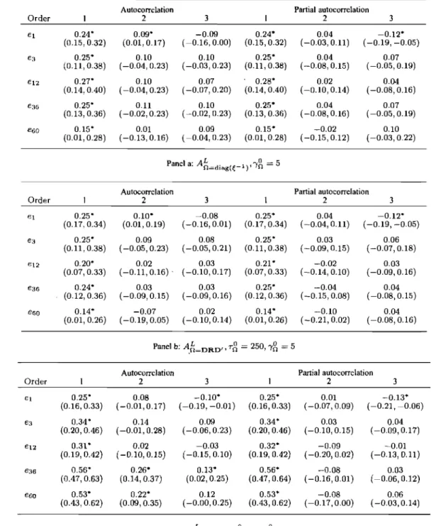
3.5 Sample covariance of pricing errors. . . 113 3.6 Sample auto correlations and partial autocorrelations of pricing errors. 114 3.7 Sample autocorrelations and partial autocorrelations of pricing errors

-Correlation modeling. . . .. 116 3.8 Sample autocorrelations and partial autocorrelations of pricing errors

-Precision modeling. . . . 3.9 Prior distribution parameters for the 3-factor models. 4.1 Summary of indices. . . . .

4.2 Mispriced portfolio statistics 4.3 Optimal portfolio statistics

4.4 Prior distribution hyper-parameter values.

117 121 135 147 150 158

3.1 Sample fonn the pennutation- and reflection-invariant posterior distri-bution of BI. . . . 84 3.2 Sample fonn the nonnalized posterior distribution of BI. . . . . " 85 3.3 Sample fonn the normalized posterior distribution of K~k' k

=

1, ... ,3. 86 4.1 Average gains from mispriced portfolios (t=311 :321). 149 4.2 Optimal portfolio value at risk (h=4). . 152 4.3 Optimal portfolio value at risk (h=10). . . 153

AR ARMA ATSM CIR CRSP DTSM EM EMM GMM IV LSSM MA MAP MCMC ML PC pdf RMSE SDF VAR VARMA Autoregressive Autoregressive-moving -average Affine term structure model Cox -Ingersoll-Ross

Center for Research in Security Priees Dynamic term structure model

Expectation-maximization Efficient method of moments Generalized method of moments Instrumental variables

Linear state-spaee model Moving-average

Maximum a posteriori Monte Carlo Markov chain Maximum likelihood Principal component Probability density function Root mean square error Stochastic discount factor Vector autoregressive

INTRODUCTION

Cette thèse porte sur l'inférence bayésienne pour les modèles affines de la structure à terme des taux d'intérêt (Dai et Singleton, 2002, offrent un survol de la littérature) et de leur utilisation dans un cadre décisionel d'investissement. En particulier, elle met en évidence l'importance de la normalisation de l'espace des paramètres et de la spécification des erreurs observationnelles sur la qualité des prévisions générées par un modèle affine.

Par leur parcimonie et leur solides assises théoriques, les modèles dynamiques de la structure à terme gagnent en popularité dans divers domaines. Outre la construction de portefeuille (Bah, Heidari, et Wu, 2006), on les utilise pour améliorer la prévision de variables macroéconomiques (Ang et Piazzesi, 2003), pour estimer des règles de politique monéraire (Ang, Dong, et Piazzesi, 2007), pour enrichir des modèles néo-keynésiens (Hordahl, Tristani, et Vestin, 2006; Bekaert, Cho, et Moreno, 2006; Dewachter et Lyrio, 2006), et pour estimer des paramètres structuraux, tels des para-mètres de préférence (Garcia et Luger, 2007).

Le premier chapitre de cette thèse, Forecasting with Weakly ldentified Linear Slate-Space Models, considère 1'importance de la normalisation de l'espace des paramètres

sur la qualité des prévisions générées par un espace-état linéraire gaussien. Puisque la vraisemblance de ces modèles est invariante par rapport à certaines transformations des paramètres, l'estimateur du maximum de vraisemblance des paramètres n'est pas unique. On normalise habituellement le modèle en considérant un sous-espace de l'espace des paramètres. Lorsque cette normalisation n'apporte pas l'identification. globale des paramètres, elle est susceptible d'introduire des problèmes d'identification faible se traduisant par un estimateur ponctuel fortement biaisé. Ces problèmes sont bien documentés dans de la littérature sur l'inférence pour les mélanges finis de distributions (Redner et Walker, 1984; Stephens, 2000 ; Frühwirth-Schnatter, 2001 ; Geweke, 2007 ; Hamilton, Waggoner et Zha, 2008), mais leur importance pour les modèles espace-état linéaires n'a pas été étudiée.

Une densité prédictive bayésienne ne repose sur aucun estimateur ponctuel, ce qui lui confère une certaine robustesse à ce problème d'identification faible. Par un exercice de simulation, je compare la performance des prévisions bayésiennes et celles obtenue par la méthode du maximum de vraisemblance, en termes d'erreur quadratique hors échantillon. Je montre que l'avantage des prévisions bayésiennes s'accentue lorsque l'identification des signes des facteurs devient plus faible.

D'un point· de vue méthodologique, je propose un nouvel échantillonneur de Gibbs où les variables dont la loi a posteriori conditionelle n'est pas standard sont tirées

avec les variables latentès en un seul bloc. Je généralise aUSSI l'échantilloneur de permutations proposé par Frühwirth-Schnatter (2001) afin d'explorer efficacement les lobes symétriques de la loi a posteriori invariante des modèles espace-état linéaires.

Le second chapitre, Bayesian Analysis of Affine Term Structure Mo de ls, spécialise

les résultats du premier aux modèles affines de la structure à terme. En particulier, j'utilise une normalisation novatrice du modèle apportant l'identification globale du modèle. De plus, je démontre l'importance de la spécification des erreurs observation-nelles sur l'inférence pour ces modèles. Je montre qu'une spécification courante où la matrice de covariance des erreurs n'est pas de plein rang (Chen et Scott, 1993) peut produire des résidus plus fortement auto-corrélées qu'une spécification de plein rang (Chen et Scott, 1995). Puisque qu'un modèle affine décompose la structure à terme en un certain nombre de facteurs communs et idiosyncrasiques, la spécification de la matrice de covariance des erreurs affecte directement cette décomposition. Par exemple, la modélisation d'erreurs indépendamment et identiquement distribuées impose aux facteurs la lourde tâche de décrire à la fois la dynamique et la covariance contemporaine des taux d'intérêt, que cette 'dernière soit d'origine commune ou idiosyncrasique. En revanche, la modélisation d'erreurs de covariance arbitraire permet d'associer plus étroitement les facteurs aux composantes communes décrivant la dynamique de la structure à terme. Afin d'aller au-delà de ces cas particuliers, je propose nouvelle une loi a priori pour les matrices de covariance. Cette loi permet de spécifier des restrictions

souples sur un continuum entre des erreurs de matrice de covariance arbitraire et des erreurs indépendamment et identiquement distributées.

Il existe peu d'analyses empiriques bayé siennes des modéles affines de la struc-ture à terme. Frühwirth-Schnatter et Geyer (1998), Lamoureux et Witte (2002), Müller et al. (2003), et Sanford et Martin (2005) considèrent des modèles de type CIR. Ang et al. (2007) utilisent échantionneur de Gibbs approximatif où les facteurs latents sont recentrés après chaque itération. Chib et Ergashev (2008) proposent un échantilloneur de Gibbs exact et numériquement efficace. Par contre, au meilleur de ma connaissance, il n'y existe aucune litérature qui tienne compte du problème d'identification faible. Je montre que ce problème empirique est présent dans un jeu de de données couramment utilisées en macro-économie (Ang et Bekaert, 2002; Dai et al., 2005; Ang et Piazzesi, 2003).

Le dernier chapitre, Statistical Arbitrage with Affine Term Structure Models,

uti-lise les résultats des chapitres précédents pour évaluer l'utilité des modèles affines de la structure à terme dans un contexte de construction de stratégie d'arbitrage statistique. L'arbitrage statistique consiste à miser sur les déviations temporaires des valeurs de marchés par rapport à celles données par un modèle. Afin de neutraliser le risque par rapport aux facteurs communs, je construits des portefeuilles dont la valeur est approximativement non corrélée aux facteurs. l'obtiens ainsi un nombre fini de

stratégies, ce qui simplifie la solution numérique du problème d'optimisation. Malgré un problème de spécification évident, la loi prédictive générée par le modèle permet de choisir des portefeuilles générant des gains économiquement significatifs.

FORECASTING WITH WEAKLY IDENTIFIED LINEAR STATE-SPACE MODELS

Abstract

Nonnalizing models in empirical work is sometimes a more difficult task than commonly appreciated. Pennutation invariance and local non-identification cause well-documented difficulties for maximum-likelihood and Bayesian inference in finite mixture distribu-tions. Because these issues arise when sorne parameters are close to being unidentified, they are best described as weak identification (or empirical underidentification) prob-lems. Although similar difficulties arise in linear state-space models, little is known about how they should be addressed. In this paper, 1 show that sorne popular nonnal-izations do not provide global identification and yield parameter point estimators with undesirable finite-sample properties. At the computationallevel, 1 propose a novel pos-terior simulator for Gaussian linear state-space models, which 1 use to illustrate the rela-tionship between forecasting perfonnance and weak identification. In particular, Monte Carlo simulations show that taking into account parameter uncertainty reduces out-of-sample root mean square forecast errors when sorne parameters are weakly identified.

JEL classification: CIl; C5; C52

2.1 Introduction

The likelihood function of many latent-variable models is invariant with respect to certain transfonnations of the parameters. For example, the likelihood function of certain finite mixture distributions is invariant with respect to pennutation of the component distribution indices, leading to an inferential problem known as label

switching in the literature (See Redner and Walker, 1984, for a survey). Consequently,

sorne parameters in latent-variable (or unobserved-component) models are locally unidentified. For mixture distributions, component weights are unidentified in the parameter subspace where component distributions are identical.

Pennutation invariance and local non-identification cause well-documented diffi-culties for likelihood-based inference in finite mixture distributions. Invariance with respect to a set of transfonnations is typically broken through nonnalization: one restricts attention to a particular parameter subspace. For a mixture of two nonnal distributions, one could consider the parameter subspace where the mean of the first distribution is larger than that of the second. It tums out that the choice of nonnalization has critical consequences for parameter point estimators in finite sample. Hamilton, Waggoner, and Zha (2007) [Summary] state that "poor nonnalizations can lead to multimodal distributions, disjoint confidence intervals, and very misleading characteri-zations of the true statistical uncertainty." Because these difficulties arise when sorne parameters are close to being unidentified, they can be described as weak identification

problems in the econometrics literature, or empirical underidentification problems in

the psychometrics literature.

Although weak pennutation and refiection identification cause similar difficulties for inference in linear state-space models (LSSMs), it has received little attention. Jen-nrich (1978) shows that the likelihood function of linear factor models has symmetric lobes because it is invariant with respect to refiections across the axes of the coordinate system, which switch the state variables' sign. Frühwirth-Schnatter and Wagner (2008) stress sorne implications of refiection invariance for univariate linear state-space model selection. With respect to pennutation invariance, Loken (2004) writes "The likelihood and posterior distributions for these models have sorne peculiar properties, and at the very least, researchers employing a Bayesian approach must recognize a multimodality problem in factor models analogous to the label-switching problem in mixture models." To the best of my knowledge, 1 provide the first empirical analysis of the finite-sample

implications of weak permutation and reflection identification for inference in LSSMs. Because these issues are well-known for mixture distributions and these models are simpler than LSSMs, 1 use the former as illustrative examples in this paper.

As the term suggests and is generally understood, a normalization is a restriction of the parameter space (i.e. a parameter subspace) that does not contain any information about the observables or the parameters. From that perspective, normalization is thus in sharp contrast with prior information specification. Therefore, although operationalizing normalization as a restriction of a prior distribution's support is common practice, 1 address normalization and prior specification separately. Doing so isolates the issues pertaining specifically to normalization, which affect both maximum likelihood (ML) and Bayesian inference. Being precise about a third modeling decision, namely parameterization, also proves useful in this paper. Reparameterization consists in defining a one-to-one mapping from one parameter space to another, and often takes the form of a change of coordinate system. Thus, like normalization, parameterization should not contain any information.

1 propose a discussion of normalization which begins with the fundamental, if of-ten side-stepped, question of whèther (or when) normalization is strictly necessary. Because the likelihood function of LSSMs is invariant with respect to a certain set of parameter transformations, standard parameter point estimators are not defined uniquely. Thus, for instance, the maximum-likelihood problem defines a parameter set estimator rather than a point estimator. White normalizing the parameter space in order to obtain well-defined parameter point estimators is common practice, it should be emphasized that normalization is often not strictly necessary. In particular, parameter inference is possible as soon as the parameter set estimator is bounded (Manski, 2003),

which is the case if the likelihood function is invariant with respect to a finite set of parameter transformations.

Because point estimators are simpler from a computational as well as interpreta-tional point of view, they are often preferred to set estimators. in empirical applications. As there are many ways to normalize LSSMs, it is natural to ask how alternative normalizations should be compared. In general, normalizations do not merely ensure that parameter point estimators are well defined, they also have broader implications . for inference. Building on the work of Hamilton, Waggoner, and Zha (2007), 1 argue that normalizations providing global identification are more likely to yield uni modal sampling distributions.

The difficulties associated with reflection local non-identification are closely re-lated to the root-cancelation problem in autoregressive-moving-average (ARMA) models, which were discussed by Box and Jenkins (1976) and are the object ongoing research. Kleibergen and Hoek (2000) propose priors . for a reparameterization of ARMA models in the context of order selection in order to penalize regions of the parameter space where roots are close to canceling out. Stoffer and Wall (1991) study the finite-sample properties of the ML estimator for a LSSM representation of ARMA processes when root-cancelation issues arise. They propose nonparametric Monte Carlo bootstrap standard errors and demonstrate their superiority over the usual asymptotic standard errors.

Point estimators are often less attractive quantities when their sampling distribu-tion are multimodcil. Parameter uncertainty thus plays an important role in such situations. In addition, a symmetric asymptotic approximations of a multimodal

sampling distribution can be umeliable. In contrast, Bayesian inference deals with parameter uncertainty in a consistent manner.

This paper is organized as follows.

ln the first section, 1 describe normalization and weak identification in a general setting. This discussion introduces notation and addresses the questions of whether and when, loosely speaking, normalization is necessary, desirable and feasible. It then tums to comparing alternative normalizations and to practical implementation details.

The second section addresses the invariance of LSSMs with respect to transfor-mations corresponding to linear transfortransfor-mations of the latent state variables. 1 show that a popular normalization described by Harvey (1989) does not provide global identification. Moreover, 1 show that it is observationally restrictive. 1 simplify the analysis of linear transformation invariance by considering elementary transformations: any linear transformation can be decomposed into scaling, rotation, permutation and reflection transformations. Ideal rotation and scale normalizations would preserve permutation and reflection invariance, allowing one to independently specify permu-tation and reflection normalizations. To the best of my knowledge, 1 pro vide the first observationally umestrictive normalization ofLSSMs that provides global identification.

ln the third section, 1 propose permutation- and reflection-invariant prior distri-butions for the parameters of Gaussian LSSMs. Sorne of these priors rely on a reparameterization of the model that is easier to interpret. While normalization and parameterization do not change the informational content of the likelihood function, they might affect the interpretation of the parameters and, consequently, the specification

of prior information. l highlight situations in which one can inadvertently penalize reasonable regions of the parameter space.

In the fourth section, l describe a posterior simulator for G,aussian LSSMs and l explain how to implement reflection and permutation normalizations. 1 first present a Metropolis-within-Gibbs sampler for the parameters whose conditional posterior distributions are not standard. 1 draw these parameters and the latent state variables as a single block. Next, l extend the permutation sampler of Frühwirth-Schnatter (2001) in order to explore the symmetric lobes of reflection- and permutation-invariant posteriors. Although mixing over permutations and reflections is inferentially irrelevant, largue that it helps monitoring the mixing properties of an MCMC simulator in other dimensions.

The fifth section considers the relationship between forecasting performance and weak identification. Because Bayesian predictive densities are reflection- and permutation-invariant, they are not affected by permutation and reflection normaliza-tion. Using simulations, l compare the performance of Bayesian and ML forecasts, on the basis of out-of-sample root mean square errors, and l find that the advantage of taking parameter uncertainty into account increases as reflection identification becomes weaker. l conclude with a research agenda for future research on these matters.

2.2 Weak identification

This section addresses normalization in latent state variable models from a general perspective. l consider likelihood-based inference methods, which rely on a parametric statistical model.

space, :F

{f

(y 1 B) 1 y E

y,

B E

8}

is a set of parametric probability dens ity functions

on

y

and 8 is the parameter set. The likelihood function of the model is the function

l(BI

y)

=

f(yl

B).

The likelihood function of many latent-variable models is invariant with respect to sets of transformations.

Definition 2 Afunction

f :

8 ~ IR is invariant with respect a bijective transformation

T: 8 ~ 8

if

f

(T(B)) =

f

(B)for ail B E 8.

If l(BI y) is invariant with respect to T on 8 for a11 y E

Y

then we say that T(B) and B are observationally equivalent. We will also say that

f

is invariant with respect a set of bjjective transformations T (8) if it is invariant with respect to a11 of its elements. The notation T (8) makes dependence on the set 8 explicit: T (8) is a set of bijections on 8. For example, for 8'

ç

8, T(8') ={T: 8' ~ 8'1 TE T(8)}. 1 will omit this dependence and write T when this causes no confusion. The following examples illustrate this definition.

Example 1 (Normal mean) Consider

y

=

bx

+

e, x r-.J N(O, (j2I) , e r-.J N(O,I),

for (b, (j2) E \li = IR x (0,

00).

The likelihoodfunction,

l(b,

(j21

y) '=

(21fb2~2)T/2

exp { -

2b~(j2Y'Y

} ,

satisfies l (b,

(j21

y)

=

l

(1

Db

l,

(j2 /

D21

y) for any D

=J

0, and it is therefore invariant

TD (8) T_s (8)

TsD

(8) {TD :

8

- t 8ITD(b,a2) = (Db,a2jD2) , D

>

o}

{Ts :

8

- t

81

Ts(b, 0-2)

=

(Sb,a2) ,

ISI

=

1}

{TsD : 8 - t 81 TSD(b, 0-2) = (SDb, 0-2 j D2) , D

> 0,

/S/ = 1} {TSD :

8

- t

81

TSD(b, 0-2) Ts (TD{b,0-2))}

The parameters band 0-2 _{enter the likelihood function as the product b}2 _a2

•

Transforma-tions in T_D correspond to changing the scale of the unobserved factor x and reflect the

fact that (Db? fy~ = b2_0-2 _{for D}

_i=

_o.

_{Transformations in T..c.; correspond to reflections of}

x across the axis x

=

0, which change ifs sign.

Example 2 (Location mixture)

If

the data is a sample from a finite mixture distribu-tion whose K component distribudistribu-tions are from the same parame tric family, then the likelihood has K! symmetric lobes, each lobe corresponding to a permutation of the components' indices. Consider the following mixture of K

with common variance 0-2 and means J.Ll and J.L2

2 normal distributions

Label (or permutation) invariance re/ers to the lilœlihood fonction 's invariance with respect to the re-labeling of the components. Here,

(2.1)

which establishes the invariance to the relabeling (or permuting) of component indices

1 and 2. In matrix notation, a set of invariant transformations is

with 8 =

JR

2

xS

2 X IR, S2 is the simplex ofJR2, J.L

=

[J.Ll J.L21', II

[7r

1

7r1'

and P is a

2.2.1 What is normalization?

In general, transfonnation invariance is addressed by nonnalizing the model. Definition 3 A normalization is a parameter subspace eN

ç

e.

Nonnalizing a model thus defines a new model

(y,

F,

eN).

Example 3 (Normal mean, continued) Some normalizations are

eO"r

{

{;I E

el

0'2 1 },

ebpos _ {{;I E

el

b

>

O},

The normalization

eO"r

defines thefollowing subsets ofinvariant transformations:

{TS :

eO"f

- t

eO"r

1 Ts(b, 0'2) = (Sb, 0'2)

,ISI

1} ,

{TD :

eO"r

- t

eO"r

1 TD(b, 0'2) = (Db, 0'2/ D2) ,D

1} ,

18 (

eO"r)

YD

(eO"î)

Y

SD

(eO"r)

{TSD :

eO"r

- t

eO"r

1 TsD(b, 0'2)

=

(SDb, 0'2/ D2) , D =

1,

ISI

=

1}.

Note that the set YD (

eO"r)

is a singleton, but that there are two transformations in the

sets Ys (

eO"r)

and 18D (

eO"r).

Definition 4 Suppose that a function

f :

e

- t 1R is invariant with respect to a set of

bijective transformations Y(e). A normalization eN

ç

e

breaks the invariance of

f

with respect to Y, which is denoted

where

TI

{T:

e

~

el

T(e) = e}

is a singleton: the identity transformation.

Note that

eN

ç

e

=}

T

(eN)

ç

T

(e).

Breaking invariance with respect to a set of

bijective transfonnations T(e) is thus considering a parameter subspace

eN

ç

e

that is small enough to ensure that the only invariant bijection on that subspace is the identity transfonnation, T(eN

) = {T :

eN

~

eNI

T(e) = el.

Example 4 (Normal mean, continued) Consider the following scaling and reflection transformation sets:

T

s

(e

b) T_s

(eu?)

TD

(e

b)

T

D

(eu?)

T

SD (

eb n eu?)

{Ts :

e

b _~

_ebl

_{Ts(b, 0'2)}

₌

_{(Sb, 0'2) , S}

₌

_I}

₌

_TI,

T

s (e),

T

D (e),

{ TD :

eu?

~

eu?

1 TD(b, 0'2)

=

(Db, 0'2 j D2) ,

D

=

I}

=

TI,

{ TSD :

eb n eu?

~

eb n eu?

1

TSD (b,O'2)

=

(SDb,O'2jD 2), S

=

I,D

=

I}

=

TI.

The normalization

e

b breaks invariance with respect to reflection because T_{s is not a}

bijection on

eb

for S

#-

1. Similarly,

eu?

breaks invariance with respect to scaling

because T D is not a bijection on

eu?

for

D

#-

1. Thus,

e

b

n eu?

breaks invariance with

respect toT_{SD .}

Example 5 (Location mixture, continued) One might contemplate one of the two fol-lowing normalizations:

871"

{e

E

817r

> 0.5}

81l

_{e

E

81

ILl

>

IL2}'

Each normalization would break permutation invariance as T

(871")

=

T (81l )

=

TI.

One could consider nonnalizations of arbitrary fonn, but 1 restrict the following discus-sion to intersections of half spaces and hyper-planes,

l J

8N =

n

{e

E

81

g~e >

O}

n

n

{e

E

81 hje

=

O},

i=l j=l

for sorne confonnable real vectors gl, ... , gI, hl, ... , hJ . For exarnple, one would break

invariance with respect to a set of

(1+

1)! invariant transfonnations with a nonnalization consisting in the intersection of 1 half spaces. In contrast, the intersection of J hyper-planes would break invariance with respect to a set of invariant transfonnations that is equinurnerous to ~J (i.e a set T that has the same cardinality as ~J).

Example 6 (Normal mean, continued) There are 2! transformations in T_s(8) and the half space

{e

E

81

b

>

O}

breaks invariance with respect to reflections. The set TD

(8)

is equinumerous to ~ (e.g. the naturallogarithm is a bijectionfrom

(0,00)

to~) and the

line

{e

E

81

(72

=

1} breaks scale invariance.

Note that considering intersections ofhalfspaces and hyper-planes is not as restrictive as it rnight seern. In particular, one can consider half spaces and hyper-planes in any space that is homeornorphic to 8. In section 2.3, for example, 1 repararneterize sorne vectors in polar coordinates and 1 nonnalize in the space of angles and lengths.

2.2.2 Is normalization necessary?

When the like1ihood function of a latent-variable model is invariant with respect to a certain set of parameter transfonnations, the rnaximurn-like1ihood problem defines a

parame ter set estirnator rather than a point estirnator,

{ 0 E

e

1 0 = arg max l (0'1

y)} .

9'E8

Example 7 (Location mixture, continued) Permutation invariance implies that the

likelihood function admits two equivalent global maxima, sitting at the summit sym-metric lobes:

if

(p,

ft,

êJ)

is a global maximum, so is

(pp, pft,

êJ),

for P =

[~

6].

While norma1izing the pararneter space in order to obtain well-defined ML pararneter point estirnators is cornrnon practice, it should be ernphasized that normalization is of-ten not strictly necessary. In particular, pararneter inference is feasible as soon as the pararneter set estirnator is bounded (See Manski (2003) for a textbook treatrnent, and Chernozhukov et al. (2007) and Galichon and Henry (2009)). In terms of conditions on transformation sets, a sufficient condition is therefore that the set can be pararneterized and that this pararneter is bounded.

Definition 5 A set of transformations

is bounded if

:r

is a bounded set.

Example 8 (Normal mean, continued) The ML parameter set estimator of 0 on

eO"?

is bounded as

TsD (

eO"?)

is bounded.

From a Bayesian perspective, as long as priors are proper, posteriors are proper and the model is "identified" in that specifie sense, but Bayesian inference is not immune to invariance issues. Although it is cornrnon practice to operationalize normalization through a truncation of the prior distribution, considering normalization and prior specification independently makes exposition clearer. 1 therefore consider priors such that f(O)

>

0 for all 0 E

e

in this paper.

1 will argue in Section 2.4 that it is conceptually inconsistent to express prior be-liefs over the relative plausibility of observationally equivalent parameter values. In other words, if the likelihood function is invariant with respect to a given transformation set, prior distributions should also be invariant with respect to that set.

Example 9 (Location mixture, continued) The proper prior distribution f (fJ,) N(fJ,1

0,1)

is invariant with respect to Tp (8).

This raises the question of whether there always exists a proper prior on 8 that is in-variant with respect to any given set of transformations T (8). This is obviously not the case. It is possible to specify a proper prior that is uninformative about (uniform over) observationally equivalent parameter values if and only if the transformation set T is bounded.

Example 10 (Normal mean, continued) f(yl b,

(72)

is invariant with respect to 78(8)

and TD(8). Finding a proper joint prior distribution that is invariant with respect to

78(8) _{is straightforward. For example, ajoint prior is invariant with respect to Ts}(8)

as soon as its marginal prior f(b) is symmetric and centered on zero. In contrast, there exists no properjoint prior f(b,

(72)

such that f(b,

(72)

= f(ab, (72/a21 a) for ail a E

A

=

(0,00) as this wou Id require that the prior be constant over unbounded sets.

Thus, Bayesian and ML inference for set estimators is possible when T is bounded. When T is not bounded, it is sometimes possible to write transformations in T as com-positions of other transformations and identify a bounded subset of transformations.

Example 11 (Normal mean, continued) TSD (8) is unbounded, but TSD(b, (72)

Ts(TD(b,

(72))

_{and Ts (8) is bounded Therefore, one needs not break invariance with}

respect to riflections in order to make inference for (b,

(72).

For example, parameter set

estimators are well-defined under 8cr

_î

This example illustrates that one can sometimes write an unbounded transformation set as the composition of smaller bounded and unbounded subsets. Breaking invariance with respect to the unbounded subset is sufficient for set estimators to be bounded.

2.2.3 What are the costs and benefits of normalization?

Because point estimators are simpler from a interpretational as well as computa-tional point of view, they are often preferred to set estimators in empirical applications. Indeed, ML inference often calls for simulations methods (For example, Jacquier et al. (2007) show how a simple modification of the Bayesian MC MC algorithm produces the ML point estimate and its asymptotic variance covariance matrix.) and non connected confidence sets constitute a challenge to communication empirical results.

ln the Bayesian framework, if prior distributions and the likelihood function are invariant with respect to a set of transformations T, then so are posterior distributions. Invariant proper prior and posterior distributions are perfectly valid characterization of uncertainty. In cases where

T

is finite (but not a singleton), sorne posterior distributions are multimodal and thus cause interpretational difficulties. For example, if the bimodal posteriors of J1.1 and J1.2 in (3.5) are symmetric with respect to zero, the posterior means of these parameters are both equal to zero, IE.[J1.1Iy]

=

E[J1.2IY]

=

0 which is not particularly informative about the mixture components.

The model should therefore be normalized if the investigator uses mixtures or LSSMs as classification tools where the interpretation of the components or state variables is of interestl

. When the parameters are not of direct interest however, such as when one uses latent-variable models as flexible parameterizations of the observables's

distribution, transfonnation invariance introduces no interpretational difficulty and nonnalization, beyond what is required in order to obtain weIl defined set estimators, is unnecessary.

In general, a multimodal posterior distribution also constitutes a computation challenge for a basic posterior simulator, but posteriors in latent-variable are no general multi-modal distributions: they are symmetric. Symmetry has two important implications. First, because any lobe contains aIl relevant infonnation about the parameters, one can consider any single one of them. Second, because aIl lobes are equivalent, the mixing properties of a posterior simulator over pennutations are irrelevant (Geweke, 2007).

2.2.4 Are the potential benefits of normalization always achievable?

In sorne cases, nonnalization can fail to provide its expected benefits and ML parameter point estimators can have multimodal sampling distributions, which causes concems equivalent to those we have with set estimators. For example, multimodality can imply disjoint confidence intervals. Similarly, parameter posterior distributions can be multimodal. In such situations, interpretational benefits are lost. In addition, symmetric asymptotic approximation are unreliable and one must thus obtain sampling distributions by simulation methods.

These problems anse when sorne elements of () are weakly identified. Except in the context of instrumental variables (IV) and the generalized method of moments (GMM), weak identification has not been defined precisely. Dufour and Hsiao (2008) write: "More generaIly, any situation where a parameter may be difficult to detennine because we are close to a case where a parameter ceases to be identifiable may be called weak identification." Many common situations fit this description. For example,

multicollinearity issues arise in linear regression models when the sample covariance matrix of the regressors is "close" to being singular. If one restricts attention to ML inference, weak identification problems occur when the Fisher information matrix is close to being singular at the pseudo-true parameter values. Thus, weak identification is a joint property ofboth the model

(y,

F,

eN)

and the data y, as the term "empirical underidentification" used in psychometries emphasizes. In this paper, l say that a parametric model is weakly identified if

ê

(eN)

is close to

el,

where

el

ç

e

is the singularity parameter subspace where the Fisher information matrix is singular. Example 12 (Location mixture, continued) The information matrix is singular on

{e

E el

/-LI = /-L2}

c

e'll",

where the probability 7r is unidentified. Thus we say that the

model is weakly identified

if

the pseudo-true parameters /-LI and /-L2 are too close to each

other. ln such situations, the lobes of the likelihood function are not weil separated and they are not symmetric with respect to their respective mode. A symmetric normal

ap-proximation of the ML estimators 's sampling distribution is thus unlikely to be accurate.

lndeed, Dick and Bowden (1973) compare a Monte Carlo approximation of the

param-eter sampling variances to their asymptotic counterparts, which are approximated by a

power series expansion of the information matrix developed by Hill (1963). They report

that [SummaryJ "the sample variance of the estimates can be as much as three limes greater than the estimated asymptotic variances ".

Weak identification has severe consequences for ML inference, which Dufour and Hsiao (2008) summarize thus:

" ... standard asymptotic distributional may remain valid, but they constitute very bad approximations to what happens in finite samples:

.1. standard consistent estimators of structural parameters can be heavily biased and follow distributions whose form is far from the limiting

Gaussian distribution, such as bimodal distributions, even with fairly large samples (Nelson and Startz, 1990; Hiller, 1990; Buse, 1992); 2. standard tests and confidence sets, such as Wald-type procedures based

on estimated standard errors, become highly unreliable or completely invalid (Dufour, 1997)"

How close is too close? As weak identification is a finite-sample concern, one might be tempted to believing it is only a small-sample concern. Even for fairly large sample sizes, however, the asymptotic approximation of the ML estimator's sampling distri-bution may be unreliable. Bound et al. (1995) present an IV situation in which weak identification difficulties persist even with 329000 observations. Intuitively, if the instru-ments were uncorrelated with the regressors in population, increasing the sample size would be futile. In practice however, the statistician never knows the pseudo-true param-eter values and he should favor inferential methods that are robust to weak identification.

ML parameter point estimators are less attractive quantities when their sampling distribution are multimodal. For the same reasons that normalizations do not guarantee unimodal ML estimator sampling distributions, they do not guarantee unimodal posterior distributions (See Stephens (2000) for a discussion). Parameter uncertainty plays an important role is such situations. Bayesian inference deals with parameter uncertainty in a consistent manner. While standard ML forecasts rely on parameter point estimates, Bayesian forecasts average over the parameter posterior distribution. When weak identification issues arise and point estimators become unreliable, the simulations results presented in this paper reveal that the richer information content of posterior distributions yields better out of sample forecasts. Bayesian analysis has proved a useful framework for other weak identification problems. For example, Leamer (1973) provides an illuminating interpretation of multicollinearity. In this paper, I build on the

fact that global identification is unnecessary for forecasting pUI-poses. Whether sorne parameters are subject to weak identification problems is therefore irrelevant.

2.2.5 How best to normalize?

Because there are many ways to normalize a model, it is natural to ask how alternatives should be compared. This paper proposes three criteria for choosing normalizations.

A first natural criterion is that a normalization should be observationally unrestrictive.

Definition 6 Suppose l (() 1 y) is the likelihood function of a parametric statistica/ mode/

(y,.1",

e).

A normalization

eN

ç

e

is observationally un restrictive

if

there exists a

transformationg:

e -

eN

suchthatl(g(B)/y) = l(B/y)forally E

y.

Anormalization

is observationally restrictive otherwise.

The two other criteria pertain to the shape of point estimator sampling or parameter posterior distributions. Obviously, multimodality issues will arise more often if the normalization is disconnected. A second criteria is thus that the normalization should be connected2

• Note that intersections ofhalf spaces and hyper-plans are connected spaces. AIso, continuous bijections preserve connectedness (Royden, 1988).

Global identification does not only ensure ML estimator's uniqueness, it also affects its sampling distribution. If global identification is achieved through normalization, then normalization has implications for estimator sampling and parameter posterior distributions. Hiller (1990) shows how normalization in structural equations models af-fects the finite-sample distribution of ordinary least squares and two-stage least squares

2 A space eN is said to be connected if there do not exist two nonempty disjoint open sets 01 and O2

estimators. Unfortunately, as Hamilton, Waggoner, and Zha (2007) note, "the fact that nonnalization can materially affect the conclusions one draws from likelihood-based methods is not widely recognized."

Hamilton, Waggoner, and Zha (2007) propose an identification principle as a general guideline for the choice of nonnalizations, advising that one should [p. 225] "make sure that the model is locally identified at all interior points". More generally, weak identification difficulties are amplified when the mode1 is not globally identified. Global identification thus defines a third preorder on nonnalizations: Nonnalizations providing global identification are more likely to produce unimodal sampling distributions and thus alleviate weak identification issues.

ln this paper, 1 use the following definition, which captures the three criteria de-scribed above:

Definition 7 A normalization

eN

ç

e

satisfies the identification principle

if

il .

a) is observationally unrestrictive;

b) is connected;

c)

provides global identification.

The following examples illustrate how disconnectedness and local non-identification can produce multimodal estimator sampling distributions.

Example 13 (Normal mean, continued) The disconnected normalization ebdiSC

{() E

el

b E [-1,0) U (1,00)} provides global identification and is observationally

un-restrictive. However, it would pro duce a bimodal sampling distribution for

b

if

the true

Example 14 (Location mixture, continued) The sampling distributions of the ML

es-timator of JLI and

JL2

can be multimodal under 81f

• Intuitively, this normalization would

perform poorly

if

the data came from a mixture distribution with 7r 0.5 because

com-ponent densifies would be equiprobable. The identification principle rules out 81f

be-cause the Fisher information matrix is singular on {O E

81

JLI JL2,7r 0.5} C 81f

• In

contrast, the model is globally identified on 8M•

In the latter example, the identification princip le yields a unique normalization, under which the ML estimator has a unimodal sampling distribution for any () E 8M• In slightly more general models, the identification principle is less straightforward to· ap-_,. ply, as it may yield uncountably many normalizations. The practical guidance that the identification principle offers is thus incomplete. Moreover, there is no guarantee that any particular normalization ensures that the ML estimator has a unimodal sampling distribution.

Example 15 Consider the location-and-scale mixture of normal distributions

f(YtIJLbJL2,7r,O'i,a~)

= 7r4>(YtIJLl:ai)

+

(1

~ 7r)4>(YtIJL2,0'~)'

The set where the iriformation matrix is singular is not a line but a point,

The identification principle still rules out restrictions based on 7r, but the singularity subspace no longer separates the parameter space into two symmetric half-spaces.

Nor-malizations

8

M _and

both satisfY the identification principle, but neither ensures that ail sampling

and al

>

a2. Under

8/1-,

the ML estimator of al and a2 will have bimodal sampling distributions for sufficiently large samples (Geweke, 2007).

It cannot be overemphasized that the identification principle does not "solve" the weak identification problem. While it usefully d~fines a preorder on normalizations, it falls short of recommending a unique optimal normalization. Moreover, the identification principle does not ensure that standard asymptotics provide reliable approximations of ML estimator sampling distributions, and one should resort to simulation methods to accurately characterize the true statistical uncertainty of ML estimators.

Therefore, although unimodal sampling or posterior distribution may be desir-able, they cannot be guaranteed. One can try a number of normalizations satisfying the identification princip le and hope to find one that yields estimators with acceptable finite-sample properties. For ML inference, comparing competing normalizations can be impractical. For each, one should obtain sampling distributions by simulation methods. Because the ML estimator does not have a closed-form solution, this involves substantial computational costs.

Stephens (1997) shows that normalizations can equivalently be applied within a posterior sampler or as a post-simulation step on the output from an un-normalized sampler. Using the latter implementation, one can compare competing normalizations with negligible computational cost. Indeed, because normalizations truncate poste-riors but do not change their informational content, they can be chosen a posteriori (Frühwirth-Schnatter, 2001). However, this exercise can be difficult in high-dimensional models.

2.2.6 Summary

Inference in latent variable models is possible as soon as the set of transformations with respect to which the likelihood function is invariant, is finite. One then has pa-rameter set estimators. One can normalize further in order to obtain papa-rameter point estimators. This might ease interpretation and computation, but can make inference sen-sitive to weak identification issues. In particular, parameter point estimates are unreliable quantities if the estimator's sampling distribution is multimodal, and parameter uncer-tainty should be taken into account. AIso, exact sampling distributions are required in order to correctly describe statistical uncertainty. When parameter point estimates are of direct interest, connected normalizations that provide global parameter identification are more likely to produce unimodal sampling or posterior distributions. Comparing many such normalizations might prove useful. This is computational trivial in the Bayesian framework, but often impractical in the ML framework as estimators are not available in c10sed form.

2.3 Normalization of LSSMs

In the notation of Hamilton (1994), let Yt be a N-dimensional vector of observables at time

t,

~t an latent (or unobserved) K -dimensional vector of latent state variables, and Xt a l-dimensional vector of observed exogenous variables. A Markovian Gaussian linear state-space model is defined by the system of equations

~t+l Yt F~t

+

Vtl B

+

A'Xt

+

H'çt

+

Wtl

(2.2) (2.3)

where Vt and Wt are Gaussian white noises with covariance matrices Q and R,

respectively3. Equation (2.2) is referred to as the state equation and equation (2.3) as

the observation equation. State variables are also known as factors and H as the matrix

offactor loadings. For expositional c1arity l consider only the case A = 0 and N ~ K,

but this is not a substantive restriction.

The likelihood function is invariant with respect to invertible linear transformations of the latent variables; for any invertible M,

l(B, M,-lH, R, MFM-1

, MQM', M6IYt) l(B, H, R, F, Q, 6IYt). (2.4)

Thus, the system (2.2-2.3) can be written as F çt

+

Vt, Yt B

+

A'Xt

+

fI'~t

+

Wt, where

fI

= M,-lH,

F

= MFM-1_,

Q

_{= MQM', ~ = Mç and}

v

_{= Mv.} 2.3.1 Primitive transformations (2.5) (2.6)

In order to highlight the weak identification issues, it is useful to consider primitive transformations M = {D, 0, P, S}, where

• D is a diagonal, positive-definite scaling matrix; • 0 is a rotation matrix;

• P is a permutation matrix;

• S is a diagonal reflection matrix with elements equal to 1 or -l.

Let TD , T

o ,

Tp and

Ys

denote these four sets of primitive transformations. Permutation and reflection matrices are orthogonal matrices, i.e. P'P

=

S'S

=

I; rotation matrices are special orthogonal matrices, i.e.

0'0

=

I and

101

=

1. Any linear transformation can be decomposed into these primitive transformations in order to help c1arifying invariance issues.

Note that the sets

Ys,

Tp and T

_o

are bounded. Indeed,

Ys

contains 2K transfor-mations, Tp contains K! transformations, and T

_o

can be parameterized by K(K -1)/2 angles. This means that breaking scale invariance is sufficient in order to make inference in LSSMs.

As permutation invariance in mixture distributions, permutation and reflection invari-ance makes the likelihood function of LSSMs multimodal and local non-identification introduces weak identification concems. Intuitively, permutations are weakly identified when factors are too similar, and reflections are weakly identified when factor loadings are too smal1.

A much-cited reference on LSSM normalization is Harvey (1989). He writes (for the special case F = T) (p.451):

"In order for the model to be identifiable, restrictions must be placed on

[Q]

and

[H].

In c1assical factor analysis, the covariance matrix of the common factors is taken to be an identity matrix. However, this is not sufficient to make the model identifiable since if

[M]

is an orthogonal matrix, [(2.5-2.6)] still satisfies aU the restrictions of the original model because [Var(Mvt) = MM' =

11.

Sorne restrictions are needed on [M], and one way ofimposing them is to require that the ij-th e1ement of

[M],

[Mij ], be zero for j

>

i,

i = 1, ... , K - 1. Altematively,

[Q]

can be set equal to a diagonal matrix while [M_{ii ]}

=

0 for j

>

i and

[Mii]

=

1 for i

=

1, ... ,K."

The proposed normalization are

e

QI

n

_{e Hlt and eQdiag}

n

e

_{Hlut , where}

eQdiag _ {() E

el

Q is diagonal} ;

e

QI

{() E

el

Q

=

1};

e

Hlt _{_ {() E}

_el

_{H has a lower triangular KxK block};}

e

Hlut

{() E

el

H has a lower unitriangular K xK block} .

A unitriangular matrix is triangular and has ones on the main diagonal. It is straight-forward to show that these normalizations break invariance with respect to scaling, rotation, reflection and permutation. However, they do not provide global parameter identification. Moreover, these normalizations are observationally restrictive.

Both of Harvey's normalizations are observationally restrictive because they in-volve K 2 _{parameter restrictions while breaking scale invariance requires K restrictions}

and breaking rotation invariance requires K(K - 1) /2 restrictions. Thus, K(K - 1) /2

additional parameter restrictions reduce the model's flexibility. 1 will present several normalizations in this section, but consider a simple one here in order to illustrate how one can normalize scales and rotations with K(K

+

1) /2 restrictions. The central issue is that identity matrices are diagonal matrices with diagonal elements aIl set to l, which implies that MIM' = l if M is an orthogonal matrix. In contrast, consider diagonal matrices with diagonal elements set to distinct values, say Qkk

=

k for k

=

1, ... , K.

Because MQM' =1= Q when M is orthogonal, these K(K

+

1) /2 restrictions break rotation and scale invariance.

identification, we first need to find a parameter subspace where sorne parameters are locally unidentified. Then, we need to show that the intersection of this subspace and the interior of the normalization is not empty. For example, consider the parameter subspace where the first column of H is a vector of ones and its other elements are all zeros. This subspace in strictly contained in both e Hlt and eH/ut. Permutation

invariance is broken by e Hlt or eH/ut because permuting the rows of a triangular matrix

does not yield, in general, a triangular matrix. Thus, row permutation is not a bijective transformation on the space of triangular matrices. However, row permutation is a bijective transformation on the region described above: the fust column of PH would be a vector of ones and its other elements would be aIl zeros. Thus e Hlt and eH/ut do

not provide global identification.

1 proceed to propose connected, observationally unrestrictive normalizations providing global identification. To the best of my knowledge, these are the first normalizations of LSSMs satisfying the identification princip le. Although the concepts are easily extendable to other distributions, 1 present normalizations for Gaussian LSSMs for expositional c1arity.

2.3.2 Breaking rotation invariance

The likelihood function of LSSMs is invariant to geometric rotations of state variables in Euc1idean space: for given parameter values Q, H and F, any rotation matrix 0 defines observationally equivalent parameter values

Q

=

OQO',

fI

=

O,-lH and

F

= OFO-1

. Any K -dimensional rotation matrix can be parameterized by K(~-l) angles.