Shared Control Based on an Ecological Feedforward and a Driver Model Based Feedback

HAL Id: hal-02110825

https://hal.archives-ouvertes.fr/hal-02110825

Submitted on 25 Apr 2019

HAL is a multi-disciplinary open access

archive for the deposit and dissemination of

sci-entific research documents, whether they are

pub-lished or not. The documents may come from

teaching and research institutions in France or

abroad, or from public or private research centers.

L’archive ouverte pluridisciplinaire HAL, est

destinée au dépôt et à la diffusion de documents

scientifiques de niveau recherche, publiés ou non,

émanant des établissements d’enseignement et de

recherche français ou étrangers, des laboratoires

publics ou privés.

Shared Control Based on an Ecological Feedforward and

a Driver Model Based Feedback

Béatrice Pano, Yishen Zhao, Philippe Chevrel, Fabien Claveau, Franck Mars

To cite this version:

Béatrice Pano, Yishen Zhao, Philippe Chevrel, Fabien Claveau, Franck Mars.

Shared Control

Based on an Ecological Feedforward and a Driver Model Based Feedback.

9th IFAC

Interna-tional Symposium on Advances in Automotive Control, Jun 2019, Orléans, France. pp.385-392,

�10.1016/j.ifacol.2019.09.062�. �hal-02110825�

Model Based Feedback

Béatrice Pano*. Yishen Zhao*. Philippe Chevrel*. Fabien Claveau*. Franck Mars **



*IMT Atlantique, LS2N UMR CNRS 6004 (Laboratoire des Sciences du Numérique de Nantes), 44307 Nantes, France

(e-mails : firstname.lastname@ls2n.fr)

** CNRS & Centrale Nantes, LS2N UMR CNRS 6004 (Laboratoire des Sciences du Numérique de Nantes), 44321

Nantes, France (e-mail : firstname.lastname@ls2n.fr)

Abstract: Haptic shared control is a consistent way to design an assistance for the lateral control of a vehicle. The most important problem raised by haptic shared control is to minimize useless conflicts between the driver and the assistance. To deal with, this paper proceeds in two stages. The first is concerned with feedforward synthesis in a new way, by identifying mainly the geometric part of driving from real driver data. The torque to apply to the steering wheel and more generally the reference trajectory is thus obtained from a second order model fed by the road curvature. Then, the feedback is designed based on a driver-vehicle-road model, using a mixed 𝐻2/𝐻∞ control synthesis involving both lane following

performance and sharing capabilities indicators. Finally, the shared control strategy is simulated on Matlab/Simulink using a vehicle-road model. The results obtained show good features both in terms of lane following and sharing performances. This control strategy seems then to be an interesting candidate for haptic shared control.

Keywords: Identification for control, Shared control, cooperation and degree of automation, Robust control, Vehicle dynamic systems

1. INTRODUCTION

Haptic shared control in the context of lateral control of a vehicle is a solution which allows to involve both the controller and the driver in the steering task. It is investigated in the literature as it improves the lane following performance (Benloucif et al., 2017; Griffiths and Gillespie, 2004; Saleh et al., 2013). Moreover, it can increase the security on the road which is a big challenge in today’s world; for example, by preventing the driver to come out of the road when doing a second task (Blaschke et al., 2009).

By using a haptic interface for shared control, the communication between the assistance and the driver is improved. The driver can know the command applied by the assistance through the steering wheel. But this communication have to be intuitive for the driver in order to minimize conflicts between the assistance and the driver (Abbink et al., 2018; Mugge et al., 2016). Then, using a driver model to synthetize the assistance make its actions more understandable for the driver and decreases the control effort applied by the driver (Abbink et al., 2012).

Efficient solutions for haptic shared control were proposed earlier using a cybernetic driver model (Saleh et al., 2013; Sentouh et al., 2009) to predict its short term intention and so favouring cooperation over contradiction. The driver model was identified successfully from real drivers (Saleh et al., 2011) on the LS2N driving simulator and from real car experiments (Hermannstädter and Yang, 2013). Here, the

authors propose to adopt another strategy, making a clear separation between feedforward and feedback actions, to facilitate possible interaction with the tactical level of autonomous cars. Moreover, the feedforward proposed doesn’t require infinite dimension FIR model implementation (Saleh et al., 2013).

Explicit separation between feedforward and feedback was sometimes considered for lateral control of autonomous vehicles (Attia et al., 2012; Kapania and Gerdes, 2015; Kuwata et al., 2008), but in a different context, not considering torque command and haptic interactions. The aim in this paper is to take the driver into account in both parts. The feedforward relies on a model identifying mainly the geometric part of driving in order to supply a reference trajectory. The feedback is based on a 𝐻2/𝐻∞ output feedback taking benefits of a

driver-vehicle-road dynamic model, by optimizing some criteria linked with the lane following and sharing performances and with robustness.

This paper is organised as follows: section 2 shows the global architecture model used for the haptic shared control strategy. Section 3 presents the way of using identification theory for the feedforward part synthesis of the e-copilot, aiming for an ecological lateral control. Section 4 presents the 𝐻2/𝐻∞

control synthesis proposed for the feedback part, from the driver-vehicle-road model together including the feedforward action. Section 5 presents the simulation conditions used to assess the control strategy and the results obtained. Finally, the conclusion take place in section 6.

2. SHARED CONTROL STRATEGY

2.1 Architecture

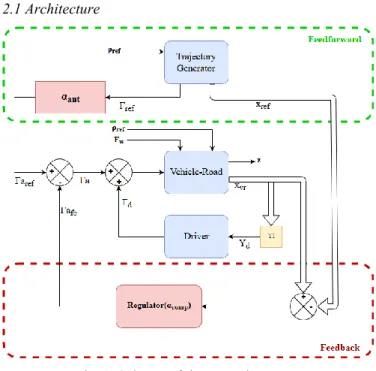
Fig. 1. Scheme of the control strategy

The shared control strategy proposed here is split in two parts (see Fig. 1.). First, a feedforward (green dotted rectangle), which consists in a global identified model of a driver model in interaction with the vehicle-road model (see section 3). This model allows to obtain a reference trajectory constituted by the torque command reference and the state reference for the feedback part. Secondly, a 𝐻2/𝐻∞ feedback part (red dotted

rectangle) is designed to make the vehicle following the reference trajectory in spite of disturbances, while guarantying good sharing properties (for acceptability purposes). The design methodology associated to this part is detailed in section 4.

The two parts, feedforward and feedback are designed sequentially. The level of sharing is controlled at two different places materialised by the two parameters 𝛼𝑎𝑛𝑡 and 𝛼𝑐𝑜𝑚𝑝.

2.2 Systems modelling

The useful model for design and simulation, and the associated signals that will be manipulated all along this paper can be defined as follows; a vehicle-road model described in (Saleh et al., 2013) which represents the dynamics of the vehicle and the position of the vehicle on the road can be written as:

𝑥̇𝑣𝑟 = 𝐴𝑣𝑟𝑥𝑣𝑟+ 𝐵1𝑣𝑟(Γ𝑎+ Γ𝑑) + 𝐵2𝑣𝑟𝜌𝑟𝑒𝑓+ 𝐵3𝑣𝑟𝐹𝑤 (1)

With 𝑥𝑣𝑟 = [𝛽 𝑟 𝜓𝐿 𝑦𝐿 𝛿𝑑 𝛿𝑑̇ ]𝑇 the vehicle-road

state where 𝛽 is the slip angle, 𝑟 is the yaw rate, 𝜓𝐿 is the

heading error angle, 𝑦𝐿 is the lateral error between the vehicle

and the road centre at the look-ahead distance 𝑙𝑠 and 𝛿𝑑 is the

steering wheel angle. Γ𝑎 and Γ𝑑 are respectively the assistance

and the driver torque applied on the steering wheel, 𝜌𝑟𝑒𝑓 is the

road curvature and 𝐹𝑤 is the side wind resultant applied on the

gravity centre of the vehicle. Matrices 𝐴𝑣𝑟, 𝐵1𝑣𝑟, 𝐵2𝑣𝑟 and

𝐵3𝑣𝑟 can be found in (Saleh, 2012b; Saleh et al., 2013).

The driver model explicitly represented in Fig. 1. (blue box) is a cybernetic driver model (3rd _{order model) designed and}

identified according to the approach proposed in (Mars and Chevrel, 2017; Saleh et al., 2011). The procedure will not be recalled here, but the main point is that coherently with a real driver, the model’s input is made of the near and far visual points 𝜃𝑛𝑒𝑎𝑟, 𝜃𝑓𝑎𝑟, the self-aligning torque Γ𝑠, and the steering

wheel angle 𝛿𝑑 and the model’s output is the torque applied by

the driver to the steering wheel Γ𝑑.

𝑥̇𝑑= 𝐴𝑑𝑥𝑑+ 𝐵𝑑[𝜃𝑓𝑎𝑟 𝜃𝑛𝑒𝑎𝑟 𝛿𝑑 Γ𝑠]𝑇 (2)

Γ𝑑= 𝐶𝑑𝑥𝑑

Then, the dynamic model is identified from experimental data either from a driving simulator in (Ameyoe et al., 2015; Saleh et al., 2011) or a real car in (Hermannstädter and Yang, 2013). In this study, this model is supposed to be known and will be used for the feedback part of the haptic shared control. Notice that the yellow case T1 in Fig. 1. represents the calculation done from the vehicle-road state 𝑥𝑣𝑟 to obtain the driver model

inputs 𝑌𝑑= [𝜃𝑓𝑎𝑟 𝜃𝑛𝑒𝑎𝑟 𝛿𝑑 Γ𝑠]𝑇.

The next two sections give details on the design methodology for the feedforward and feedback parts, both taking into consideration the driver behaviour, but through two different driver model identifications.

3. FEEDFORWARD DESIGN: GEOMETRIC DRIVING IDENTIFICATION

3.1 Trajectory generator

The reference trajectory involved in the feedforward part in Fig. 1. can be detailed as in Fig. 2.

Fig. 2. Trajectory generator

The reference trajectory is composed of the torque Γ𝑟𝑒𝑓 and the

vehicle-road state 𝑥𝑟𝑒𝑓 , these signals are assumed to be close

to those which were found if the driver would have driven the vehicle alone. This can improve considerably the results in terms of sharing performance by decreasing conflicts between the driver and the assistance. That is why the level of sharing of the feedforward part is applied on the reference command torque as : Γ𝑎𝑟𝑒𝑓 = 𝛼𝑎𝑛𝑡Γ𝑟𝑒𝑓.

3.2 Trajectory generator design methodology

Among classical solutions, one may quote (Rajamani, 2012) which manipulates the bicycle model to find relationship between the road curvature assumed to be constant and a consistent reference trajectory; that is to say a constant steering wheel angle, yaw rate and steering angle, a zero lateral error, and what they have called the desired heading error angle. Note that this solution can be limiting (though very useful and used), both by its restrictive hypothesis (constant curvature), and by the fact that the output considered is the steering wheel angle and not the torque. What is proposed is to make use of experimental data from the driver to identify the geometric part of driving, to obtain Γ𝑟𝑒𝑓 and 𝛿𝑑_𝑟𝑒𝑓 , associated to the

vehicle-road model, leading to (𝛽𝑟𝑒𝑓, 𝑟𝑟𝑒𝑓, 𝜓_{𝐿 𝑟𝑒𝑓}, 𝑦_{𝐿 𝑟𝑒𝑓}, 𝛿̇_{𝑑𝑟𝑒𝑓}). More

precisely, the model to be identified is the one making possible to predict part of driving that can be explained directly from the road curvature. So it doesn’t constitute a driver model as the one considered in (2), but rather its projection for feedforward control use, hoping the latter is more ecological than classical solution.

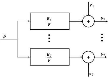
The assumption made here is that, when driver is steering the vehicle following a curve, there exists a reference torque and angle to be applied on the steering wheel if the road curvature is known. The driver will actually act back and forth on the steering wheel to change the torque and angle, to stay around the reference values sought on the basis of geometric vision; this despite the uncertainties and disturbances. It is chosen here to consider them as noise, as shown in Fig. 3. Therefore, the output error method (OE) is used here (Ljung, 1999), considering the SIMO model of Fig. 3. As depicted, the dynamics are considered as shared by all outputs.

Fig. 3. Driver + Vehicle-Road OE model structure The input is road curvature (𝜌), the outputs are the seven signals shown in Fig. 3. The 𝑒1, 𝑒2,…, 𝑒7 are noise signals

representing driver’s “back and forth” behaviour. The numerators and denominators of transfer functions are polynomials as follows with 𝑠 the Laplace variable.

𝐵1= 𝑏1 (1)_𝑠−1_{+ ⋯ + 𝑏} 𝑛𝑏 (1)_𝑠−𝑛𝑏 … 𝐵7= 𝑏1 (7) 𝑠−1_{+ ⋯ + 𝑏} 𝑛𝑏 (7) 𝑠−𝑛𝑏 𝐹 = 1 + 𝑓1𝑠−1+ ⋯ + 𝑓𝑛_𝑓𝑠−𝑛𝑓

For the sake of identification, it could be converted to continuous-time state-space model:

{𝑥̇ = 𝐴𝑥 + 𝐵𝑢_{𝑦 = 𝐶𝑥 + 𝐷𝑢 + 𝑒}

where 𝑢 = [𝜌] , 𝑦 = [Γ𝑑 𝛽 𝑟 𝜓𝐿 𝑦𝐿 𝛿𝑑 𝛿𝑑̇ ]𝑇 and

𝑒 = [𝑒1 … 𝑒7]𝑇; 𝐴, 𝐵, 𝐶 and 𝐷 are matrices in controllable

canonical form. It must be noticed that the order of the model to be chosen comes from the experimental data (see next section).

3.3 Experiments

3.3.1. First Experiment

The first experiment was carried out on a fixed-base driving simulator (SCANeR-OKTAL). It is equipped with a complete dashboard, a common five-speed gear stick, pedals of gas, brake and clutch, and a TRW direction system with steering wheel. The visual scene is displayed on 3 LCD screens, a central one in front of driver and two others oriented to the centre one with 45°. They cover a field of view of 25° on height and 115° on width. The visual scene transmits the road characteristics as perceived by driver via the windshield. A small family car of type Peugeot 307 is chosen as vehicle model in this experiment.

Two participants (1 female and 1 male) having more than 10 years of driving experience took part in the experiment. They were asked to drive on a virtual road (see Fig. 5) with velocity between 70 and 80 km/h. During experiment, the road curvature corresponding to the road ahead of driver is retrieved by simulator. This replaces the process of getting road curvature on real vehicles, where the border lines of lane are filmed by cameras and proceeded with spline interpolation. In addition, driver torque and steering wheel angles are recorded by the steering system on simulator.

Fig. 5. Road in first experiment

3.3.2. Second Experiment

The second experiment was realized on Matlab / Simulink _by

simulating the driver-vehicle-road (DVR) model (Saleh et al., 2013) defined in section 2.2.; the detailed driver model (2) had been a priori established via knowledge of human visual and neuromuscular behaviours for vehicle lateral control during turning. The vehicle-road model in the simulation is a bicycle model, which was identified and calibrated by previous trials on the simulator SCANeR in order to ensure coherence of model parameters with the vehicle used in the first experiment. The driver model is able to “drive” the vehicle-road model with a fixed speed 60 km/h on a predefined road (see Fig. 6). As in the first experiment, necessary data for input and outputs is saved after simulation.

Fig. 6. Road in second experiment

3.4 State-space model identification

In both experiments, the raw data is separated into two parts with one part for identification and another for validation. The first step to identify the OE model is to define system order. This is accomplished by studying the empirical transfer-function estimate (ETFE) between inputs and outputs. Fig. 7 shows the ETFE based on identification data of female

participant in the first experiment, with a Hamming window of 𝛾 = 30. After analysis, a second order system is a reasonable choice.

Fig. 7. Bode diagram of ETFE

The controllable canonical form of matrix 𝐴, 𝐵 and 𝐶 can then be parametrized as 𝐴 = [_−𝑓0 1 2 −𝑓1] , 𝐵 = [ 0 1], 𝐶 = [𝑏2 (1) 𝑏2 (2) 𝑏2 (3) 𝑏2 (4) 𝑏2 (5) 𝑏2 (6) 𝑏2 (7) b₁(1) 𝑏₁(2) 𝑏₁(3) 𝑏₁(4) 𝑏₁(5) 𝑏₁(6) 𝑏₁(7)] 𝑇

They are finally identified thanks to the prediction error minimization (PEM) method (Ljung, 1999) implemented in the system identification toolbox of Matlab (version R2017a).

3.5 Results

By lack of place, Table 1 shows only the first transfer functions

𝚪𝒅

𝝆 and 𝛅𝒅

𝝆 in form of zero-pole-gain converted from the

state-space models identified. The conclusions made for the five other transfer functions are very similar to the ones made here for this two transfer functions.

Table 1. Identified transfer functions

Experi

ment From 𝝆 to 𝚪𝒅 From 𝝆 to 𝜹𝒅

1st_, female 1463.7(𝑠 + 0.64) (𝑠 + 0.78)(𝑠 + 4.71) 302.5(𝑠 + 0.64) (𝑠 + 0.78)(𝑠 + 4.71) 1st_, male 2506.1(𝑠 + 0.44) (𝑠 + 0.49)(𝑠 + 7.9) 479(𝑠 + 0.45) (𝑠 + 0.49)(𝑠 + 7.9) 2nd 2358.8(𝑠 + 1.07) 𝑠2_{+ 1.05𝑠 + 6.62} 69.66(𝑠 + 4.45) 𝑠2_{+ 1.05𝑠 + 6.62}

By comparing the simulated response with validation data, the fit rate could be calculated as:

𝐹𝐼𝑇 = (1 −‖𝑦 − 𝑦̂‖

‖𝑦 − 𝑦̅‖) × 100%

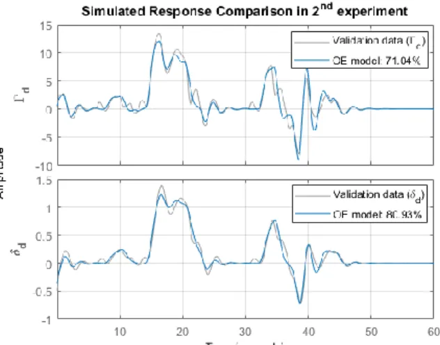
where 𝑦̂ is the simulated response, 𝑦 is the validation data and 𝑦̅ = 𝑚𝑒𝑎𝑛(𝑦). The comparison of outputs and calculation of fit rate for each participant in first experiment and for the simulation data in second experiment are respectively shown in Fig. 11, 12 and 13 (cf. Appendix). The bode diagrams for each OE model identified are shown in Fig. 14 and 15. In Fig. 11 and 12, the outputs of identified OE model issued from road curvature behave like a reference signal for both driver torque and steering wheel angle. The real data from experiments representing drivers’ behaviour changes around these references. This confirms the assumption that the driver will actually try to stay around the reference values sought on the basis of geometric vision with some back and forth behaviour. There is also a large increase in fit percentage between the first and second experiment since the second one uses an a priori identified driver model, which has already eliminated these noises in driver’s behaviour and thus results in a more fitting model compared to validation data.

The bode diagram in first experiment (see Fig. 14) shows a similarity of dynamics between the OE model of female participant and the one of male participant. The bode diagram for the OE model in second experiment (see Fig. 15) shows a narrow confidence region around the identified OE model, which means that the identified model is highly credible.

4. FEEDBACK DESIGN; 𝐻2/𝐻∞ STATIC OUTPUT

FEEDBACK CONTROLLER

The feedback algorithm relies on a output feedback synthesis of a 𝐻2/𝐻∞ command applied on the difference between the

real vehicle-road state, 𝑥𝑣𝑟, and the reference vehicle-road

state, 𝑥𝑟𝑒𝑓. The use of an output feedback allows to select only

measurable values for the feedback instead of having to implement an observer to approximate unmeasurable values as the driver state. The torque command can be written as:

Γ𝑎𝑓𝑏= 𝐾 × 𝑌𝑑𝑖𝑓𝑓= 𝑘𝛽𝛽𝑑𝑖𝑓𝑓+ 𝑘𝑟𝑟𝑑𝑖𝑓𝑓+ 𝑘𝜓_𝐿𝜓_{𝐿 𝑑𝑖𝑓𝑓}+

𝑘𝑦_𝐿𝑦_{𝐿 𝑑𝑖𝑓𝑓}+ 𝑘𝛿_𝑑𝛿_{𝑑𝑑𝑖𝑓𝑓}+ 𝑘𝛿_𝑑̇𝛿𝑑̇ _{𝑑𝑖𝑓𝑓} (3)

with 𝑌𝑑𝑖𝑓𝑓 = 𝑥𝑣𝑟 – 𝑥𝑟𝑒𝑓.

The gain K is found as the solution of the optimization problem described below. Model used to define the optimization problem is shown in Fig. 8. This model can be described by the following equations:

𝑇𝑧𝑤(𝑠) = 𝑇𝑐𝑜𝑚𝑝(𝑠)𝑇𝑡𝑟𝑎𝑗_𝑔𝑒𝑛(𝑠) 𝑤 = [ρ𝑟𝑒𝑓 𝐹𝑤]𝑇, 𝑤𝑡𝑟𝑎𝑗= [Γ𝑎𝑟𝑒𝑓 𝑥𝑟𝑒𝑓 𝜌𝑟𝑒𝑓 𝐹𝑤]𝑇, 𝑧 = 𝑄𝑧[𝜓𝐿 𝑦𝐶𝐺 𝑎 (Γ𝑎− 𝛼𝑐𝑜𝑚𝑝Γ𝑑) Γ𝑑 Γ𝑎] 𝑇 . 𝑤𝑡𝑟𝑎𝑗= 𝑇𝑡𝑟𝑎𝑗_𝑔𝑒𝑛𝑤, 𝑧 = 𝑇𝑐𝑜𝑚𝑝𝑤𝑡𝑟𝑎𝑗,

Where 𝑇𝑐𝑜𝑚𝑝 and 𝑇𝑡𝑟𝑎𝑗_𝑔𝑒𝑛 are the transfer function

corresponding to the rectangle with the same names in Fig. 8, 𝑦𝐶𝐺 is the lateral error of the vehicle’s center of gravity and 𝑎

is the lateral acceleration of the vehicle. 𝑇𝑐𝑜𝑚𝑝 can be

decomposed in column as:

𝑇𝑐𝑜𝑚𝑝= (𝑇Γ𝑎𝑟𝑒𝑓 𝑇𝑥𝑟𝑒𝑓 𝑇𝜌𝑟𝑒𝑓 𝑇𝐹𝑤) with 𝑇Γ𝑎𝑟𝑒𝑓= 𝑄𝑧[𝐶𝑧− Λ1𝐶𝑑𝑣𝑟]Λ2𝐵Γ𝑎, 𝑇𝑥_𝑟𝑒𝑓= 𝑄𝑧Λ1, 𝑇𝜌_𝑟𝑒𝑓= 𝑄𝑧[𝐶𝑧− Λ1𝐶𝑑𝑣𝑟]Λ2𝐵𝜌_𝑟𝑒𝑓, 𝑇𝐹𝑤= 𝑄𝑧[𝐶𝑧− Λ1𝐶𝑑𝑣𝑟]Λ2𝐵𝐹𝑤, Λ1= (𝐶𝑧Λ2𝐵Γ𝑎+ 𝐷𝑧)(𝐼 + 𝐾𝐶𝑑𝑣𝑟Λ2𝐵Γ𝑎) −1 𝐾, Λ2= (𝑝𝐼 − 𝐴𝑑𝑣𝑟)−1,

The 𝐻2 criterion is described using the weighting matrix 𝑄𝑧

defined as: 𝑄𝑧= [ 𝑐1 0 0 0 0 0 0 𝑐2 0 0 0 0 0 0 𝑐3 0 0 0 0 0 0 𝑐4 0 0 0 0 0 0 𝑐5 𝑐𝑑𝑎 0 0 0 0 0 1 ] (4)

In this matrix, parameters 𝑐1, 𝑐2, 𝑐3, 𝑐4, 𝑐5 et 𝑐𝑑𝑎 allow to

weight each criterion according to its importance. 𝑐1 and 𝑐2

are linked to the lane following performance criteria 𝜓𝐿 and

𝑦𝐿. 𝑐3 is linked to a comfort criterion, 𝑎. 𝑐4, 𝑐5 and 𝑐𝑑𝑎 are

linked to the sharing performance criteria Γ𝑎− 𝛼𝑐𝑜𝑚𝑝Γ𝑑, Γ𝑑

and Γ𝑎. 𝑐𝑑𝑎 allows to ensure that the two torques Γ𝑎 and Γ𝑑 are

directed in the same direction.

Fig. 8. Optimization model

The 𝐻∞ criterion is about the system’s stability. It ensures that

the input gain-phase margin 𝑀𝑚𝑖 stays above a limit value.

Knowing that this margin can be written according to the sensitivity function 𝑆𝑖𝑛𝑝𝑢𝑡 as:

𝑀𝑚𝑖= 1 max 𝜔 (|𝑆𝑖𝑛𝑝𝑢𝑡(𝑗𝜔)|) = 1 ‖𝑆𝑖𝑛𝑝𝑢𝑡‖_∞

Then the optimization problem can be written as:

Problem P1: H2 / H∞ static output feedback design

The H2 / H∞ static output feedback design is defined as;

find 𝐾 such that:

- the driver-vehicle-road system is internally stabilized, - is the solution of

𝑚𝑖𝑛𝐾(‖𝑇𝑧𝑤‖2)

under the constraint ‖𝑆𝑖𝑛𝑝𝑢𝑡‖_∞< 𝑆𝑚𝑎𝑥,

with 𝑆𝑚𝑎𝑥 a constant defined a priori.

This optimization is solved using Systune, a tool available in Matlab _{which allows to deal with some non-convex problems}

by using non-smooth optimisation algorithms. 5. SIMULATION AND RESULTS

5.1 Simulation conditions

The shared control strategy was tested by simulating the vehicle-road model (1) driven by the driver model (2) and the assistance. This simulation was done in the Matlab / Simulink

environment. The feedforward is tune as shown in the second experiment in section 3.3.2. The vehicle-road model used for the simulation is the same that the one used to synthetized the feedback. The simulation was done by following the road depicted in Fig. 6 and curves curvature along the road goes from 0.002 𝑚−1 _{to 0.038 𝑚}−1_{. The longitudinal speed of the}

vehicle is fixed at 𝑉𝑥 =18 m/s. The wind disturbance input 𝐹𝑤

is not taken into consideration. Coefficients of the matrix 𝑄𝑧

(4) are chosen as 𝑐1= 200, 𝑐2= 20, 𝑐3= 3, 𝑐4= 10, 𝑐5= 1

and 𝑐𝑑𝑎= −10. The minimum value for the input modulo

margin 𝑀𝑚𝑖 is 0.5. Both level of sharing 𝛼𝑎𝑛𝑡 and 𝛼𝑐𝑜𝑚𝑝 are

chosen equal to 50%.

5.2 Performance indicators

In order to assess the control strategy developed here in terms of sharing performances, some indicators which were introduced in (Saleh et al., 2013) and (Saleh et al., 2010) :

- Consistency ratio, 𝑇𝑐𝑜, defined as the duration during

which assistance torque Γ𝑎 is in the same direction as

the driver torque Γ𝑑 divided by simulation’s duration.

- Resistance ratio, 𝑇𝑟𝑒𝑠, defined as the duration during

which assistance torque Γ𝑎 and driver torque Γ𝑑 are in

opposite direction and assistance torque is inferior or equal to the driver torque divided by simulation’s duration

- Contradiction ratio, 𝑇𝑐𝑜𝑛𝑡, defined as the duration

during which assistance torque Γ𝑎 and driver torque Γ𝑑

are in opposite direction and assistance torque is higher than the driver torque divided by simulation’s duration. - Sharing level that is defined as the effort produced by the assistance divided by the effort produced by the driver 𝑃𝑚= 𝐸𝑎 𝐸𝑑 =∫ Γ𝑎 2_{(𝑡)𝑑𝑡} ∞ 0 ∫ Γ𝑑2(𝑡)𝑑𝑡 ∞ 0

- Coherence level that is the cosine value of the angle between the assistance torque and the driver torque

𝑃𝑐 = cos(Γ⃗⃗⃗ , Γ𝑎 ⃗⃗⃗ ) =𝑑 ∫ Γ𝑎(𝑡) × Γ𝑑(𝑡)𝑑𝑡 ∞ 0 √∫ Γ𝑎2(𝑡)𝑑𝑡 ∞ 0 × ∫ Γ𝑑2(𝑡)𝑑𝑡 ∞ 0

The lane following performances are assess using the average, the maximal and the standard deviation of the lateral error.

5.3 Results

First the design of the feedback part resulted in an input module margin of 0.505 which is higher than the minimal value 0.5.

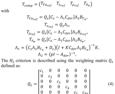
Results found during the simulation are shown in Fig. 9, Fig. 10 and Table 2. The first figure shows that the assistance is, most of the time, helpful for the driver. It applied a part of the steering torque, allowing the driver to apply less effort on the steering wheel to steer the vehicle.

Fig. 9 : Torque command applied by the driver and the assistance

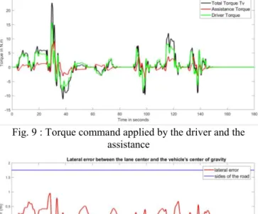
Fig. 10 : Lateral error between the lane centre and the vehicle’s centre of gravity during the simulation

Table 2. Simulation results

Indicators Results

max(lateral_error)(m)

average(lateral_error)(m)

Std(lateral_error)(m)

𝑇

𝑇

𝑇

𝑃

𝑃

However, it has to be said that the track used here presents a very tight bend which can be noticed on Fig. 6, leading at about 30s to unusual torque and lateral error. These results are not representative as the track is not inclined and the speed is too high to be realistic.

Table 2 and Fig. 10 show good lane following performances, with a low lateral error, which average value is 0.22m. Table 2. also shows good results in terms of sharing performance. Indeed, the consistency ratio is close to the one found in (Saleh et al., 2013), that used an LQ with preview theory to design a shared lateral control, based on a cybernetic driver model-vehicle-road model. The resistance ratio is equal to 0.41; this value may seem high, but the assistance resists to the driver action mostly in situations during which the torque applied both by the assistance and the driver are very low so it is not noticeable for the driver; to a lesser extent, some resistance occurs during the transition period at the beginning of bends. Considering now the contradiction ratio, it is even lower than the one found in (Saleh et al., 2013) which is remarkable because it corresponds to a frontal conflict between the driver and the assistance. Finally, the coherence level 𝑃𝑐 is positive

which means that the driver and the assistance applied a torque in the same direction most of the time.

6. CONCLUSION

This paper described a haptic shared control strategy. It proceeded sequentially, considering first the feedforward, and then the feedback based on both the feedforward generator and the cybernetic driver model. This feedforward uses a dynamic model able to predict the torque that should be applied on the steering wheel consistently with the road geometry (curvature). This model is obtained by identification, from experimental data measured on a driving simulator with a real driver. This identification in fact proceeded to a projection of the “geometric part” of human driving, on a second order model with the road curvature as input, and the steering torque and all the vehicle-road states as outputs. Outputs of this model were then used as reference trajectory generator to design the haptic shared control proposed. The feedback relies on a 𝐻2/𝐻∞ output feedback applied on the difference between the

real vehicle-road state and the reference one. Criteria used to design the feedback gains are concerned with lane following performances as well as the quality of sharing between the assistance and the driver, with an evaluation involving a cybernetic driver model. Both feedforward and feedback parts were then designed sequentially leading to nice results on performance aspects with complementary actions between the assistance and the driver.

This study opens interesting perspectives deserving to be studied in depth. Among them, the authors will realize experiments from significant samples of drivers, first on driving simulator. A joint analysis of the results obtained both objectively and subjectively will be made, according to drivers feelings about the shared control tested.

ACKNOWLEDGMENTS

This work was supported by AutoConduct research program funded by the French ANR “Agence Nationale de la Recherche” (grant ANR-16-CE22-0007-05), and RFI Atlanstic 2020, funded by the Region Pays de la Loire.

REFERENCES

Abbink, D.A., Carlson, T., Mulder, M., Winter, J.C.F. de, Aminravan, F., Gibo, T.L., Boer, E.R., (2018). A Topology of Shared Control Systems—Finding Common Ground in Diversity. IEEE Transactions on

Human-Machine Systems, 48, 509–525.

Abbink, D.A., Cleij, D., Mulder, M., Paassen, M.M. v, (2012). The importance of including knowledge of neuromuscular behaviour in haptic shared control.

IEEE International Conference on Systems, Man, and Cybernetics (SMC). 3350–3355.

Ameyoe, A., Chevrel, P., Le-Carpentier, E., Mars, F., Illy, H., (2015). Identification of a Linear Parameter Varying Driver Model for the Detection of Distraction. In 1st

IFAC Workshop on Linear Parameter Varying Systems LPVS 48, 37–42.

Attia, R., Daniel, J., Lauffenburger, J.P., Orjuela, R., Basset, M., (2012). Reference generation and control strategy for automated vehicle guidance. IEEE Intelligent

Vehicles Symposium, 389–394.

Benloucif, M.A., Sentouh, C., Floris, J., Simon, P., Popieul, J.-C., (2017). Online adaptation of the Level of Haptic Authority in a lane keeping system considering the driver’s state. Transportation Research Part F:

Traffic Psychology and Behaviour.

Blaschke, C., Breyer, F., Färber, B., Freyer, J., Limbacher, R., (2009). Driver distraction based lane-keeping assistance. Transportation Research Part F: Traffic

Psychology and Behaviour 12, 288–299.

Griffiths, P., Gillespie, R.B., (2004). Shared control between human and machine: haptic display of automation during manual control of vehicle heading. 12th

International Symposium on Haptic Interfaces for Virtual Environment and Teleoperator Systems. HAPTICS ’04. Proceedings, 358–366.

Hermannstädter, P., Yang, B., (2013). Driver Distraction Assessment Using Driver Modeling. IEEE

International Conference on Systems, Man, and Cybernetics, 3693–3698.

Kapania, N.R., Gerdes, J.C., (2015). Design of a feedback-feedforward steering controller for accurate path tracking and stability at the limits of handling.

Vehicle System Dynamics 53, 1687–1704.

Kuwata, Y., Teo, J., Karaman, S., Fiore, G., Frazzoli, E., How, J., (2008). Motion Planning in Complex Environments Using Closed-loop Prediction. AIAA

Guidance, Navigation and Control Conference and Exhibit,

Ljung, L., (1999). System Identification Theory for the User

(2nd _{ed.). Prentice-Hall PTR.}

Mars, F., Chevrel, P., (2017). Modelling human control of steering for the design of advanced driver assistance systems. Annual Reviews in Control 44, 292–302.

Mugge, W., Kuling, I.A., Brenner, E., Smeets, J.B.J., (2016). Haptic Guidance Needs to Be Intuitive Not Just Informative to Improve Human Motor Accuracy.

PLOS ONE 11, e0150912.

Saleh, L., (2012). Contrôle Latéral Partagé d’un Véhicule Automobile (phdthesis). Ecole Centrale de Nantes (ECN).

Saleh, L., Chevrel, P., Claveau, F., Lafay, J., Mars, F., (2013). Shared Steering Control Between a Driver and an Automation: Stability in the Presence of Driver Behavior Uncertainty. IEEE Transactions on

Intelligent Transportation Systems 14, 974–983.

Saleh, L., Chevrel, P., Lafay, J.-F., (2010). Generalized H2-Preview Control and its Application to Car Lateral Steering. 9th IFAC Workshop on Time Delay Systems 43, 132–137.

Saleh, L., Chevrel, P., Mars, F., Lafay, J.-F., Claveau, F., (2011). Human-like cybernetic driver model for lane keeping. 18th IFAC World Congress 44, 4368–4373. Sentouh, C., Chevrel, P., Mars, F., Claveau, F., (2009). A

sensorimotor driver model for steering control. IEEE

International Conference on Systems, Man and Cybernetics, 2462–2467.

Rajamani, R., (2012). Vehicle Dynamics and Control. Springer, New York, NY, USA

Appendix A. IDENTIFICATION FIGURES

Fig. 11. Validation data vs. OE model, female participant

Fig. 12. Validation data vs. OE model, male participant

Fig. 13. Validation data vs. OE model, 2nd _experiment

Fig. 14. Bode diagram of OE model in 1st _experiment