HAL Id: hal-01923540
https://hal.archives-ouvertes.fr/hal-01923540
Submitted on 26 Nov 2018
HAL is a multi-disciplinary open access
archive for the deposit and dissemination of
sci-entific research documents, whether they are
pub-lished or not. The documents may come from
teaching and research institutions in France or
abroad, or from public or private research centers.
L’archive ouverte pluridisciplinaire HAL, est
destinée au dépôt et à la diffusion de documents
scientifiques de niveau recherche, publiés ou non,
émanant des établissements d’enseignement et de
recherche français ou étrangers, des laboratoires
publics ou privés.
Statistical investigation of different analysis methods for
chloride profiles within a real structure in a marine
environment
Inès Othmen, Stéphanie Bonnet, Franck Schoefs
To cite this version:
Inès Othmen, Stéphanie Bonnet, Franck Schoefs. Statistical investigation of different analysis methods
for chloride profiles within a real structure in a marine environment. Ocean Engineering, Elsevier,
2018, 157, pp.96 - 107. �10.1016/j.oceaneng.2018.03.040�. �hal-01923540�
1
Investigation of different analysis methods for chloride profiles within a real structure in a marine
1
environment
2
Ines.Othmen
a,1, Stéphanie Bonnet
b, Franck Schoefs
a3
a
UBL, Université de Nantes, GeM, CNRS UMR 6183, 2 rue de la Houssinière (BP 92208), 44322 Nantes
4
Cedex 03, France
5
b
UBL, Université de Nantes, GeM, CNRS UMR 6183, 58 rue Michel Ange (BP420), 44606 Saint Nazaire
6
Cedex, France
7 1Corresponding author.
8E-mail: [email protected]
9Tel : +33 (0)2 53 48 73 02
10 Abstract 11Corrosion is a major problem for durability of reinforced concrete structures in a marine environment. To 12
establish the best accurate planning for maintenance operations, assessing chloride ingress within concrete is 13
essential. The present paper reports a study conducted to investigate a large amount of field chloride data 14
collected from a 28-years old beam in a splash zone. The chloride profiles are examined based on Fick’s second 15
law to estimate the surface content Cs and the diffusion coefficient D. Firstly, three different cases considering
16
the location of the maximum chloride content are tested: a reference case (individual analysis), a 15-mm 17
discarded case and a 20-mm discarded case (generic treatments). The results highlight the importance of the 18
individual analysis. Cs and D, indeed, appear to be significantly affected by the generic treatment, the relative
19
error being around 50% for Cs and 100% for D. A focus is therefore placed on the individual analysis. The
20
coefficients of variation are 44% and 61% for Cs and D, respectively. For the statistical distribution, both
21
parameters show a clear dependence. They also follow a lognormal law with a mean value ranging between 22
0.0057 and 0.0085 kgCl-/ kgconcrete for Cs and equal to 1.3x10⁻¹² m²/s for D.
23
Key words: reinforced concrete, splash zone, chloride profiles, individual treatment, generic treatment,
24
statistical analysis 25
2 27
1. Introduction 28
Chloride penetration into concrete can cause irreversible damage within reinforced concrete structures, 29
predominantly corrosion damage, when chloride content at the surface of reinforcement bars reaches a certain 30
threshold level. Steel corrosion initiation is then a key indicator for the estimation of service life. The risk of 31
corrosion damage is higher in a marine environment because of significant humidity and chloride contents in 32
both seawater and air. Consequently, the corrosion of engineering structures is more severe in coastal areas than 33
inland locations (Guo et al., 2015). Chloride profile analysis, is therefore, an important tool for service life 34
predictions of structures and inspection/maintenance/repair action scheduling (Bastidas-Arteaga et al., 2011; de 35
Rincón et al., 2004). Recent studies have highlighted the spatial variability of chloride-induced reinforced 36
concrete corrosion with an impact on infrastructure network maintenance optimization (O’Connor and Kenshel, 37
2013). In the following, the focus is on total chloride content because, firstly, measurement methodology is not 38
subject to debate (Bonnet et al., 2017) and, secondly, because it is the key parameter for already available 39
maintenance optimisation methods. 40
Chloride profile analysis is therefore essential. Profiles are better assessed when different factors like concrete 41
properties (Tadayon et al., 2016) and period of exposure (Mangat and Molloy, 1994, Tamimi et al., 2008) are 42
taken into account. Exposure (above sea level: atmospheric and splashing zones, and under sea level: tidal and 43
immersed zones) and environmental conditions (temperature, relative humidity, wind, orientation…) are also 44
important factors in affecting the durability of concrete and in shortening the life span of structures. Many 45
studies have shown that tidal and splash zones drive the most severe conditions as regards chloride ingress and 46
steel corrosion of concrete in comparison with atmosphere and immersed zones (Valipour et al., 2013). Li and
47
Shao (2014) conclude that immersed zones allow for a service life 1.6 to 3.9 times longer than splash zones, 48
whatever the binding isotherm considered. Furthermore, in marineexposure conditions, chloride ions can 49
penetrate into concrete through multiple mechanisms including diffusion, adsorption, permeation and surface 50
deposit of airborne salts (Hilsdorf and Kropp, 2004). Although chloride ingress within concrete involves many 51
mechanisms, it is widely accepted that diffusion is the primary mechanism (Pang and Li, 2016). Hence, chloride
52
ingress can be modelled by the empirical Fick’s diffusion model. Besides, The Fick’s model is used by engineers
53
and researchers to deal with in situ data (see references on table 1) and recommended by codes like Fédération
54
International du Béton (2006) for its simplicity and its capacity of being adapted to different exposure cases.
3
Indeed, a comparison of an oversimplified model to an improved model shows that both yields to similar results
56
(Nguyen et al., 2017) and fairly well predict the chloride ingress in a Portland cement (up to 100 years) (Luping
57
and Gulikers, 2007). Moreover, a long-term monitoring on real concrete structures exposed to environmental
58
conditions makes the empirical Fick’s model adapted for durability design (Li et al., 2015).
59
Then, many studies have been devoted to the measurement of chloride ingress within real structures like decks, 60
piles, offshore platform or concrete specimens, in a marine environment with different exposure conditions 61
(Table 1). The chloride profiles obtained (often) have the shape of a bell with a chloride content, which increases 62
from the concrete surface to a certain depth where a maximum content, noted Cpeak in Table 1, is reached and
63
then decreases as depth increases. This is accounted for by (Andrade et al., 1997) as “concrete surface skin 64
effect”. In the studies reported in Table 1, the approach commonly used to estimate both surface content Cs and
65
diffusion coefficient D come from the fitting of the Fick’s second law to in-situ values of experimental chloride
66
profiles. This regression beginning at Cpeak provides Cs and D simultaneously.
67
It should be noted that the value of Cpeak varies from 0.0014 kgCl-/kgconcrete (Pang and Li, 2016) to 0.013
68
kgCl/kgconcrete (Chalee et al., 2009). Cpeak can also start at 0 mm (Chalee et al., 2009; de Rincón et al., 2004),
69
around 10 mm (Medeiros-Junior et al., 2015; Pang and Li, 2016; Thomas and Matthews, 2004), and at 20 mm or 70
30 mm (de Rincón et al., 2004). The depth may vary in relation to concrete quality, exposure conditions and 71
structure orientation. Some values of D obtained vary between 0.27 x 10⁻¹² m²/s (da Costa et al., 2013) and 72
5.13 x 10⁻¹² m²/s (Medeiros-Junior et al., 2015). 73
Among key parameters and phenomena (quality of concrete, exposure conditions and orientation) affecting 74
structure service life, exposure conditions are the focus of this research. The present paper, indeed, reports the 75
experimental investigation carried out on a 28-years old beam made from the same concrete composition and on 76
which all the chloride profiles are measured on the same horizontal line (coring is performed on the same line 77
along the beam). Moreover, the studied beam is located in a splash zone influenced by two local microclimates 78
(both beam exposures are detailed in §2.1). The present study also provides a significant number of chloride 79
profiles in accordance with (Medeiros-Junior et al., 2015), who underline the significance of the number of 80
samples as a direct benefit to achieve precise statements. Furthermore, De Vera G. et al. (2015) highlighted that
81
to assign reliable values for CS it is only possible on the basis of experimental chloride profiles obtained with the
82
similar concrete composition and in similar locations. As for D, the sensitivity analysis realised by Li et al.
4
(2009) shows that the achieved reliability of design is rather sensitive to the mean of D values as well as the
84
cover thickness. It is thus necessary to evaluate D accurately.
85
These data form a substantial high value data base to improve the scientific documented knowledge library for 86
concrete subject to XS3 class environmental exposure according to the NF EN 206-1 standard. The objective of 87
this research is to address the problem of the determination of Cs that usually results from the chloride content
88
reduction at the concrete surface (Song et al., 2008). So, the variation of the position where Cpeak is measured
89
appears to constitute a possible alternative route for study. 90
Thus, this paper provides an important data base of chloride measurements done on the same beam with reduced
91
settings like concrete composition, location, marine environment and tidal height that were all the same for 30
92
core samples. Indeed, approximately 600 chloride measurements were carried out to highlight the observations
93
and comments done hereafter. On a comparable data, it is possible, on the one hand, to underline the variability
94
of the raw data of chloride profiles and, on the other hand, the variability of Cs and D along the beam once the
95
raw data was processed by Fick’s second law solution. This work, as far as we know, has never been done on so
96
many data.
97
Since very numerous comparable data are available it led us to review the generic treatment used by some
98
authors to deal with chloride profiles to determine Cs and D (Chalee et al., 2009; da Costa et al., 2013; Pang and
99
Li, 2016).This treatment was compared to the individual treatment called reference case in this paper which is
100
more time consuming than the previous treatment. 101
Accordingly, the paper is structured as follows: 102
- Experimental investigation of the studied structure.
103
- Experimental chloride profile fitting methodology based on three sets of analyses depending on the
104
chloride maximum content position and using Fick’s second law to assess Cs and D.
105
- Cs and D results presentation for the three sets of analyses. The focus is made on the reference case to
106
derive the statistical distribution and the covariance. 107
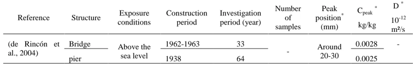
Table 1: Peak values of total**chloride content and diffusion coefficient of concrete structures and specimens exposed to a marine environment
Reference Structure Exposure
conditions Construction period Investigation period (year) Number of samples Peak position* (mm) Cpeak* kg/kg D * 10-12 m²/s (de Rincón et al., 2004)
Bridge Above the
sea level 1962-1963 33 - Around 20-30 0.0028 - pier 1938 64 0.0025
5
bridge 1986 11 0 0.0018
(da Costa et al., 2013). Offshore oil platform Wetting drying cycles 25 35 Around 10-20 0.0029 : 0.0051 0.27 : 1.6 (Chalee et al., 2009) Cube specimens (in sea water)
Two wet dry cycles of sea water daily
- 5 - 0 mm 0.013 1.65
(Pang and Li, 2016)
Pile wharf structure
splash zone between
1971 and 2008 36 8/pile 14 piles tested Between 0 and 10 0.0046 0.35 (Medeiros-Junior et al., 2015) Offshore platform
splash zone 1976 29 3 layers/
point of investi-gation 10 0.007 5.13 (Thomas and Matthews, 2004) Cube specimens (in sea water)
Tidal zone - 1, 2 and 10 - around
7.5 -10 0.0038 : 0.006 - (Pritzl et al., 2015) Deck bridge deicing salt environment Between 1992 and 1995 16 4 locations 10 0.0059 2 (Tadayon et al., 2016) Cube specimens (in sea water) Tidal zone - 4.17 (=50 months) - 2.5 0.006: 0.0091 2:4.2 (Cramer et al., 2002) bridge Marine breeze - 40 to 60 - - 0.0073 : 0.003 0.41: 1.71
(Kenshel, 2009) pier Atmospheric
zone 1980 27 45 Between 10 and 25 mm 0.0004 : 0.0013 0.098 : 0.72 *
Peak position is the position within the sample where the maximum chloride content (Cpeak) is measured. When information are missing to 108
convert C and D into kg/kg and m²/s, respectively, we considered Cement concentration =350kg/m3 and concrete bulk density =2500kg/m3 109
**except for Medeiros-Junior et al., 2015 where only free chloride content is measured 110
2. Experimental investigation of the studied structure 111
2.1. Test Area 112
Harbour infrastructures, especially energy-related ones, are important components of the transportation system in 113
coastal areas. We, therefore, focus on the coal terminal of the test area. The coal terminal is located within the 114
industrial and port activity area, which includes many specialised facilities near the city of Saint-Nazaire 115
(France). The coal terminal, which is one of the largest thermal power stations in Europe, is used for the import 116
and then the transportation of coal by inland waterways to support French power supply. 117
The coal terminal (Fig. 2a), built between 1981 and 1983, consists of five bridge piers (54.5m in length *9.8 m 118
in width each) giving access to an unloading platform (246.4 m in length* 20.7 m in width). 119
6 For accessibility reasons, the study is conducted on beam J of Pier 5 (Fig. 1b). The beam is 9.35m long and 120
0.40m wide. The upstream side, exposed to weather variations, is called “exposed side” (noted ES) whereas the 121
protected downstream face being situated in a confined environment is called “sheltered side” (noted SS) (Fig. 122
1c and Fig. 1d). Beam J is located in the estuary area of the Loire River less than 7 km from the Atlantic Ocean. 123
The beam is situated 5.8 m above sea level, in a splash zone where the bottom of the beam may be in contact 124
with seawater when tidal coefficients are high (roughly 2 days/month). The climatic data, including temperature 125
(T), relative humidity (RH) and wind speed, cumulative rainfall and the atmospheric pressure (P), have been 126
recorded by the French Government weather station1 near the Saint-Nazaire harbour (Table 2). Temperature 127
mean maximal and minimal values are 16.9°C and 8.7°C, respectively, with high relative humidity (>80%). 128
Table 2: Climatic data of the beam surrounding environment Mean max T [°C] Mean min T [°C] Mean RH [%] Maximal Wind speed [km/h] Cumulative Rainfall [mm] Max rainfall per 24h [mm] Max P [hPa] Min P [hPa] Mean value (between 1981 and 2011) 16.9 8.7 >80% 133.3 788.6 61.8 961.6 1088 129 a) b) c) d) 1 http://www.infoclimat.fr/stations-meteo/climato-moyennes-records. N
Pier 3 Pier 4 Pier 5
Atlantic Ocean Loire estuary
Sheltered side Exposed side
40 cm
Exposed side
7 Fig. 1: Coal terminal a) aerial view b) sketch of bridges 3,4 and 5 c) Picture of beam J d) Exposed and sheltered sides of beam J
2.2. Concrete composition 130
When studying the existing documentation from the coal terminal, we find some data available about the 131
concrete. It is a Portland cement where clinkers make up more than 90% of the cement and secondary
132
constituents shall not exceed 5%. The cement has also a strength class of 45 MPa . The aggregates used are sand 133
0/6 and gravel 5/10 and 10/25. The cement content of 350kg/m3 is specified but not aggregate and water 134
contents. 135
Concrete open water porosity and compressive strength are both measured on the central parts of the extracted 136
cores that were sawn and rectified to obtain a flat surface (slide Number 3 in Fig. 2c). 137
Concrete cylinders were oven-dried at 60 °C until reaching constant weight. Then they were cooled for 48 h in a
138
desiccator at 20 °C before being water saturated to determine their open water porosity(Ben Fraj et al., 2012).
139
The porosity is obtained from five samples with a mean value of 13.7% (min value =11.3% and max value 140
=15.9%). The compressive strength is obtained from four 5-cm diameter and 10-cm long samples. The loading 141
speed was of 5kN/s. The mean value is 43.5MPa (min value =38.5MPa and max value =48.9MPa). 142
2.3. Experimental investigation for chloride content 143
The extraction of the cylindrical cores took place in 2011 after 28 years of exposure and carried out along a line 144
situated 30 cm above the bottom of the beam. Thirty samples have been collected every 30 cm (red dots in Fig. 145
2a) and numbered from 1 to 30 from the Loire estuary side to the embankment side of the beam. 146
a)
A A
8
b) c)
Fig. 2: Investigation line a) front view with cores positions b) cross section A-A and c) sample diagram The thirty specimens are cylinders 5 cm in diameter and 40 cm in length. Each core is cut into five slices: slices 147
1 and 2 correspond to the exposed side (ES) and slices 4 and 5 to the sheltered side (SS) (Fig. 2c). All are used to 148
determine the chloride profiles. Slice n°3 is used for other investigations like porosity and compressive strength 149
(§2.2) and for the determination of the initial chloride content (§3.2). 150
The procedure recommended by the RILEM Technical Committee 178-TMC (“Recommendation for analysis of 151
total chloride in concrete.,” 2006) is followed to obtain the chloride profiles. Slices are grounded first into 5-mm 152
thick layers up to a depth of 5 cm (slices 1 and 5 in Fig. 2c) and then into 10-mm thick layers for the remaining 5 153
cm (slices 2 and 4 in Fig. 2c). This method makes it possible to monitor the progression of the fitting and to 154
assess the peak position on the profile with good accuracy (+/-2.5 mm), the other parts of the core (# 2 and #4) 155
having less impact on the fitting accuracy. For the recovery of powder, grounding is made perpendicularly to the 156
top faces of the cylinders using a grinding instrument as recommended by Vennesland (Vennesland et al., 2012). 157
The powder is collected and stored in sealed plastic bags. The procedure described below is used to determine 158
the total chloride content from concrete powder (Chaussadent and Arliguie, 1999; Vennesland et al., 2012). 159
In order to extract the chloride from the concrete powder samples, 100 ml of nitric acid is added to 5 g of 160
grounded concrete powder. The mixture is heated and stirred for 30 min. The solution obtained is then filtered 161
into a 250-cm3 volumetric flash. The chloride content of the filtered solutions is finally determined by 162
potentiometric titration using an automatic titrator with 0.05-M silver nitrate (AgNO3) as titrant.
163
3. Fitting method 164
3.1. Chloride profiles 165
The chloride content is plotted as a function of the distance (in mm) from the top surface for both sides (SS and 166
ES) to illustrate chloride profiles. Samples are numbered from 1 to 30 as shown in Fig. 2a. 37 workable profiles 167
9 are thus obtained, which are distributed as follows: 21 profiles from the sheltered side (SS) and 16 profiles from 168
the exposed side (ES). The profiles are summarized in Table 3 (cross mark means availability). 169
Missing profiles 9, 11, 12 and 26 correspond to the cores damaged during sampling. Other profiles have also 170
been eliminated. Indeed, when plotting chloride concentrations as a function of depth, some profiles present a 171
linear trend suggesting the presence of cracks that may trap a significant amount of chloride (Erreur ! Source 172
du renvoi introuvable.–curves with empty markers).
173
Wang et al. (2016) have examined the effects of different crack parameters on the chloride diffusion into 174
concrete and have demonstrated that it highly depends on the crack density (represents the amount of cracks), in 175
addition to crack width and crack tortuosity. 176
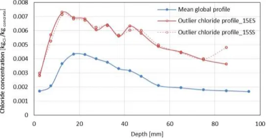
An outlier reveals a very high chloride content in the chloride profile, which should then be discarded. The 177
discarded profiles here are 3, 15 17, 20 and 29 on the sheltered side and 3, 6, 7, 8, 9, 15, 17, 20, 22 and 29 on the 178
exposed side. 37 profiles are finally processed. The mean global profile, represented as the mean chloride 179
content for both sides (mean of the 37 profiles), is given in Fig. 3 (blue solid line). 180
181
Fig. 3: Example of profiles with outliers (high values of concentration) with respect to the global mean profile 182
Table 3: Summary of the profiles obtained
Sample Position (cm) SS ES Sample Position (cm) SS ES Sample Position (cm) SS ES
1 20 11 320 21 620
2 50 12 350 22 650
3 80 13 380 23 680
4 110 14 410 24 710
10 6 170 16 470 26 770 7 200 17 500 27 800 8 230 18 530 28 830 9 260 19 560 29 860 10 290 20 590 30 890
For the sake of clarity, only mean chloride ingress profiles and error bars corresponding to standard deviation are 183
presented in Fig. 4 for both exposures. The mean value is calculated for both sides from the retained 184
experimental profiles (21 and 16 profiles for SS and ES, respectively). It ought to be pointed out that the number 185
of profiles is very high and composes a substantial high value data base that can be used to estimate low order 186
statistics (mean and standard deviation) with a low statistical uncertainty. It should also be reminded here that all 187
the chloride profiles studied come from the same structure, with the same concrete material and the same 188
environmental conditions (constant height above sea level, orientation, exposure, etc.). However, despite this, all 189
the points of the profiles display a high standard deviation. 190
Fig. 4: Mean chloride profiles for both exposures (SS and ES) and for the central point (used as initial chloride 191
content) 192
The chloride profiles from both sides of the beam (SS and ES) reveal identical behaviour: first, a low chloride 193
content at the concrete surface, which increases to a peak value (around 20 mm for the mean profile) and then 194
decreases to the central point (estimated from eight samples and corresponding to slice n°3 on Fig. 2c). Then the 195
chloride profiles reveal the well-known bell shape as it appears in many researches (Song et al., 2008; Win et al., 196
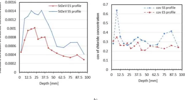
2004). It should also be noted that the standard deviation values are higher and more variable on the sheltered 197
side (Fig. 5a) and that they remain lower than 0.000156, the upper bound of the standard deviation of the error 198
on chloride measurements calculated by Bonnet et al. (2017). Moreover, the lower the chloride content, the 199
11 smaller the standard deviation. This observation may be accounted for by the fact that high chloride content is 200
affected by a combination of several factors, which are very changeable along the beam due to the environment 201
or to the heterogeneity of concrete during processing (vibration). The coefficient of variation is similar on both 202
sides with most values within the range 0.25-0.35, save near the beam surface (Fig. 5b). This confirms an 203
interesting statistical property for probabilistic modelling: the higher the chloride content, the higher the 204
uncertainty. Duprat (2007) has shown that a high degree of uncertainty combined with some environmental 205
parameters makes the chloride intake unpredictable. Chloride content values, on the other hand, are higher on the 206
sheltered side because the concrete beam stands in a confined environment, highly loaded with salt spray. 207
Chloride ions are trapped beneath the slab. 208
a) b)
Fig. 5: a) Standard Deviation (StDev) and b) coefficient of variation (COV) for chloride content for both exposures
3.2. Analytical model for diffusion law 209
In a marine environment, concrete can be considered as almost saturated. Indeed, the concrete used for the
210
studied beam was casted in-situ. Thus, it was initially saturated and persistently exposed to high RH. RH ,
211
superior to 80%, as shown in Table 2 was measured according to a national meteo station located nearby the
212
beam but not so closed to the sea water as this one. Moreover the beam is submitted to water coming from
213
splashing and/or rain. Besides, the pore network of the cement matrix is very thin. Baroghel-Bouny et al. (1999)
214
explained that in this case the water displacement into concrete is low and can be described by a diffusion
215
equation.
12
. Thus,chloride ingress is modelled using Fick’s diffusion model except near the surface and it is applied to fit 217
the experimental chloride profiles. 218
For a homogeneous concrete, a constant surface content and a one- dimensional diffusion into a semi-infinite 219
space, Fick’s second law is expressed as: 220
(1)
where C is the chloride content at a depth of x (m) after time t (s); C0 (kgCl-/kgconcrete) the initial chloride content
221
in concrete before exposure, Cs (kgCl-/kgconcrete) the chloride content at the surface and D (m²/s) the diffusion
222
coefficient. 223
The initial chloride content C0 is obtained from eight samples at a depth of 200mm, which is considered distant
224
enough from the surface to be representative of uncontaminated concrete. A very low negligible coefficient of 225
variation (less than 2%) is obtained with a mean value C0=0.001019 kgCl-/ kgconcrete, a maximum value= 0.001066
226
kgCl-/kgconcrete and a minimum value= 0.000964 kgCl-/kgconcrete. The mean value is subsequently used. Besides Cs
227
and D are not time dependant in the paper, as it was done by (Chalee et al., 2009; Tadayon et al., 2016; Valipour
228
et al., 2013), since all the samples have been taken from the same beam at the same age of 28 years old.
229
Moreover it was showm by Ben Fraj et al. (2012) that the diffusion coefficient decreases particularly in the first
230
few months. The values for Cs and D were provided simultaneously by fitting the experimental profiles with Eq.1
231
and wereobtained by iteration using the Mathematica software with the least square minimization method 232
3.3. Fitting method 233
C0 being known, the estimation of parameters Cs and D of Fick’s second law by fitting the experimental chloride
234
profiles implies that these profiles have a monotonic decreasing shape. This is not, however, the case near the 235
concrete surface where the first few centimetres present a high positive chloride gradient (Fig. 4). That is why 236
discarding the first few centimetres below the surface is a commonly used technique (Chalee et al., 2009; Pang 237
and Li, 2016). Da Costa et al. (2013) specify that the aim in doing this is to eliminate lixiviation effect. 238
Moreover, Fig. 6a shows that peak positions (the depth corresponding to the maximal chloride concentration) 239
occurs at different depths between 12.5 mm and 37.5 mm with a maximum occurrence within the range 12.5 mm 240
- 22.5 mm. The objective of the following section is to examine the effect of pre-treatment (discarding of 241
experimental data close to the surface) on the estimation of the Fick’s law parameters. We will compare some 242
13 generic treatments (Cases 2 and 3) commonly used in various research works with the individual treatment (Case 243
1), which is specific to each chloride profile; the objective is here to evaluate the relevance of the latter. 244
a) b)
Fig. 6: a) Distribution of peak positions (relative to the concrete surface) along the beam and b) Frequency of the peak positions
The three different experimental data pre-treatments studied here are now described: 245
- In the first case, called “reference case”, the treated profiles start from the real peak value that varies 246
from a sample to another (no assumption is required). This method, where the peak position is assumed to be a 247
random variable, is in better agreement with the real evolution of data. The trend, indeed, is a decreasing one 248
(Bastidas et al, 2011, Nilsson et al., 2010). The peak value position varies within the range 12.5 mm - 37.5 mm 249
(Fig. 6). The pre-treatment of the experimental profiles is then carried out on an individual basis. 250
The two other treatments can be carried out on a systematic basis, relying, however, on the assumption of the 251
peak position, which is assumed here to be deterministic: 252
- In the second case “15-mm discarded case”, all data from the first 15 mm below the concrete surface
253
are discarded. All the profiles start with the data at abscissa 17.5 mm, which corresponds to a recurrent 254
frequency peak depth for both exposed and sheltered sides (n=11 in Fig. 6b). Moreover, the maximum absolute 255
deviation between the real peak value (corresponding to the starting point in the reference case-1) and the value 256
at 17.5 mm is 0.0022 kgCl-/ kgconcrete for the sheltered side and 0.0012 kgCl-/ kgconcrete for the exposed side.
257
- In the third case” 20-mm discarded case”, all data from the first 20 mm below the concrete surface are
258
discarded. The profiles here start at abscissa 22.5 mm, which is the highest peak position frequency for both the 259
sheltered and the exposed sides (n=15 for SS and 5 for ES in Fig. 6b). Moreover, the maximum absolute 260
14 deviation between the real peak value and the value at 22.5 mm is 0.0014 kgCl-/ kgconcrete for the sheltered side
261
and 0.0015 kgCl/ kgconcrete for the exposed side.
262
4. Results and discussion 263
4.1. Preliminary comparison of the three pre-treatments 264
The 37 experimental profiles are fitted using Fick’s second law (Eq. 1) with the three pre-treatments to estimate 265
Cs and D parameters. The main trends emerging from the results are discussed on the basis of the study of three
266
profiles. Fig. 7 illustrates the fitting for three profiles with different real peak positions: 12.5 mm (profile 1ES), 267
17.5 mm (profile 14ES) and 22.5 mm. (profile 4ES). The analysis of the shape of the curves, which can indicate 268
the trend for (i) Cs and (ii) D, is then conducted. The quantitative results are displayed in Table 4 where the
269
relative error (RE) is defined as 270
RE =(y-yref)/yref (2)
where y is Cs or D for the two pre-treatment cases (discarded 15 mm and 20 mm, respectively), yref is Cs or D for
271
the reference case. 272
(i) The estimation of the surface chloride content is first examined. For most specimens, pre-treatments 2 273
and 3 underestimate Cs. Moreover, the error is even greater when the real peak position at 22.5 mm is
274
approximated by discarding the first 15mm (Fig. 7c). At this point, it can be concluded that the case where points 275
situated before the real peak position are discarded, increases the error contrary to the case where they are 276
discarded beyond the real peak position (Fig. 7a and Fig. 7b versus Fig. 7c) 277
Song et al. (2008) give two reasons to explain the problem of the determination of Cs: first, the composition of
278
the concrete skin may be different from that of concrete inside the structure and second, the effects of some 279
phenomena like the reaction between the concrete surface and the surrounding environment. On this basis, it can 280
be concluded that the individual treatment respects the chloride intake capacity for each sample/position. 281
(i) The diffusion coefficient estimation is then discussed because it is one of the main parameters for 282
assessing material performances as regards chloride penetration (da Costa et al., 2013). For most specimens here 283
also, pre-treatments 2 and 3 overestimate D with a significant relative error. The result is a shortened predicted 284
service life and increased maintenance costs (Bastidas and Schoefs, 2012) because of early scheduled repair 285
operations. 286
15 The comparison of the three pre-treatment cases is applied to all the profiles (37 profiles). The conclusions are 287
the same as those obtained for ES profiles 1, 4 and 14. The overall detail of the results is presented in Section 288 4.3. 289 a) b) c)
Fig. 7: Fitting model results for chloride profiles showing a peak at a) 12.5 mm (sample 1ES), b) 17.5
mm (sample 14ES), and c) 22.5 mm (sample 4ES)
Table 4: Estimated values of Cs (kg Cl-/kg concrete) and relative error (RE) with the reference case
for profiles 1,4 and 14 Peak at 12.5 mm Fig. 7a Peak at 17.5 mm Fig. 7b Peak at 22.5 mm Fig. 7c Cs RE Cs RE Cs RE Reference case 0.00495 0% 0.00779 0% 0.00908 0% 15-mm discarded case 0.00446 9.9% 0.00779 0% 0.00742 18.3% 20-mm discarded case 0.00428 13.4% 0.00743 4.5% 0.00908 0%
Table 5: Estimated values of D (10-12 m²/s) and relative error (RE) with the reference case for profiles 1,4 and 14
16
D RE D RE D RE
Reference case 1.08 0% 1.06 0% 0.87 0%
15-mm discarded case 1.36 25.4% 1.06 0% 1.17 33.7%
20-mm discarded case 1.48 36.1% 1.14 7.6% 0.87 0%
4.2. Effects on peak position 290
In order to quantify the sensitivity of Cs and D to treatment methods, the relative error (Eq. 2) is plotted vs. the
291
distance to the peak position Nx (Eq. 3).
292
Nx= x-x ref (3)
where, x is the depth as displayed in Fig. 6b (x takes the value 17.5 mm for the ’15-mm discarded’ case and 22.5 293
mm for the “20-mm discarded case” and x ref is the real abscissa of the peak (reference case).
294
If Nx >0, the real peak position is closer to the surface than 17.5 mm (case 2) or 22.5 mm (case 3). Otherwise
295
(Nx<0), the peak occurs deeper than 17.5 mm or 22.5 mm.
296
Fig. 8 shows that when Nx>0, the values of Cs are underestimated by 60% when the overestimation of D is 2
297
times greater. A similar trend is observed when Nx<0. In other words, Cs is underestimated when D is
298
overestimated. 299
Those results highlight the significant effect of the mathematical expression of the model on the assessment of 300
the estimated parameters Cs and D.
301
This affects the prediction of maintenance and repair operations: surface chloride content represents the extent of 302
the aggressive action of a marine environment on concrete structures and provides an important boundary 303
condition for service life prediction and quantitative durability design of RC structures. 304
17
a) b)
Fig. 8: Relative error vs. Nx for a) Cs and b) D
4.3. Comparison of the estimated mean and standard deviations for Cs and D on the whole data base
305
The previous section underlined the effect of an individual pre-treatment of the experimental chloride profiles 306
(reference case) on the relative error. In this section, a quantitative analysis is carried out to highlight the impact 307
of pre-treatment on the mean and standard deviations of the estimated parameters. The values of the chloride 308
surface contents and diffusion coefficients along the beam, estimated using the three pre-treatment methods, are 309
given in Fig. 9. The real position of the peak is also plotted on the same figure (solid line). The scatter of the 310
points is more pronounced on the sheltered side and will be exhaustively discussed below. It should be noted 311
that, from a statistical point of view, this could be partly related to the number of points used to fit the 312
experimental chloride profiles. All the curves have 12 points each (starting from 2.5 mm to 95 mm). However, 313
when the peak occurs deep from the surface (deeper than 22.5 mm), few points only remain for fitting. For the 314
15-mm and 20-mm discarded cases, the number of points is 12 and 11, respectively. 315
Cs is first examined for both exposures (Fig. 9a, right side and Fig. 9b, left side). Most of Cs values are coherent
316
between the different treatments for both exposures. Moreover, the trend observed in the previous section is 317
confirmed: the deeper the peak, the higher the error is (unde-estimation) when discarding points before 15 mm. 318
We observe that the peak occurs principally at 22.5 mm for the sheltered side (10 profiles / total of 21 profiles-319
SS but only on five profiles for the exposed side (total of 16 profiles-ES). The total mean value of Cs on the
320
sheltered side is 0.00802 kg Cl-/kg concrete (min =0.00731 kgCl-/kgconcrete; max=0.00856 kg Cl-/kg concrete) whereas the
321
mean value of Cs on the exposed side is 0.0054 kg Cl-/kg concrete (min =0.00514 kg Cl-/kg concrete; max=0.00576 kg
322
Cl-/kg concrete). The values obtained are in accordance with those found in the literature for real structures in a
18 marine environment with comparable exposures and investigation periods: Cs can vary between 0.002 kg Cl-/kg
324
concrete (33-year-old bridge- Table 1) (de Rincón et al., 2004) and 0.0078 kg Cl-/kg concrete (29-year-old offshore
325
platform) (Medeiros-Junior et al., 2015). 326
Fig. 10 presents the mean values of Cs (as histograms) and the standard deviation: both are higher on the
327
sheltered side than on the exposed side. The sheltered side refers to a confined environment with high relative 328
humidity, which is more affected by sea water through splashing. Consequently, more spray is trapped under the 329
beam relative to the exposed side, which is more subjected to weather variations. This is in accordance with 330
Kenshel (2009) who explains the higher surface content values of Cs on the sheltered side up to three times by
331
the wash-down conditions due to driving rain on the exposed side.
332
a)sheltered side
b) exposed side
Fig. 9: Variation of Cs and D together with peak position (black curve) according to the set of analysis for a)
19 The estimated values of D for both exposures are then analysed (Fig. 9a and Fig. 9b- right side). The global 333
mean value of D is 1.45 x10⁻¹² ± 7.9 x10- 13 m²/s. Mean values are virtually the same for both sides of the beam 334
(Fig. 10) and in accordance with those found in the literature for real structures in a marine environment: D can 335
vary between 2.75 x10⁻¹³m²/s (case of a 25-year-old offshore platform-Table 1) (da Costa et al., 2013) and 336
5.13x10- 12 m²/s (case of a 29-year-old offshore platform-Table 1) (Medeiros-Junior et al., 2015). 337
Again the importance of considering the real shape of the chloride profile with the real peak position must be 338
pointed out. This allows more efficient determination of Cs and D. These two deterioration parameters are the
339
most significant as regards the initiation stage of structure service life as shown by(Kenshel, 2009). 340
Fig. 10: Mean values (histograms) and standard deviations (error bars) for Cs and D for both exposures
4.4. Statistical analysis for the reference case 341
The previous section underlined the need for an individual pre-treatment of the experimental chloride profiles 342
(reference case). The present section, therefore, focuses on the reference case with the aim of producing a model 343
for the estimated parameters of the Fick’s diffusion model: 37 identified coefficients of Cs and D areavailable
344
when combining sheltered and exposed side results. The scatter of points for D and Cs is assessed by computing
345
their Coefficients of Variation (CoV) (Table 6): D scattering is larger (CoV(D)=0.61) than Cs one (CoV(Cs)=
346
0.44), an expected result in view of Fig. 10 analysis. Moreover, those values are consistent with the data found in 347
the literature: CoV(D) ranges from 0.38 to 0.69 and CoV(Cs) ranges from 0.31 to 0.83 (Table 6).
348
Table 6: Comparison between values found in the literature and experimental values of CoV (%) for Cs and D
Cs
D
Kenshel (2009) 56 40
Pang and Li (2016) 55 69
20
Wood and Crerar (1997) [ref (Duprat, 2007) ] 63 38
Uji et al. (1990) [ref (Duprat, 2007) ] 83 -
Cramer et al. (2002) 51 57
Pritzl et al. (2015) 31 42
Actual Study
SS 42 59
ES 27 64
Global (mean of SS and ES) 44 61
It clearly appears that these parameters should be modelled by random variables. Fig.8 has shown that D and Cs
349
are not independent because they come both from the regression of the chloride profile using Fick’s 2nd law. 350
Further Cs does not come from a direct measurement on the concrete surface but it comes rather from an
351
extrapolation of chlorides in the material (starting from 7.5 mm to 37.5 mm as shown in fig 6) to the abscissa
352
x=0 mm.
353
We now examine their statistical dependence by plotting the scatter diagram of Cs and D in Fig. 11. It can be
354
noticed that, whatever the exposure, for a tight range of Cs (around 0.004 kgCl-/kgconcrete), D ranges from
355
0.36x10⁻¹² to 3.67x10⁻¹² m²/s. This trend clearly demonstrates that Cs and D are correlated when identified from
356
Fick’s 2nd law. Conversely, a joint distribution of these parameters should be used when modeling Cs and D as
357
random variables and propagating uncertainties through the same model. However, this rule is not general. Note
358
that physically, Cs depends not only on the environmental conditions but also on the composition of concrete due
359
to the chloride fixation capacity of the binder, which in turn depends on its free chloride content and so on its
360
diffusivity. Indeed Cs is determined by fitting and using the experimental chloride contents close to the surface.
361
However until now, no data are available and our proposition is only valuable for Fick’s second law model.
362
21 Probabilistic modelling last key step consists in the assessment of marginal probability density functions (pdf). 363
The probabilistic distribution and fitting with a lognormal pdf according to the maximum likelihood estimate are 364
plotted in Fig. 12. As suggested in the literature, Cs and D are well fitted by a lognormal pdf (Duprat, 2007; Li et
365
al., 2015).The lognormal parameters used in this study are given in Fig. 12. Applying a lognormal pdf for the 366
results obtained appears relevant because both parameters are positive. Moreover, their distribution is 367
dissymmetric as shown in Fig. 12. 368
Fig. 12: Lognormal pdf of Cs and D for the reference case
Table 7: Lognormal pdf parameters for Cs and D (reference case)
369
370 371
The Table 7 372
points out that 373
the mean value of Cs on the sheltered side is 1.5 times higher than on the exposed side. This result is in
374
accordance with the global observations conducted on the field data in Fig. 4 and with the results obtained by 375
Kenshel (2009) where Cs is up to three times higher on the north side than on the south side with regard to the
376
prevailing wind. 377
5. Conclusion 378
The present study has been conducted to examine a 28-year-old reinforced concrete structure in a marine splash 379
zone. An important set of chloride data is studied, which constitutes a substantial material for spatial variability 380
modelling. Chloride profiles have been measured every 30 cm on the same beam line with two different 381
exposure situations: a sheltered side (SS) and an exposed side (ES). 382
Cs (kgCl-/kg concrete) D (m²/s)
µ σ µ σ
Sheltered side 0.0085 1.1210-5 1.3710-12 7.19 10-25
22 The following conclusions can be drawn:
383
- 37 workable chloride profiles (21 for SS and 16 for ES) collected along a beam located in an 384
estuary area are studied. Chloride content values are higher on the sheltered side. This can be 385
explained by the fact that the sheltered side is also the lee side and is highly moisture laden. On this 386
side, saline spray is trapped and the contact with seawater is greater due to splashing. 387
- The experimental chloride profiles are fitted using Fick’s second law in order to estimate its 388
parameters: the surface content Cs and the diffusion coefficient D. Three pre-treatments of these
389
profiles are carried out: a “reference case” (individual treatment), a “15-mm discarded” case and a 390
“20-mm discarded” case (generic treatments). The reference case results underline the sensitivity of 391
the parameters to the first point corresponding to the maximum content position. When a generic 392
method is applied (systematic discarding of the first few millimetres below the surface), as is the 393
case in the literature, Cs is underestimated whereas D is overestimated. Consequently, the rate of
394
error relating to the reference case is around 50% for Cs and can reach 100% for D.
395
- The reference case is used for the statistical study. The computation of the coefficient of variation 396
reveals that D scattering is larger (CoV= 59% for SS and CoV=64% for ES) than Cs one (CoV= 397
42% for SS and CoV= 27% for ES) and that their values are consistent with the data found in the 398
literature. Moreover, the global mean value of Cs is 0.7% kgCl-/ kgconcrete (calculated for both
399
sheltered and exposed sides) and corresponds to a certain risk of corrosion according to the risk 400
classification proposed by Bamforth (Bamforth, 1996) 401
- Finally Cs and D have a dissymmetric distribution and are well fitted with a lognormal distribution.
402
These results underline the importance of the individual treatment of field chloride profiles for an accurate 403
determination of Cs and D. Reducing uncertainties of those key parameters inputs for corrosion damage detection
404
allows the development of a probabilistic-based performance prediction tool that can be used to predict 405
accurately the time to corrosion initiation and hence the optimal time for repair/maintenance intervention of 406
reinforced concrete structures in a marine environment. Furthermore as the chloride profiles are made from a
407
destructive method which is a tedious procedure, it is interesting for the owner to optimize the number of cores.
408
This study done on 30 profiles extracted at a distance of 30 cm from each other would allow optimizing the
409
number of coring.
410
23
Acknowledgment
412
The authors would like to acknowledge and thank the harbour of Nantes-Saint Nazaire "Grand Port de Nantes 413
Saint Nazaire", especially Mr. Laurent Suire and Mr. Pascal Lijours, for supporting this study, and Mr. Michel 414
Roche for his technical support 415
References
416
ndrade, C., e , J.M., lonso, C., 1997. Mathematical Modeling of a Concrete Surface “Skin Effect” on 417
Diffusion in Chloride Contaminated Media. Advanced Cement Based Materials 6, 39–44. 418
https://doi.org/10.1016/S1065-7355(97)00002-3 419
Bamforth, P.B., 1996. Definition of exposure classes and concrete mix requirements - Technische 420
Informationsbibliothek (TIB), in: Corrosion of Reinforcement in Concrete Construction. Presented at 421
the International symposium; 4th, Corrosion of reinforcement in concrete construction, Cambridge, pp. 422
176–190. 423
Baroghel-Bouny, V., Mainguy, M., Lassabatere, T., Coussy, O., 1999. Characterization and identification of 424
equilibrium and transfer moisture properties for ordinary and high-performance cementitious materials. 425
Cement and Concrete Research 29, 1225–1238. https://doi.org/10.1016/S0008-8846(99)00102-7 426
Bastidas-Arteaga, E., Chateauneuf, A., Sánchez-Silva, M., Bressolette, P., Schoefs, F., 2011. A comprehensive 427
probabilistic model of chloride ingress in unsaturated concrete. Engineering Structures 33, 720–730. 428
https://doi.org/10.1016/j.engstruct.2010.11.008 429
Ben Fraj, A., Bonnet, S., Khelidj, A., 2012. New approach for coupled chloride/moisture transport in non-430
saturated concrete with and without slag. Construction and Building Materials 35, 761–771. 431
https://doi.org/10.1016/j.conbuildmat.2012.04.106 432
Berke, N.S., Hicks, M.C., 1992. Estimating the Life Cycle of Reinforced Concrete Decks and Marine Piles 433
Using Laboratory Diffusion and Corrosion Data. https://doi.org/10.1520/STP19764S 434
Bonnet, S., Schoefs, F., salta, M., 2017. Sources of uncertainties for total chloride profile measurements in 435
concrete: quantization and impact on probability assessment of corrosion initiation. European Journal of 436
Environmental and Civil Engineering. https://doi.org/doi.org/10.1080/19648189.2017.1375997 437
Chalee, W., Jaturapitakkul, C., Chindaprasirt, P., 2009. Predicting the chloride penetration of fly ash concrete in 438
seawater. Marine Structures 22, 341–353. https://doi.org/10.1016/j.marstruc.2008.12.001 439
Chaussadent, T., Arliguie, G., 1999. AFREM test procedures concerning chlorides in concrete: Extraction and 440
titration methods. Mat. Struct. 32, 230–234. https://doi.org/10.1007/BF02481520 441
Cramer, S.D., Covino Jr., B.S., Bullard, S.J., Holcomb, G.R., Russell, J.H., Nelson, F.J., Laylor, H.M., Soltesz, 442
S.M., 2002. Corrosion prevention and remediation strategies for reinforced concrete coastal bridges. 443
Cement and Concrete Composites, CORROSION AND CORROSION MONITORING 24, 101–117. 444
https://doi.org/10.1016/S0958-9465(01)00031-2 445
da Costa, A., Fenaux, M., Fernández, J., Sánchez, E., Moragues, A., 2013. Modelling of chloride penetration into 446
non-saturated concrete: Case study application for real marine offshore structures. Construction and 447
Building Materials 43, 217–224. https://doi.org/10.1016/j.conbuildmat.2013.02.009 448
de Rinc n, O.T., Castro, ., Moreno, E. ., Torres- costa, . ., de ra o, O.M., rrieta, ., arc a, C., arc a, 449
., Mart ne -Madrid, M., 2004. Chloride profiles in two marine structures—meaning and some 450
predictions. Building and Environment 39, 1065–1070. https://doi.org/10.1016/j.buildenv.2004.01.036 451
de Vera G., Climent M. A., Viqueira E., Antón C., López M. P., 2015. Chloride Penetration Prediction in 452
Concrete through an Empirical Model Based on Constant Flux Diffusion. Journal of Materials in Civil 453
Engineering 27, 04014231. https://doi.org/10.1061/(ASCE)MT.1943-5533.0001173 454
Duprat, F., 2007. Reliability of RC beams under chloride-ingress. Construction and Building Materials 21, 455
1605–1616. https://doi.org/10.1016/j.conbuildmat.2006.08.002 456
Fédération International du Béton, 2006. Model code for service life design. Bulletin 34. Lausanne:fib. 457
24 Guo, A., Li, H., Ba, X., Guan, X., Li, H., 2015. Experimental investigation on the cyclic performance of 458
reinforced concrete piers with chloride-induced corrosion in marine environment. Engineering 459
Structures 105, 1–11. https://doi.org/10.1016/j.engstruct.2015.09.031 460
Hilsdorf, H., Kropp, J., 2004. Performance Criteria for Concrete Durability. CRC Press. 461
Kenshel, O.M., 2009. Influence on Spatial Variability on Whole Life Management of Reinforced Concrete 462
Bridges. Trinity College. 463
Li, J., Shao, W., 2014. The effect of chloride binding on the predicted service life of RC pipe piles exposed to 464
marine environments. Ocean Engineering 88, 55–62. https://doi.org/10.1016/j.oceaneng.2014.06.021 465
Li, Q., Li, K., Zhou, X., Zhang, Q., Fan, Z., 2015. Model-based durability design of concrete structures in Hong 466
Kong–Zhuhai–Macau sea link project. Structural Safety 53, 1–12.
467
https://doi.org/10.1016/j.strusafe.2014.11.002 468
Li, Q., Rao, J., Fazio, P., 2009. Development of {HAM} tool for building envelope analysis. Building and 469
Environment 44, 1065–1073. http://dx.doi.org/10.1016/j.buildenv.2008.07.017 470
Luping, T., Gulikers, J., 2007. On the mathematics of time-dependent apparent chloride diffusion coefficient in 471
concrete. Cement and Concrete Research 37, 589–595. https://doi.org/10.1016/j.cemconres.2007.01.006 472
Mangat, P.S., Molloy, B.T., 1994. Prediction of long term chloride concentration in concrete. Materials and 473
Structures 27, 338–346. https://doi.org/10.1007/BF02473426 474
Medeiros-Junior, R.A. de, Lima, M.G. de, Brito, P.C. de, Medeiros, M.H.F. de, 2015. Chloride penetration into 475
concrete in an offshore platform-analysis of exposure conditions. Ocean Engineering 103, 78–87. 476
https://doi.org/10.1016/j.oceaneng.2015.04.079 477
Nguyen, P.T., Bastidas-Arteaga, E., Amiri, O., Soueidy, C.-P.E., 2017. An Efficient Chloride Ingress Model for 478
Long-Term Lifetime Assessment of Reinforced Concrete Structures Under Realistic Climate and 479
Exposure Conditions. Int J Concr Struct Mater 11, 199–213. https://doi.org/10.1007/s40069-017-0185-8 480
O’Connor, .J., Kenshel, O., 2013. Experimental E aluation of the Scale of Fluctuation for Spatial Variability 481
Modeling of Chloride-Induced Reinforced Concrete Corrosion. Journal of Bridge Engineering 18, 3–14. 482
https://doi.org/10.1061/(ASCE)BE.1943-5592.0000370 483
Pang, L., Li, Q., 2016. Service life prediction of RC structures in marine environment using long term chloride 484
ingress data: Comparison between exposure trials and real structure surveys. Construction and Building 485
Materials 113, 979–987. https://doi.org/10.1016/j.conbuildmat.2016.03.156 486
Pritzl, M.D., Tabatabai, H., Ghorbanpoor, A., 2015. Long-term chloride profiles in bridge decks treated with 487
penetrating sealer or corrosion inhibitors. Construction and Building Materials 101, Part 1, 1037–1046. 488
https://doi.org/10.1016/j.conbuildmat.2015.10.158 489
Recommendation for analysis of total chloride in concrete., 2006. . Materials and Structures 35, 583–585. 490
Song, H.-W., Lee, C.-H., Ann, K.Y., 2008. Factors influencing chloride transport in concrete structures exposed 491
to marine environments. Cement and Concrete Composites 30, 113–121.
492
https://doi.org/10.1016/j.cemconcomp.2007.09.005 493
Tadayon, M.H., Shekarchi, M., Tadayon, M., 2016. Long-term field study of chloride ingress in concretes 494
containing pozzolans exposed to severe marine tidal zone. Construction and Building Materials 123, 495
611–616. https://doi.org/10.1016/j.conbuildmat.2016.07.074 496
Thomas, M.D.A., Matthews, J.D., 2004. Performance of pfa concrete in a marine environment––10-year results. 497
Cement and Concrete Composites 26, 5–20. https://doi.org/10.1016/S0958-9465(02)00117-8 498
Uji, K., Matsuoka, Y., Maruya, T., 1990. Formulation of an equation for surface chloride content of concrete due 499
to permeation of chloride. Corrosion of reinforcement in concrete. Papers presented at the third 500
international symposium on “corrosion of reinforcement in concrete construction”, belfry hotel, 501
wishaw, warwickshire, MAY 21-24, 1990. Publication of: CICC Publications. 502
Valipour, M., Pargar, F., Shekarchi, M., Khani, S., Moradian, M., 2013. In situ study of chloride ingress in 503
concretes containing natural zeolite, metakaolin and silica fume exposed to various exposure conditions 504
in a harsh marine environment. Construction and Building Materials 46, 63–70.
505
https://doi.org/10.1016/j.conbuildmat.2013.03.026 506
25 Vennesland, P. by Ø., Climent, M.A., Andrade)**, C.A.R.T.C. 178-T. (Carmen, 2012. Recommendation of 507
RILEM TC 178-TMC: Testing and modelling chloride penetration in concrete*. Materials and 508
Structures 46, 337–344. https://doi.org/10.1617/s11527-012-9968-1 509
Wang, H.-L., Dai, J.-G., Sun, X.-Y., Zhang, X.-L., 2016. Characteristics of concrete cracks and their influence 510
on chloride penetration. Construction and Building Materials 107, 216–225.
511
https://doi.org/10.1016/j.conbuildmat.2016.01.002 512
Win, P.P., Watanabe, M., Machida, A., 2004. Penetration profile of chloride ion in cracked reinforced concrete. 513
Cement and Concrete Research 34, 1073–1079. https://doi.org/10.1016/j.cemconres.2003.11.020 514
Wood, J.G.M., Crerar, J., 1997. Tay road bridge: Analysis of chloride ingress variability & prediction of long 515
term deterioration. Construction and Building Materials, Corrosion and Treatment of Reinforced 516
Concrete 11, 249–254. https://doi.org/10.1016/S0950-0618(97)00044-5 517
![Table 2: Climatic data of the beam surrounding environment Mean max T [°C] Mean min T [°C] Mean RH [%] Maximal Wind speed [km/h] Cumulative Rainfall [mm] Max rainfall per 24h [mm] Max P [hPa] Min P [hPa] Mean value (between 1981 and 2011)](https://thumb-eu.123doks.com/thumbv2/123doknet/7763608.255526/7.892.70.779.447.1095/table-climatic-surrounding-environment-maximal-cumulative-rainfall-rainfall.webp)