OBJECT MODELLING, DETECTION AND LOCALISATION IN MOBILE VIDEO: A STATE-OF-THE-ART

(1)

HAL Id: hal-01119691

https://hal.archives-ouvertes.fr/hal-01119691

Submitted on 23 Feb 2015

HAL is a multi-disciplinary open access archive for the deposit and dissemination of sci-entific research documents, whether they are pub-lished or not. The documents may come from teaching and research institutions in France or abroad, or from public or private research centers.

L’archive ouverte pluridisciplinaire HAL, est destinée au dépôt et à la diffusion de documents scientifiques de niveau recherche, publiés ou non, émanant des établissements d’enseignement et de recherche français ou étrangers, des laboratoires publics ou privés.

OBJECT MODELLING, DETECTION AND

LOCALISATION IN MOBILE VIDEO: A

STATE-OF-THE-ART

Antoine Manzanera

To cite this version:

Antoine Manzanera. OBJECT MODELLING, DETECTION AND LOCALISATION IN MOBILE VIDEO: A STATE-OF-THE-ART. [Research Report] ENSTA ParisTech; ITEA2. 2011. �hal-01119691�

(2)

ENSTA-ParisTech Research Report

A. Manzanera, June 2011. Page 1

OBJECT MODELLING, DETECTION

AND LOCALISATION IN MOBILE

VIDEO: A STATE-OF-THE-ART

Antoine Manzanera

(3)

ABSTRACT

This report is part of the state-of-the-art deliverable of the ITEA2 project SPY “Surveillance imProved System: Intelligent situation awareness” whose purpose is to develop new urban surveillance systems using video cameras embedded within mobile security vehicles. This report is dedicated to the problem of finding objects of interest in a video. “Object” is understood in its familiar (i.e. semantic) sense: e.g. car, tree, human, road… and the system is supposed to automatically find the location of such objects in the captured video. To be consistent with the project technological level, we shall exclude the “developmental” approaches, where the system does not know the objects in advance, and constructs incrementally its own internal representation. We then suppose that the system operates with a provided representation of the objects and its environment that has been constructed (learned) off-line, and that may evolve on-line. Such representation includes a set of object classes that the system is then expected to recognize and localise in every image, either by attributing accordingly a label to every location in the image (task referred to as “semantic segmentation”), or by localising – more or less precisely – instances of each class in the video and tagging every image accordingly (referred to as “semantic indexing”). We thus present a state-of-the-art of the video analysis methods for object and environment modelling and semantic indexing or segmentation with respect to the corresponding model.

(5)

1 .

SCOPE AND GENERAL AR CHITECTURE

1 . 1

I NTRODUCTION AND SCO PE

This report is dedicated to the problem of finding objects of interest in a video. “Object” is understood in its familiar (i.e. semantic) sense: e.g. car, tree, human, road… and the system is supposed to automatically find the location of such objects in the captured video. To be consistent with the project technological level, we shall exclude the “developmental” approaches, where the system does not know the objects in advance, and constructs incrementally its own internal representation. We then suppose that the system operates with a provided representation of the objects and its environment that has been constructed (learned) off-line, and that may evolve on-line. Such representation includes a set of object classes that the system is then expected to recognize and localise in every image, either by attributing accordingly a label to every location in the image (task referred to as “semantic segmentation”), or by localising – more or less precisely – instances of each class in the video and tagging every image accordingly (referred to as “semantic indexing”).

In this report we present a state-of-the-art of the video analysis methods for object and environment modelling and semantic indexing or segmentation with respect to the corresponding model. Being one of the Grail quests of computer vision for a long time, object detection has motivated a huge literature, and this state-of-the-art is by no mean exhaustive; our objective is rather to construct a representative survey of applicable methods, according to the following arguments:

 Every chosen technique should be known to be successful enough and well referenced.

 The presented techniques should differ fundamentally enough to cover the largest range of methodologies.

 The technique should be applicable in the context of outdoor sequences acquired from in-car camera in urban or peri-urban scenarios.

 The technique should be reasonably adaptable to an embedded implementation, or at least provide hints for the reduction of the computational cost.

We first present the general architecture of video based object detection systems, identifying the fundamental tasks or parts that are present in most systems, or should be present in our particular context. Then, in the following sections, we present and discuss some significant instances of each one of these parts that can be found in the literature.

1 . 2

GENER AL ARC HITECTURE

Figure 1 shows the generic software architecture of a vision based object detection and localization system. According to the previously stated restrictions, the system is separated in a "learning" phase (dashed-line box), which is previously computed off-line, and whose function is to construct the “world (objects, background, context...) model” from a series of training examples, and in an "operating" phase (plain line box), which embeds the world model and performs on-line the task of object detection and localization. The description in the figure emphasises some fundamental parts which are all present in most techniques given in reference, but under many different forms:

(6)

(7)

 Visual representation: this part refers to the extraction of visual information from images. Some filters are applied to select local structures (colour, region, direction, frequency...) in images. The produced information can be summarised using statistics and clustering, and/or used to reduce the computation domain to a small number of significant points. The corresponding tasks are applied both during the learning and the operating phases, but not as intensively.

 Modelling and Learning: this part is the creation of the world model from the series of training examples. It corresponds to the process of selecting the most relevant visual features and/or automatically finding the parameters of the classification mechanism that will be applied in the operating phase.

 Context representation and modelling: this part is not a module in itself, as it is usually performed by tasks from the two previous items. It refers to mechanisms using global description of the image or the video to improve the detection of objects by contextual considerations (e.g. a car is more likely to appear on the road than in the sky).

 Object detection and localisation: this distinctive part of the operating phase refers to the task of finding instances of objects from known classes in every image of the video. As this will be the real-time part of the system, we will particularly examine the data exploration and prediction strategies able to reduce the computational cost.

The following sections now present the most significant existing work according to the previous organization.

(8)

2 .

OBJECT VISU AL REPRES ENTATION

In this section we examine the image processing operations performed to extract meaningful information from the images, and the way this information is reduced or coded to provide a useful representation of the objects and their environment.

2 . 1

FI LTER B ANKS AND LOC AL STRUCTURES

The initial information available in every pixel, say colour or grey level, is very sensitive to small changes or distortions, and then unreliable for direct representation purposes. Thus, the first level of processing is enriching the local information by computing measures relative to the local appearance of pixels.

Those measures are generally multiple and obtained through a bank of filters, usually a set of convolution kernels whose aim is to quantify the local geometry of pixels, regarding: orientation, curvature, scale and frequency.

The local jet, defined as the set of partial derivatives calculated at every image location, is a fundamental feature space (Koenderink & Van Doorn, 1987), that can be used to construct many geometrical invariants (Schmid & Mohr, 1997). In the scale-space framework, the partial derivatives are estimated at a given scale, which is done by convolving the image with the corresponding derivative of the 2d Gaussian function G, whose standard deviation 

corresponds to the estimation scale:

Figure 2 shows an example of the multiscale local jet and the corresponding filter bank of Gaussian derivatives.

The local jet is one of the most generic and versatile local description spaces. It includes - or can be reduced to - many useful invariant features, such that the orientation of the gradient or orientation of the principal curvature, and it is used to compute another fundamental invariant: the image contours, usually defined as the local maxima of the gradient intensity in the gradient direction.

Figure 3 shows examples of such invariant features. The orientation of the gradients (Hinterstoisser, Lepetit, Ilic, Fua, & Navab, 2010) and the contours (Gavrila & Philomin, 1999) have been used in several real-time object detection methods.

(9)

 I Ix Iy Ixx Iyy Ixy

2

5

10

Figure 2: Three scale (normalised) local jet of order 3. The derivative estimation is obtained by convolution with the corresponding kernel appearing on the top.

(a) (b)

Figure 3: Two examples of contrast invariant features (a) Direction of the isophote (orthogonal to gradient), and (b) Contours defined as the local maxima of the gradient

(10)

Another important filter bank is the Gabor filter collection, whose simplified real expression can be defined as:

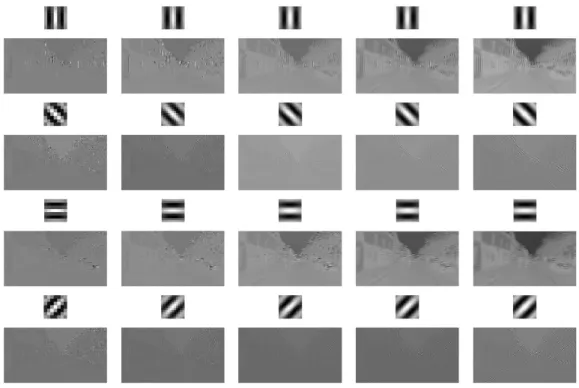
Where  corresponds to the spatial extent,  the orientation angle, and the frequency of the filter. In practice the spatial extent is often coupled with the frequency, and then a Gabor filter finally detects the presence of rectilinear periodic structures at a certain frequency and orientation. Gabor filters are acknowledged as a good model of one fundamental early visual function of the mammalians and then has been used in many object modelling and detection systems (Serre, Wolf, Bileschi, Riesenhuber, & Poggio, 2007). Figure 4 shows an example of direction/frequency decomposition using a bank of Gabor filters.

Figure 4: Local response to five scales and four orientations using a bank of Gabor filters.

Many real-time methods are based on collections of Haar filters (Viola & Jones, 2001), sort of approximations of derivative convolution kernels, which are particularly attractive for being computed very fast thanks using integral images. A Haar filter can be defined as a convolution kernel with rectangular support, with values only equal to -1 or +1. The number of operations needed to compute these filters do not depend on the size of the support, but on the number of rectangles with the same value inside the support. Figure 5 shows a few examples of Haar filters and their corresponding output.

Some methods radically differ from the previously cited ones in the sense that they begin by aggregating pixels in small homogeneous regions called “superpixels”, that will be used later as more reliable (and less numerous) individuals than pixels to extract relevant descriptors from images (Shotton, Winn, Rother, & Criminisi, 2007), (Micusik & Kosecka, 2009). In this

(11)

case, the lowest level operator is a segmentation algorithm, like the morphological watershed, which is fast enough and allows easy tuning of the size and relative contrast of the superpixels. Figure 6 shows examples of multi-level watershed superpixel segmentation. Like the contours, the superpixel approach can be better adapted than filter banks methods to the case of poorly textured objects.

(12)

(0) (1)

(2) (3)

Figure 6: An image (0) decomposed in superpixels by watershed (over)-segmentation of the morphological gradient image, with area closing of different sizes (1-3).

2 . 2

S ALI ENT POI NT AND RE GIONS

One important question rising in any method is whether the visual descriptors may be extracted from everywhere in the image or only from a few points or regions previously selected in the image. This can be interesting both to reduce the data flow and to improve the robustness (by selecting the most significant and stable structures), but it needs extra processing to perform the detection of salient structures. This detection generally uses a combination of filters and local detectors presented in the previous sub-section. A brief presentation of some significant detectors follows:

 The multiscale Harris detector (Mikolajczyk & Schmid, 2004) outputs the local maxima of an interest function computed from the autocorrelation matrix, estimated at various scales. It corresponds to corner points and it is rotation invariant (see Figure 7).

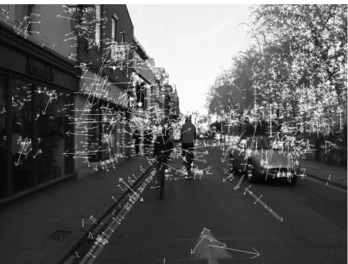
 The SIFT points (Lowe, 2004) are the local extrema, both in space and scale, of differences of Gaussian filters. They correspond to peak and valleys disappearing

(13)

during a progressive smoothing of the image. Every point is associated to a particular scale and orientation (see Figure 8)

 The SURF detector (Bay, Tuytelaars, & Van Gool, 2006) is a much faster multiscale detector which uses certain collection of Haar filters to approximate the multiscale second derivatives. The SURF salient points are then defined as the local maxima of the determinant of the Hessian matrix.

 The MSER detector (Matas, Chum, Urban, & Pajdla, 2002) uses a segmentation approach and selects superpixels with certain invariance and stability properties, corresponding to regional extrema of certain size, which are stable to perspective transformations.

 = 1.0  = 3.0  = 5.0

Figure 7: The Harris salient points (red crosses), calculated at three different scales.

Figure 8: The SIFT salient points. The salient point is located at the origin of the arrow; the length of the arrow represents the scale, its direction the argument of the gradient.

(14)

2 . 3

FE ATURE DESCRI PTORS AN D STATI STI CS

In this sub-section, we discuss the last part of visual representation, i.e. how the visual information is finally represented in the world model. The challenge of designing good descriptors is to find both concise and rich models, to be compared with the unknown objects from the video in an efficient and relevant way. The descriptor must capture essential structure, discard irrelevant details and lend itself to efficient metrics for comparison purposes.

When the image support is reduced to salient structures, the representation can be simply made by the collection of feature vectors corresponding to local structures calculated at every interest point location. For example, in (Schmid & Mohr, 1997), the descriptor attached to every Harris point (which is attached to a specific scale) is a vector made of Hilbert invariants (combinations of the local jet components with rotation invariance), calculated at the corresponding scale. This local approach has several advantages, like some robustness to deformation and occlusion, but it is very sensitive to the quantity and quality of detected salient points.

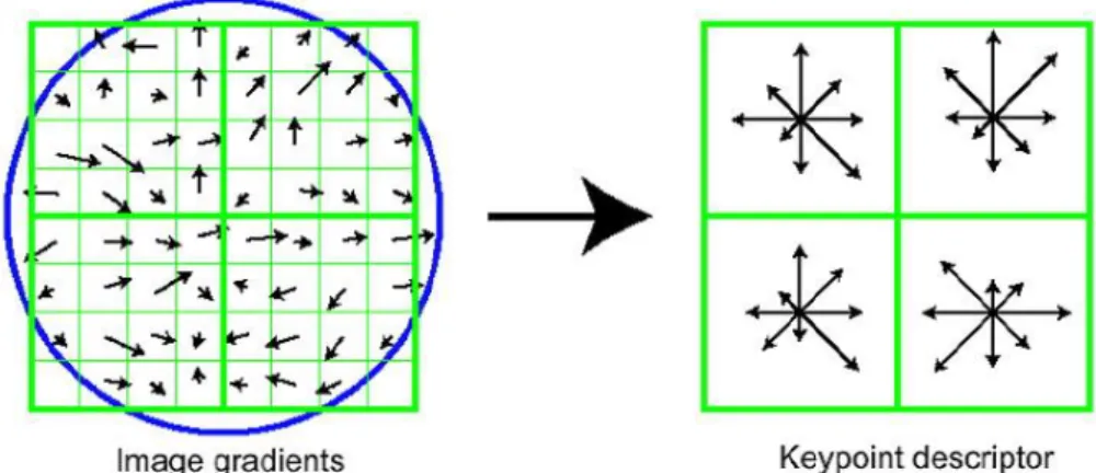
One common problem in designing descriptors is to find a good trade-off between local and global representation. Many approaches address this problem by computing spatial statistics or estimating regional tendency of a local measure. One of the most successful examples is the Histogram of Gradient orientations (HoG) and its variants. The descriptors usually attached to the SIFT (Lowe, 2004) or SURF (Bay, Tuytelaars, & Van Gool, 2006) salient points belong to this category. Every SIFT or SURF point is attached to the specific scale where it has been detected. It also comes with a specific orientation corresponding with the argument of the gradient calculated at the location point and the selected scale. Now the descriptors principle is to calculate the orientation of the gradients for every pixel around the salient point and to calculate the histogram of these orientations for one (or more) windows surrounding the salient point. The number of orientations is quantized to reduce the size of the descriptor, and the occurrence of every orientation is weighted in the histogram by (1) the distance of the pixel w.r.t. the salient point, and (2) the intensity of the gradient. Figure 9 and Figure 10 illustrate the actual descriptors proposed in the original articles.

Figure 9: SIFT descriptor, from (Lowe, 2004). The image is split in small blocks around the salient point, and the histogram of weighted and quantized orientation is calculated for each block. Dominant orientations correspond to the arrows of highest

(15)

Figure 10: One example of SURF descriptor, from (Bay, Tuytelaars, & Van Gool, 2006). The sum of some (absolute or signed) partial derivatives is recorded for small

sub-regions around the salient point in the image.

Histograms of orientations can also be used more densely, i.e. not only around salient points but in the whole image by dividing the image in (overlapping) blocks. In this case it is essential to use a dedicated orientation bin as “void” to code the homogeneous area without significant gradient. This is done in particular by (Hinterstoisser, Lepetit, Ilic, Fua, & Navab, 2010), who adopts a more radical approach (motivated by getting a very small code for real-time purposes), consisting in retaining only the dominant orientations present in a given block instead of a full histogram, turning the visual model into a simple binary code (see Figure 11).

Figure 11: Dominant orientations descriptor from (Hinterstoisser, Lepetit, Ilic, Fua, & Navab, 2010). The model records a subset of the (quantized) dominant orientations

present in a small image block. To measure the (binary) matching with the model (Figure), only one dominant orientation is calculated by block (blue arrows). One very popular class of methods in object modelling is the Bag-of-Features approach, which generalizes the concept of texton that has been used in texture recognition. The principle is based on the quantization of the n-dimensional descriptor space, which is then reduced to a codebook of N visual words (so called in analogy with the bag-of-words classification methods in linguistics). A visual class, object or image can then be represented by a histogram of visual words. A fundamental characteristic of these approaches is to mostly ignore the geometry of objects by considering only the presence of visual structures

(16)

and not the relations between them. However, taking into account more geometry can be done by considering higher order statistics, like co-occurrence between visual words.

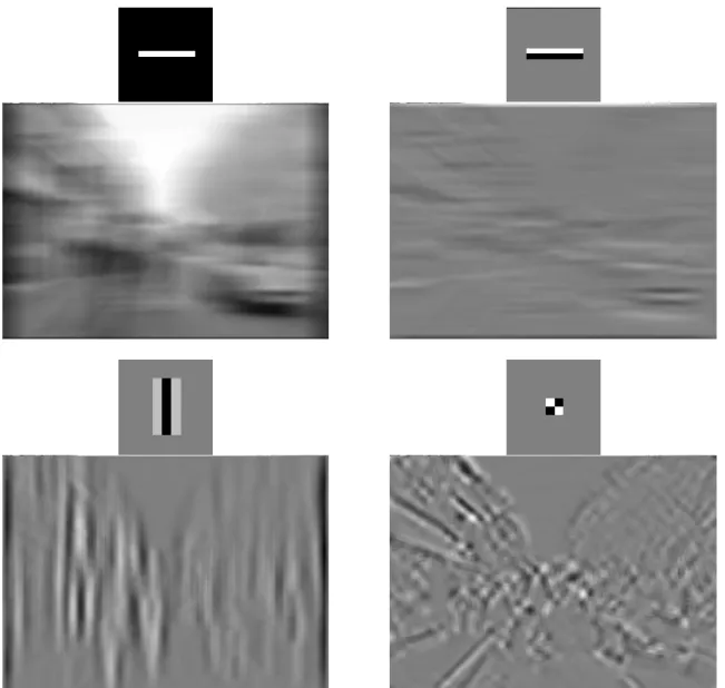
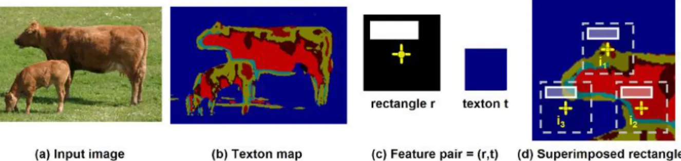
Bag-of-features (first order) classical approaches are known to work well for global image classification, e.g. place recognition, example based image retrieval, image categorization. But they are not designed to perform localization of the object in the image. To address this issue, several authors have proposed visual codebooks including information of relative localization. For example, (Murphy, Torralba, Eaton, & Freeman, 2006) use a codebook made of triplets (filter, patch, position). Every triplet is associated to a selected (learned) point and includes: (1) a filter from a filter bank, (2) the resulting patch containing the local output of the filter applied at the point location, and (3) the relative location of the point with respect to the object (See Figure 12). In (Shotton, Winn, Rother, & Criminisi, 2006), every code word or texton t is paired with a rectangular mask R made of an origin point and a rectangle. The matching measure at location x with the corresponding feature is obtained by counting the number of pixels of texton t within rectangle R when its origin is in x (See Figure 13).

Figure 12: Feature triplet from (Murphy, Torralba, Eaton, & Freeman, 2006), combining a filter f, a response patch P, and a relative localisation (blurred Dirac) g.

Figure 13: Texture shape by pairing texton index and relative location mask, according to (Shotton, Winn, Rother, & Criminisi, 2006)

(17)

3 .

LEARNING THE OBJECT MODEL

In this section we describe the techniques used to construct the world model from instances of objects captured off-line.

3 . 1

SELECTION OF THE OBJ ECT PROTOTYPES

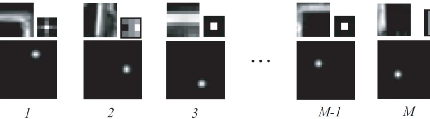
In the methods based on codebooks, object prototypes are constructed within a process of statistical reduction of the representation space. In this case the learning algorithm consists in summarizing the set of descriptors extracted from all the instances of objects captured in the learning base, to a (much smaller) set of significant vectors. The selection is usually performed by a vector clustering method such as K-means, but is sometimes done at random. Figure 14 shows some examples of the selected triplet prototypes used in (Murphy, Torralba, Eaton, & Freeman, 2006) to represent an object class.

Figure 14: Examples of the M triplet prototypes selected by vector quantization to represent the “Screen” object class in (Murphy, Torralba, Eaton, & Freeman, 2006)

(see also Figure 12).

In some cases the data reduction is done by reducing the dimensionality of the descriptor space, e.g. using principal component analysis or non-negative matrix factorization. In this case the object is not represented by prototypes, but by a small number of vectors from a new algebraic base representing the main directions of variation of the descriptor space.

3 . 2

FE ATURE SELECTION AN D LE ARNI NG

As previously explained, several techniques are based on the calculation of a large – potentially huge– number of operators from a bank of filters. However, only a small proportion of them are really significant for the detection of a certain class of objects. Automatically selecting the basic operators, and/or combining them to construct more sophisticated local detectors, is at the core of various object learning approaches.

One particularly successful technique is the Adaboost method applied for the selection and combination of the Haar filters (Viola & Jones, 2001). Although extremely fast to compute, the collection of all Haar filters computable within a region of reasonable size is much too high to be computable at detection time. The Adaboost algorithm learns the detection operators associated to a given class using a set of positive and negative example images. Every example is attributed a weight defining its influence in the learning process, the

(18)

weights being uniformly distributed at the beginning. Then, the algorithm iteratively selects the best “weak classifier” defined as the single Haar filter that best separate the positive and negative examples by simple threshold of its output. The best weak classifier is the one that minimizes the error measure obtained by summing all the weights of the failed examples. The weight of every example is then updated in such a way that the influence of the badly classified example increases in the selection of the next weak classifier, and so on. Finally a “strong classifier” is constructed using a linear combination of the weak classifiers, each weak classifier being weighted according to its single performance. See Figure 15 for the detailed algorithm.

Figure 15: Adaboost algorithm, taken from (Viola & Jones, 2001), for training one strong classifier using T weak classifiers. Every weak classifier is of the form

(19)

It is worth noting that Adaboost is an instance of more general boosting meta-algorithms, whose purpose is to automatically construct sophisticated classifiers from a set of simple (weak) binary classifiers. Boosting algorithms have been frequently used under different forms in object modelling and detection.

3 . 3

TEM PL ATE AN D SH APE H IERARCHI ES

As seen before, the most computationally efficient methods generally rely on rough descriptors (contours, dominant orientation), which are seriously affected by the shape variability in terms of size and point of view that can occur in the applications. One common way to address this problem is to construct, during the training phase, a higher level representation of the object combining different instances of descriptors of the same object appearing at different views. Those different instances should be organized in such a way to allow efficient matching during the detection phase. It generally corresponds to a hierarchical representation.

For example, in (Hinterstoisser, Lepetit, Ilic, Fua, & Navab, 2010), the authors starts with a collection of template vectors corresponding to block-wise dominant orientations captured from different views of a learned new object. The templates are grouped in clusters of similar templates, and every cluster can be assigned a generic descriptor vector (by simple OR operations), so that the template matching can be done efficiently using branch and bound in the detection phase.

In (Gavrila & Philomin, 1999), a coarse-to-fine contour hierarchy is constructed as a tree, every level of the tree being associated to a given resolution (the root represents the coarser resolution). At each level, the set of template contours at a given resolution is grouped in a few clusters; every cluster is associated to a node, and represented by a prototype, which is (ideally) the median contour of the cluster, i.e. the template contour minimizing its mean distance to other templates in the cluster. Clustering and choosing the prototypes is performed by minimizing an objective function using simulated annealing.

3 . 4

TR AI NI NG M ARKOV SUPE RPIXEL FIELDS

In the case of semantic segmentation, labelling is densely performed at the superpixel (region) level, and then the knowledge acquired from the training examples must be integrated in the priors of the superpixel classification method. Those methods are naturally well adapted to Markov Random Fields (MRF) based classification, where the topology of the MRF is given by the Region Adjacency Graph (RAG) of the segmentation, and potential functions defined on nodes and edges of the RAG are used as probabilistic modelling of the labelling decision, ruling (among others): the relation between a superpixel descriptor and its label, or the dependence between the labels of adjacent superpixels.

In this case, the learning phase corresponds to the training of the MRF and the construction of the potential functions. For example, in (Micusik & Kosecka, 2009), the potentials attached to higher order cliques are designed from the co-occurrence statistics of labels appearing in adjacent superpixels, obtained from the hand segmented training examples.

(20)

4 .

CONTEXT REPRES ENTATION

In many applications of object detection, taking the context into account in the modelling is very valuable, both in terms of robustness and computational efficiency. This is particularly true in the SPY project, where the camera will be embedded in a car, probably with a constant field of view. We are then dealing with street or road scenes, whose variability in terms of illumination and presence of objects can be large, but whose geometry and expected background (i.e. road, sky, building…) can be roughly predicted in a certain measure.

Such context representation involves global features of the image characterising the scene as a whole, but also some relations between the individual object models, in terms of temporal co-occurrence or spatial organization…

4 . 1

CONTEXT M ODELLI NG IN SEM ANTI C

SEGM ENTATI ON

The semantic segmentation methods necessarily include context modelling, because their purpose is to label every location (pixel or superpixel) of the scene, whether it belongs to an interest object or not. It is then natural to differentiate various background labels: sky, vegetation, road, etc. that turn out useful as context hints for the detection of the interest objects. As said earlier, those methods (Shotton, Winn, Rother, & Criminisi, 2007), (Micusik & Kosecka, 2009) use MRF formulations modelling conditional probabilities linking the values of labelling function , where S is the set of superpixels, and C the set of label classes. Let be the set of adjacent pairs of superpixels, such that (S,V) is the graph of adjacency of the segmentation. The semantic segmentation principle is to minimise an energy function E linking , S and V, for example:

∑

∑ ∑

Figure 16: Location conditional probability fields associated to different labels, used as contextual hints, taken from (Shotton, Winn, Rother, & Criminisi, 2007)

The first term relates to the visual appearance of superpixel s: sapp is the value of the visual descriptor calculated at s. The second term relates to the probability of co-occurrence of a couple of labels on adjacent pixels. This term can model the regularity (by attributing a higher probability to pairs with the same label) but also more contextual relationships like the likeliness of two labels to appear side by side, that can be learned from co-occurrence statistics (see Sec. 3.4). Finally the third term refers to the global context of the scene: sloc is the location (coordinates) of the superpixel, and the likeliness of a given label to appear at a given location in the image can also be learned from the training images. Figure 16 shows an example of the conditional probability fields learned from image bases for different labels. It is clear that those measures make sense and can be used in other framework than MRFs.

(21)

4 . 2

SCENE DESCRIPTORS

Sometimes the mere location hint discussed in the previous paragraph is not usable because the scene presents too much variability. This can occur in our application if the visual environment of the vehicle changes significantly, for example from a commercial urban street to a bare countryside road. In these cases, the “local” background must be estimated in order to exploit contextual information. This can be done by using global scene descriptors, calculated at run-time to improve the object detection and localisation.

Such descriptor is used by (Murphy, Torralba, Eaton, & Freeman, 2006), thanks to a global feature called “gist”. The gist of an image is obtained by (1) applying a bank of filters (e.g. Gabor) on the image to compute local responses in scale and orientation, (2) cutting the image in small blocks and calculating the average response for each scale and orientation and for every block, thus obtaining a vector of dimension , where n is the number of scales, m the number of orientations and p the number of blocks, (3) finally the dimension of the descriptor is reduced using Principal Component Analysis (PCA). Figure 17 illustrates the way the gist captures the global organisation of the textural features for two different scenes.

Figure 17: Illustration of the gist calculated for two images (top), taken from (Murphy, Torralba, Eaton, & Freeman, 2006). The bottom line shows two synthesis images with the same gist as the image above (obtained by iteratively modifying a random image) The gist is then used as a location prior in a similar manner as the previous subsection, except that the conditional probability for a label does not depend only on the coordinates of the pixel (or superpixel), but on the value of the gist at this location. Figure 18 shows an example where the value of the pixel is multiplied by the conditional probability for four different object labels. Now the conditional density of every label with respect to the gist needs to be learned with the other parameters of the world model, which is done in (Murphy, Torralba, Eaton, & Freeman, 2006) using multinomial regression and expectation minimisation (EM) algorithm.

(22)

Figure 18: Using the gist for location priming of four different object classes (screen, keyboard, car, pedestrian). Taken from (Murphy, Torralba, Eaton, & Freeman, 2006).

(23)

5 .

DETECTION AND LOC ALISATION

This section is dedicated to the online part of object detection systems, related to the tasks of detecting the presence of a known object and localise it in the image at run time. The evaluation of the computation cost is critical at this level, so we will particularly pay attention to the strategies that have been proposed to make this task as efficient as possible.

5 . 1

M ODEL M ATCH I NG M ETHO DS AND M E ASURES

Generally the first part of the detection task consists in applying to the image the same operators as those used in the object descriptors of the world model. Thus, in techniques where features have been selected (e.g. by boosting as in (Viola & Jones, 2001)), the detection consists in applying the selected filters and thresholds.

In semantic segmentation methods (Micusik & Kosecka, 2009), the detection/localisation task corresponds to the optimisation part of the MRF using for example Gibbs sampling, to calculate the label fields of minimal energy.

When the object model is made of a collection of local descriptors (Bay, Tuytelaars, & Van Gool, 2006) (Lowe, 2004) (Schmid & Mohr, 1997), the detection is performed by calculating the corresponding descriptor, either densely or only at salient point locations. The matching measure is then obtained by computing the distance between the descriptor vector vx calculated at pixel x, and every model descriptor vector vm, which can be simple Euclidean distance ( ) or Mahalanobis distance ( ₎ _{, where K is the covariance matrix of the descriptor distribution}

in the world model. When the learning is made off-line, K-1 is pre-calculated then the extra cost is negligible. Note that diagonalizing the covariance matrix is equivalent to performing a PCA (keeping all the dimensions). Once computed, point-wise classification can be done by nearest neighbour rule, while object localisation can be made by distance threshold followed by centroid calculation.

In some cases, the descriptor, or part of it, represents a distribution (e.g. histograms of colour), for which the direct bin-to-bin distance may perform poorly for comparison purposes, because of distortions due to quantization, light changes, or deformation, that can induce important shifts in the histogram domain. Many specific histogram distances have been proposed to address this problem; see for example (Pele & Werman, 2010).

In bio-mimetic detection systems, every pixel undergoes a sequence of local processing, grouping and matching inspired by the architecture of animal vision. Thus, in (Serre, Wolf, Bileschi, Riesenhuber, & Poggio, 2007), the detection task is performed in a feed-forward manner using two layers, each layer being the sequence of the application of simple cells (S) corresponding to local processing (filtering and matching), and complex cells (C) corresponding to max-pooling mechanisms. See Figure 19 for a graphical representation of the two-layer-four-stage systems.

(24)

Figure 19: Filtering layer (S1,C1) and matching layer (S2,C2) in the cortex-like object recognition system, taken from (Serre, Wolf, Bileschi, Riesenhuber, & Poggio, 2007). In the first (filtering) layer, the S1 stage corresponds to the application of the bank of filters (here Gabor filters). The C1 stage locally aggregates the output of filters by replacing every pixel value by the maximal value of the corresponding output over the neighbouring pixels and adjacent scales. The resolution at this stage may be reduced, and the scales regrouped in bands. This layer normally ignores the world model, unless feature selection is performed in the learning phase. In the second (matching) layer, the S2 stage corresponds to locally calculating difference between the output of C1 and a collection of template patches recorded in the learning phase. The C2 stage finally calculates the maximum of all S2 values for each template patch. Pixel level classification is obtained using the output of C2 through a simple linear classifier trained in the learning phase.

As reported in Section 2, some methods put particular efforts in the conciseness of the descriptor, for real-time purposes. A fortiori, special attention is dedicated to the efficiency of the runtime model matching tasks corresponding to their descriptors. In (Hinterstoisser, Lepetit, Ilic, Fua, & Navab, 2010), the image is cut in small blocks and dominant orientation is calculated for every block like in the model, except that one single dominant orientation (or none) is allowed for each block. If there is n possible orientations, every template block from the model (resp. every image block at the runtime detection), is coded with an n length binary word, whose possibly many (resp. only one or zero) bits have value 1. The template

(25)

matching is then calculated by a simple binary AND between the model and the image binary descriptor (See Figure 11 for an illustration of dominant orientation template matching). In the case of (Gavrila & Philomin, 1999), the object model is made of a hierarchy of template contours (see Section 3.3) whose best instances need to be found in the contour map of the current image at runtime. It is then necessary to compute very rapidly a matching measure between (small) contour prototypes and the current contour map at a particular location. This can be done very efficiently by computing distance transform of the current contour map, i.e. the function attributing to each pixel its distance to a contour pixel (see Figure 20 for an example), which are calculated very rapidly using constant time scanning procedures. The matching measure for a template contour at a given location x is then simply given by the sum of the distance transform along the template contour translated at position x.

Figure 20: Distance transform of the contour map of the current image for fast calculation of the matching measure with a template contour.

5 . 2

IM AGE EXPLOR ATI ON STR AT EGIES

To make the runtime detection/localisation task computationally tractable, it is necessary to reduce the number of operations performed on the current image whenever possible, by ignoring irrelevant parts of the image and concentrating on most promising regions. Mechanisms to rapidly decide whether a zone needs to be further explored or not are then highly desirable.

The first way of optimisation is to exploit the time redundancy and the motion coherence from one image to the other. In our context the scene geometry and the motion of the vehicle can be well modelled and estimated, so using the localisation information from the last frame is clearly valuable to improve the detection in the current frame. Generally those techniques relate to visual tracking, which is not detailed here. The time redundancy can also be addressed more specifically depending on the detection technique. For example, in semantic segmentation methods using MRF framework, overlapping superpixels from two consecutive frames can be linked by a temporal edge and attributed a particular energy term, e.g. ∑ (See Section 4.1).

Another important way to lower the computational cost is to perform partial work on a region in order to decide whether this region must be discarded or further investigated. This is frequently done in the object detection methods using cascaded computations. For example,

(26)

(Viola & Jones, 2001) apply a cascade of strong classifiers, constructed as follows. As seen in Section 3.2, Adaboost learning algorithm can be used to construct from a series of training examples a strong classifier, which is a combination of several (possibly many) weak classifiers (i.e. one Haar filter followed by a threshold). As a consequence, the best strong classifiers are very long to compute if they are calculated everywhere. The idea is then, instead of learning one single complex strong classifier, to learn first a very simple strong classifier (i.e. made of one or two weak classifiers), in such a way that the resulting classifier has maximal detection rate (and also high false detection rate), and to train a second – more complicated – strong classifier, using the false alarms of the previous one as the negative examples, and so on, until the desired performance is achieved. At the runtime level, the resulting sequence of classifiers is applied so that every classifier is applied on the image regions (windows) selected as possible object locations by the previous classifier. At its turn it rejects some regions and selects some other ones for further processing (See Figure 21).

Figure 21: Runtime application of a cascade of strong classifiers, according to (Viola & Jones, 2001).

Those motion based and content based image exploration mechanisms are highly desirable in a real-time context and should both be considered in our application.

(27)

6 .

BIBLIOGRAPHY

Bay, H., Tuytelaars, T., & Van Gool, L. (2006). SURF : Speeded Up Robust Features.

European Conference on Computer Vision.

Gavrila, D., & Philomin, V. (1999). Real-Time Object Detection for "Smart" Vehicles. ICCV (pp. 87-93). Kerkyra - Greece: IEEE.

Hinterstoisser, S., Lepetit, V., Ilic, S., Fua, P., & Navab, N. (2010). Dominant Orientation Templates for Real-Time Detection of Texture-Less Objects. CVPR. San Francisco, California (USA): IEEE.

Koenderink, J., & Van Doorn, A. (1987). Representation of local geometry in the visual system. Biological Cybernetics, 55, 367-375.

Lowe, D. (2004). Distinctive image features from scale-invariant key- points. Int. Journal of

Computer Vision, 60(2), 91-110.

Matas, J., Chum, O., Urban, M., & Pajdla, T. (2002). Robust wide-baseline stereo from maximally stable extremal regions. British Machine Vision Conference, (pp. 384-393). Cardiff.

Micusik, B., & Kosecka, J. (2009). Semantic Segmentation of Street Scenes by Superpixel Co-Occurrence and 3D Geometry. ICCV Workshop on Video-Oriented Object and

Event Classification. IEEE.

Mikolajczyk, K., & Schmid, C. (2004). Scale and Affine invariant interest point detectors. Int.

Journal of Computer Vision, 60(1), 63-86.

Murphy, K., Torralba, A., Eaton, D., & Freeman, W. (2006). Object detection and localization using local and global features. In Toward Category-Level Object Recognition (pp. 382-400). LNCS.

Pele, O., & Werman, M. (2010). The Quadratic-Chi Histogram Distance Family. ECCV. Schmid, C., & Mohr, R. (1997). Local grayvalue invariants for image retrieval. IEEE Trans. on

Pattern Analysis and Machine Intelligence, 19(5), 530-534.

Serre, T., Wolf, L., Bileschi, S., Riesenhuber, M., & Poggio, T. (2007). Robust Object Recognition with Coretx-Like Mechanisms. IEEE Trans. on Pattern Analysis and

Machine Intelligence, 411-426.

Shotton, J., Winn, J., Rother, C., & Criminisi, A. (2006). Textonboost: Joint appearance, shape and context modeling for multi-class object recognition and segmentation.

European Conference on Computer Vision (ECCV), (pp. 1-15).

Shotton, J., Winn, J., Rother, C., & Criminisi, A. (2007). TextonBoost for Image

Understanding: Multi-Class Object Recognition and Segmentation by Jointly Modeling Texture, Layout, and Context. Int. Journal of Computer Vision, 81(1), 2-23.

Viola, P., & Jones, M. (2001). Rapid Object Detection using a Boosted Cascade of Simple Features. CVPR (pp. 511-518). IEEE.

OBJECT MODELLING, DETECTION AND LOCALISATION IN MOBILE VIDEO: A STATE-OF-THE-ART

HAL Id: hal-01119691

https://hal.archives-ouvertes.fr/hal-01119691

OBJECT MODELLING, DETECTION AND

LOCALISATION IN MOBILE VIDEO: A

STATE-OF-THE-ART

Antoine Manzanera

To cite this version:

OBJECT MODELLING, DETECTION

AND LOCALISATION IN MOBILE

VIDEO: A STATE-OF-THE-ART

Antoine Manzanera

CONTENTS

ABSTRACT

1 .

SCOPE AND GENERAL AR CHITECTURE

1 . 1

I NTRODUCTION AND SCO PE

1 . 2

GENER AL ARC HITECTURE

2 .

OBJECT VISU AL REPRES ENTATION

2 . 1

FI LTER B ANKS AND LOC AL STRUCTURES

2 . 2

S ALI ENT POI NT AND RE GIONS

2 . 3

FE ATURE DESCRI PTORS AN D STATI STI CS

3 .

LEARNING THE OBJECT MODEL

3 . 1

SELECTION OF THE OBJ ECT PROTOTYPES

3 . 2

FE ATURE SELECTION AN D LE ARNI NG

3 . 3

TEM PL ATE AN D SH APE H IERARCHI ES

3 . 4

TR AI NI NG M ARKOV SUPE RPIXEL FIELDS

4 .

CONTEXT REPRES ENTATION

4 . 1

CONTEXT M ODELLI NG IN SEM ANTI C

SEGM ENTATI ON

4 . 2

SCENE DESCRIPTORS

5 .

DETECTION AND LOC ALISATION

5 . 1

M ODEL M ATCH I NG M ETHO DS AND M E ASURES

5 . 2

IM AGE EXPLOR ATI ON STR AT EGIES

6 .

BIBLIOGRAPHY