Publisher’s version / Version de l'éditeur:
Vous avez des questions? Nous pouvons vous aider. Pour communiquer directement avec un auteur, consultez la première page de la revue dans laquelle son article a été publié afin de trouver ses coordonnées. Si vous n’arrivez pas à les repérer, communiquez avec nous à [email protected].
Questions? Contact the NRC Publications Archive team at
[email protected]. If you wish to email the authors directly, please see the first page of the publication for their contact information.
https://publications-cnrc.canada.ca/fra/droits
L’accès à ce site Web et l’utilisation de son contenu sont assujettis aux conditions présentées dans le site LISEZ CES CONDITIONS ATTENTIVEMENT AVANT D’UTILISER CE SITE WEB.
Proceedings of the IASTED International Joint Conference on Artifical Intelligence
and Applications, 2003
READ THESE TERMS AND CONDITIONS CAREFULLY BEFORE USING THIS WEBSITE. https://nrc-publications.canada.ca/eng/copyright
NRC Publications Archive Record / Notice des Archives des publications du CNRC :
https://nrc-publications.canada.ca/eng/view/object/?id=945c1f15-4cf8-4e2d-b88f-09e4433a1168
https://publications-cnrc.canada.ca/fra/voir/objet/?id=945c1f15-4cf8-4e2d-b88f-09e4433a1168
NRC Publications Archive
Archives des publications du CNRC
This publication could be one of several versions: author’s original, accepted manuscript or the publisher’s version. / La version de cette publication peut être l’une des suivantes : la version prépublication de l’auteur, la version acceptée du manuscrit ou la version de l’éditeur.
Access and use of this website and the material on it are subject to the Terms and Conditions set forth at
Mining Multivariate Heterogeneous Time Series Models with
Computational Intelligence Techniques
National Research Council Canada Institute for Information Technology Conseil national de recherches Canada Institut de technologie de l'information
Mining Multivariate Heterogeneous Time
Series Models with Computational Intelligence
Techniques *
Valdés, J., and Barton, A.
September 2003
* published in Proceedings of the IASTED International Joint Conference on Artifical Intelligence and Applications. September 8-10, 2003, Benalmadena, Spain. ISBN: 0-88986-390-3, ISSN: 1482-7913, ACTA Press, Anaheim, USA, pp. 240-245. NRC 46513.
Copyright 2003 by
National Research Council of Canada
Permission is granted to quote short excerpts and to reproduce figures and tables from this report, provided that the source of such material is fully acknowledged.
Mining Multivariate Heterogeneous Time Series Models with
Computational Intelligence Techniques.
Julio J. Vald´es
National Research Council of Canada, Institute for Information Technology,
1200 Montreal Road, Ottawa ON K1A 0R6, Canada email: [email protected]
Alan J. Barton
National Research Council of Canada, Institute for Information Technology,
1200 Montreal Road, Ottawa ON K1A 0R6, Canada email: [email protected]
ABSTRACT
This paper presents experimental results of a computational intelligence algorithm for model discovery and data mining in heterogeneous, multivariate time series, possibly with missing values. It uses a hybrid neuro-fuzzy network with two different types of neurons trained with a non-traditional procedure. Models describing the multivariate time de-pendencies represent dependency patterns within the sig-nals and are encoded as binary strings representing neural networks (evolved using genetic algorithms). The present paper studies its properties from an experimental point of view focussing on: i) the influence of missing values, ii) the factors controlling the model search process, and iii) the effectiveness of the time series prediction results. Re-sults confirm that the algorithm i) possesses high tolerance to missing data, ii) has an error distribution skewed towards lower error values, iii) is capable of learning good models within large signal sets.
KEY WORDS
Neuro-fuzzy-genetic Architectures, Parallel Data Mining, Signal Processing, Neural Networks, Genetic Algorithms, Forecasting and Prediction
1 Introduction
Multivariate time series modelling and prediction is a very important subject because of the recent developments in sensor, communication and computer technologies, which allow the monitoring of complex processes in many do-mains (industry, environment, medicine, economics, etc.). It is especially important (in poorly known or altogether un-known complex processes) to discover patterns of delayed cause-effect dependencies. That is, to attempt to discover dependencies of one given target signal on past values of all signals (including itself) for particular time lags. This sit-uation becomes more complex when the multivariate time dependent process is composed of heterogeneous variables (numeric, non-numeric, fuzzy quantities and others), and when missing information is present. Finding models in this situation is a formidable task, given the large size of the search space and the complexity of the operations
in-volved. A soft-computing algorithm oriented to this kind of problem was developed elsewhere [9], as well as a par-allel implementation [10], using both a special kind of hy-brid neuro-fuzzy network and a genetic algorithm. This paper studies its properties in more depth from an experi-mental point of view, focussing on the influence of a broad range of missing values, the factors controlling the paral-lel computation, and on the effectiveness of the time series prediction results.
2 The Algorithm
The purpose is to discover dependency models in heteroge-neous, multivariate, time varying, complex processes from which observations with different degrees of completeness are obtained. A model expresses the relationship between values of a previously selected time series (the target), and a subset of the past values of the entire set of series. Hetero-geneity means both i) the presence of ratio, interval, ordinal or nominal scales, fuzzy and other magnitudes, and ii) the presence of different physical magnitudes contained within the signal set (e.g. temperatures, pressures, radiation lev-els, etc). The class of functional models considered by this algorithm is a generalized non-linear auto-regressive (AR) model (eq-1) (other functional models are also possible),
ST(t) =
F
S1(t − τ1,1), · · · , S1(t − τ1,p1), S2(t − τ2,1), · · · , S2(t − τ2,p2), . . . Sn(t − τn,1), · · · , Sn(t − τn,pn) (1)where ST(t)is the target signal at time t, Siis the i-th
time series, n is the total number of signals, piis the
num-ber of time lag terms from signal i influencing ST(t), τi,kis
the k-th lag term corresponding to signal i (k ∈ [1, pi]), and
F
is the unknown function describing the process. This ap-proach requires the simultaneous determination of: i) the number of required lags for each series, ii) the particular lags within each series carrying the dependency informa-tion, and iii) the prediction function. A requirement on functionF
is to minimize a suitable prediction error. This is approached with a soft computing procedure based on: (a)exploration of a subset of the model space with a genetic algorithm, and (b) use of a similarity-based neuro-fuzzy system representation for the unknown prediction function. Statistical or other classical approaches either have diffi-culties handling these kinds of situations or can not handle them at all [2] [7].
Evolving neuro-fuzzy networks with genetic algo-rithms has been explained in the literature for training
sin-gle networks [6], [3], [5]. Thus, the use of conventional
architectures and training procedures becomes prohibitive (due to the long waiting time for computations to com-plete). Other difficulties with classical approaches include
i) trying to find the number and composition of the
net-work hidden layers, ii) using mixed data types (numeric, non-numeric, fuzzy, etc), and iii) properly treating missing values. However, here the situation involves the construc-tion and evaluaconstruc-tion of thousands or millions of networks (i.e. because the network space is equivalent to the model space).
The search for models of the form given by eq-1 is performed with a genetic algorithm in conjunction with a neuro-fuzzy network. The dependency structure of the model is given by the collection of lags (delays) τi,k and
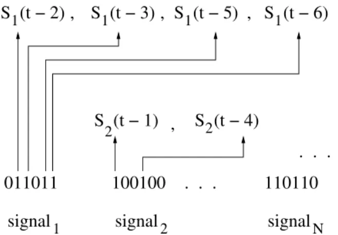
they are encoded as a binary string, which can be used as the chromosome representation by the genetic algorithm. Assuming that the dependencies are bounded by a max-imum lag value W for all N signals, a binary string of length N · W decoded as shown in Fig-1, accounts for a dependency model search space of size 2N ·W. Whereas,
the functional component (the function
F
in eq-1), needs to be found, inside a search space of infinite size. This is approached by using a neuro-fuzzy network which has gen-eral function approximation properties. The particular kind of network described below (based on heterogeneous neu-rons), fulfills this requirement and also has the advantage of having almost instantaneous training time in compari-son with classical neural networks. The present approach is based on the heterogeneous neuron model [8], [1], [11], which considers a neuron as a general mapping between heterogeneous multidimensional spaces h : ˆH × ˆH → Y, where Y is an abstract set. If ←−x , ←w ∈ ˆ− H (the input and the neuron weights respectively) and y ∈ Y, then y = h(←x , ←− w ).−In the similarity-based h-neuron model, the aggrega-tion funcaggrega-tion is given by a similarity funcaggrega-tion s(x, w) be-tween the input and the neuron weights (vectors from a het-erogeneous space), whereas the activation is a non-linear function. This neuron maps a n-dimensional heterogeneous space onto the extended [0,1] real interval. The output ex-presses the degree of similarity between the input pattern and the neuron weights s : ( ˆH× ˆH) → [0, 1]∪{X}, where X is the symbol denoting the missing value (Fig-2). A hybrid network layout using heterogeneous neurons in the hidden layer and classical neurons in the output layer is suitable for the purpose of model mining. For multivariate hetero-geneous time series, where a single time series is targeted for prediction, the network architecture is shown in (Fig-3).
1
S (t − 3)
2S (t − 4)
. . .
signal
2signal
1S (t − 6)
1 1S (t − 5)
. . .
Nsignal
S (t − 2)
1 2S (t − 1) ,
,
,
011011
100100
,
110110
Figure 1. Chromosome decoding for constructing a model based on eq-1 for the given set of signals.
During network operation each hidden layer neuron computes its similarity with the input vector and the k-best responses are retained (k is a pre-set number of h-neurons to select). They represent the fuzzy memberships of the in-puts w.r.t. the classes defined by their weights. Neurons in the output layer compute a normalized linear combination of the expected target values used as neuron weights (wi),
with the k-similarities coming from the hidden layer. output = (1/Θ)X i∈K hiwi, Θ = X i∈K hi (2)
where K is the set of k-best h-neurons of the hidden layer and hiis the similarity of the i-best h-neuron w.r.t the
in-put vector. The network outin-put is a fuzzy estimate of the predicted value. x
3.8
?
yellow ^F
nf
^no
O
^n
R
r
^n
N
n
H
^n
,
H
^n
{
{
{
{
h
(
(
Figure 2. A heterogeneous neuron with fuzzy, real (crisp), ordinal and nominal inputs.
Given a similarity function S and a target series the network is built and trained as follows: Set a similarity threshold T ∈ [0, 1] and extract the subset L of input pat-terns Ω (L ⊆ Ω) such that for every x ∈ Ω, there exist a l ∈ Lsuch that S(x, l) ≥ T . The elements of L will be the hidden layer h-neurons, while the output layer is built
H1 .. . Similarity Neuro−fuzzy Network H H 2 n O
Figure 3. A hybrid neuro-fuzzy network.
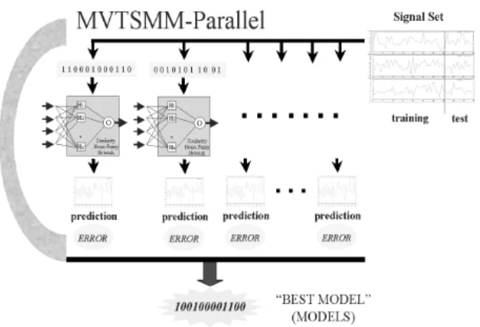
by using the corresponding target outputs as the weights of the neuron(s). This procedure is very fast and allows for the rapid construction and training of many networks. A dis-tributed parallel implementation following a master-worker (processor farming) approach was made. The system ar-chitecture of the parallel implementation of the algorithm is shown in Fig-4.
Figure 4. Multivariate Time Series Model Miner Sys-tem Architecture (MVTSMM). The arc is the parallel ge-netic algorithm evolving populations of similarity-based networks. They represent different dependency patterns which are generated by the master and evaluated by the workers during the search process.
3 Experimental setup
A multivariate time series data set consisting of 20 se-ries with 1140 observations of average monthly precipita-tion and temperatures from different sites in the Washing-ton State (USA) was chosen. They were recorded during the period 1895-1989 [4], and compiled by the National Oceanic and Atmospheric Administration (USA). Origi-nally, this data had no missing values and is shown in Fig-5. The precipitation signal for the West Olympic Coastal
drainage region (the top series) was chosen as the target for prediction. Contrary to the standard practice in time series analysis, no preprocessing was applied to the time series, in order to test the approximation capacity and robustness of the algorithm in the possibly worst conditions.
0 20 0 200 400 600 800 1000 1200 0 20 0 20 0 20 0 20 0 20 0 20 0 20 0 20 0 20 0 20 40 60 0 20 40 60 0 20 40 60 0 20 40 60 0 20 40 60 0 20 40 60 0 20 40 60 0 20 40 60 0 20 40 60 0 20 40 60 0 200 400 600 800 1000
Figure 5. Original data from Washington State observa-tion sites. (Upper 10 are Precipitaobserva-tion series and lower 10, Temperature series).
In addition to the original data, nine sets of time series were constructed by introducing into all 20 original series, 10%, 20%, · · · , up to 90% of uniformly distributed missing values. Missing values were introduced in a signal-wise manner. Each series was divided evenly into a training set and a test set. The training set for each signal contains the same percentage of introduced missing values, while the test sets were left intact. In this way, all signals contain exactly the same amount of missing values, as defined by the corresponding preset percentage.
transfor-mation (s = 1/(1 + d), where s is a similarity and d a dis-tance) of a modified Euclidean distance, accepting missing values. Given two vectors ←−x =< x
1, · · · , xn >, ←−y =<
y1, · · · , yn >∈ n, defined by a set of variables (i.e.
at-tributes) A = {A1, · · · , An}, let Ac ⊆ Abe the subset of
attributes s.t. xi 6= X and yi 6= X. The modified distance
function is de= (1/card(Ac))PAc(xi− yi)
2, which is a
normalized distance and therefore, independent of the num-ber of attributes. Consequently, no imputation of missing values to the data set is performed. That is, they are not replaced by any kind of estimate, but kept as gaps within the corresponding signals. The similarity threshold was set to 1, the number of responsive neurons in the hidden layer was varied in the range [3,11] by 2. The maximum lag depth was varied in the range [5,40] by 5, and the relative percentage of training/test fixed at 50%. For the genetic algorithm, the number of generations was fixed at 100 and the population size to 50. Binary chromosomes encoding model components as given by (equation 1 and Fig-1) were used with a double point crossover operator and standard bit-reversal mutation. Selection was kept constant (roulette wheel method) and complete population replacement with elitism were used. Crossover and mutation probabilities were 0.6 and 0.01 respectively.
Experiments were conceived to observe how Root Mean Squared Error (RMS error) was affected by several factors. Namely, i) the size of the maximum time lag from within which the dependencies will be searched (W ), ii) the number of best responsive neurons used in computing the predicted output estimate, and iii) the percentage of miss-ing values contained in the set (from 0 to 90%). A total of 400 experiments were made and from each, the 10 best models were retrieved, for a total of 4000 models investi-gated.
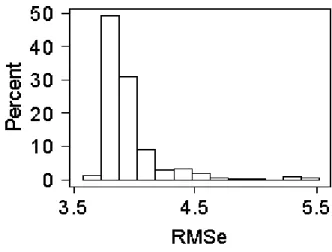
Figure 6. RMS Error distribution for all 4000 experiments The algorithm was run on a 17 unit cluster at the Institute of Biodiagnostics (National Research Council of Canada), composed by 4 dual Athlon processor units oper-ating at 1.666Ghz frequency, each with 2Gb RAM, 5 Xeon
Figure 7. Boxplots showing the main distribution features of the RMS Error for different percentages of missing val-ues, for all 4000 experiments.
processor units operating at 1.6Ghz with 1Gb RAM, 2 Pen-tium III units at 1Ghz with 256Mb RAM, 1 PenPen-tium III unit at 1Ghz with 512Mb RAM, 1 Pentium III unit at 930Mhz with 256Mb RAM, and 4 Pentium III units at 860Mhz with 512Mb RAM. This cluster uses Red Hat Linux 7.3, LAM/MPI 6.5.8 and has a shared network drive.
4 Results
The distribution of the 4000 RMS error values (Fig-6) is strongly skewed towards the lower end (Shapiro-Wilkes test rejected normality at 95%), indicating that the algo-rithm is less prone to give large prediction errors. The RMS error mean was 3.947535 and the bias and standard devia-tion of its sampling distribudevia-tion were estimated by boot-strapping to be 0.000136 and 0.004022 respectively. In practical terms, this means that the RMS error is an un-biased estimator.
The relations between the combination of percentage of missing values and the RMS Error are shown in Fig-7 as boxplots of their corresponding distributions.
The different percentages of missing values don’t ap-pear to exert a large influence on the RMS error for most of the missing value variants, with the exception of those greater than 70%. Overall, errors for all cases except these last ones, are within a relatively narrow band at the lower end for the Q1-Q3 interval. In the range [0% − 60%] there are no significantly different pairwise differences between error distributions. It is remarkable that even when 60% of the data is missing the ability of the algorithm in terms of discovering models capable of producing accurate predic-tions is not hindered. The algorithm isn’t affected until a large number of missing values are introduced into the data set, and even under such bad conditions, the rate of the de-grading effect is very low. Notice that a ninefold increase in percentage of missing data barely increases the RMS
Er-ror, as indicated by the comparison, for example, between the 90% and 10% cases. All of these features are indicative of very robust behavior.
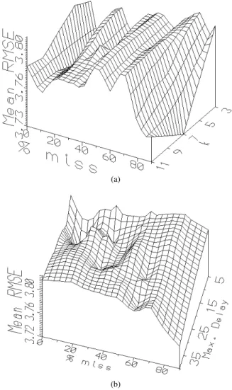
This skewed distribution is also an indication of the algorithm’s robustness, since in 90% of the experiments the time series were incomplete to some degree. The first quartile (Q1 = 3.8178) was chosen as an indicator of good error performance. The dependency of mean RMS errors with the number of responsive neurons (k) (controlling the fuzzy interpolation of equation-1), and the percentage of missing values is shown in (Fig-8(a)). In general, for a fixed amount of missing values the influence of this param-eter is not large. However, for complete or almost complete information, lower values of k (fewer terms in 1) have some advantage, whereas for high data shortages, larger values are required (i.e. fuzzy estimates with more terms) as could be expected.
(a)
(b)
Figure 8. (a) effect of % missing and k on RMSE, (b) effect of % missing and W on RMSE
In the case of 90% missing values, the behavior of the mean RMSE with the values of k differs substantially.
Figure 9. % of number of terms used in each signal for all lower range RMSE experiments
For k > 5 the errors drop, with a minimum at k = 7. Considering that this case corresponds to the largest per-cent of missing values, the situation is contradictory. How-ever, the error estimates are based on a very small number of samples (due to the extreme data dilution), hence their variances should be much higher, probably making the ob-served error differences non-significant (Fig-7). This situ-ation should be further investigated; nevertheless, the very fact that the algorithm is capable of providing useful results under such severe conditions indicates its high robustness and tolerance to ill-conditioned data.
In the case of the maximum lag depth (W) (Fig-8(b)), there is a decreasing trend for the errors as W increases for the whole range of missing values. Clearly, as data dilution increases, the algorithm is required to search deeper into the past in order to find meaningful dependencies from the point of view of effectively predicting the future values. It is interesting to note the local minima on the RMS er-ror surface are in almost perfect lineation, showing that for each percentage of missing values there is an optimum W (i.e. a defined search space), s.t. dependencies far beyond this lag, are probably meaningless or even noisy.
From the point of view of the composition of the 1001 discovered models in the lower error range, a rough pic-ture is given by the relative contribution of each signal to the model, measured by the number of terms (time lags) from the corresponding signal occurring in the model (Fig-9). It is interesting to see that the distribution is clearly multimodal, with some signals tending to contribute more frequently than others. Moreover, although the class of pre-cipitation signals (the first 10 in Fig-5) contributes the most (as could be expected, since the target is a precipitation sig-nal), there is an important contribution by the temperature signals, showing the physical relationship between precipi-tation and temperature. Sensitivity analysis are considered for future experiments.
5 Conclusions
The robustness of the algorithm has been shown by its dis-covery of models that have skewness towards lower error values, despite the large number of signals, their physi-cal heterogeneity and the (abnormally) large quantity of missing values. The algorithm was also capable of us-ing the 20 signals in a non-uniform way when predictus-ing the target signal. This shows the ability of this compu-tational intelligence-based technique for handling high di-mensional, time-varying data in an effective manner, with-out data preprocessing, and withwith-out imputation or assump-tions regarding the missing information. The method is ca-pable of intelligently assessing which are the most relevant signals w.r.t the target, as well as discovering the most in-teresting models and learning their composition in terms of the number and distribution of the significant lags. The experiments also revealed the most effective set of parame-ter values, for data mining applications for signal process-ing. These results are not generalizable until further ex-periments in other domains are conducted on larger, more complex data sets.
References
[1] Belanche, Ll. : Heterogeneous neural networks: The-ory and applications. PhD Thesis, Department of Lan-guages and Informatic Systems, Polytechnic Univer-sity of Catalonia, Barcelona, Spain, July,(2000). [2] Box, G., Jenkins, G. : Time Series Analysis,
Forecast-ing and Control. Holden-Day. (1976)
[3] Chen S.,Wu, Y., Luk, L. : Combined Genetic Algo-rithm Optimization and Regularized Orthogonal Least Squares Learning for Radial Basis Function Networks. IEEE-NN Trans. on Neural Networks, Vol 10, No. 5, pp-1239-1243, (1999)
[4] Masters,T. : Neural, Novel & Hybrid Algorithms for Time Series Prediction. John Wiley & Sons, (1995). [5] Maniezzo V. : Genetic evolution of the topology and
weight distribution of neural networks. IEEE Trans. on Neural Networks, Vol 5, pp-39-53, (1999)
[6] Montana D. Davis, L.: Training feedforward neural networks using genetic algorithms. Proceedings of the 11th International Joint Conference on Artificial In-telligence. Morgan Kaufman, California, pp. 762-767, 1989.
[7] Pole,A., West M., Harrison J. : Applied Bayesian Fore-casting and Time Series Analysis. Chapman & Hall, (1994).
[8] Vald´es,J.J. Garc´ıa, R. : A model for heterogeneous neurons and its use in configuring neural networks for classification problems. Proc. IWANN’97, Int. Conf.
On Artificial and Natural Neural Networks. Lecture Notes in Computer Science 1240, Springer Verlag,
(1997), pp.237-246..
[9] Vald´es,J.J. : Similarity-based Neuro-Fuzzy Networks and Genetic Algorithms in Time Series Models Dis-covery. NRC/ERB-1093, 9 pp. NRC 44919.(2002). [10] Vald´es,J.J., Mateescu, G. : Time Series Model
Min-ing with Similarity-Based Neuro-Fuzzy Networks and Genetic Algorithms: A Parallel Implementation. Third. Int. Conf. on Rough Sets and Current Trends in Com-puting RSCTC 2002. Malvern, PA, USA, Oct 14-17. Alpigini, Peters, Skowron, Zhong (Eds.) Lecture Notes in Computer Science (Lecture Notes in Artificial In-telligence Series) LNCS 2475, pp. 279-288. Springer-Verlag , 2002.
[11] Vald´es, J.J. : Similarity-based heterogeneous neurons in the context of general observational models. Neural