2-dimensional temperature modeling in Lower Granite Reservoir (Washington),

2-Dimensional Temperature Modeling in Lower Granite Reservoir

(Washington)

By

Yu-Im Loh

ENG

B.S. Civil and Environmental Engineering University of California at Berkeley, 1999

Submitted to the Department of Civil and Environmental Engineering in Partial Fulfillment of the Requirements for the degree of

Master of Engineering in Civil and Environmental Engineering At the

Massachusetts Institute of Technology

May 2000

@ 2000 Yu-Im Loh. All rights reserved.

The author hereby grants to MIT the permission to reproduce and to distribute publicly paper and electronic copies of this thesis document in whole or in part.

Signature of author:

Department of Civil and Environmental Engineering May 5, 2000 Certified by:

-77

Senior Research Engineer & Lecturer in Civil and Environmental Engineering Thesis Supervisor

Daniele Veneziano Chairman, Committee on Graduate Students

2-Dimensional Temperature Modeling in Lower Granite Reservoir (Washington)

BY

YU-IM LOH

Submitted to the Department of Civil and Environmental Engineering in Partial Fulfillment of the Requirements for the degree of Master of Engineering in Civil and Environmental Engineering

ABSTRACT

Lower Granite Reservoir is a 10-40 m deep riverine reservoir impounded by Lower Granite Dam. The reservoir displays vertical thermal stratification, especially in summer. A two-dimensional modeling tool, CE-QUAL-W2, was applied to the reservoir in current conditions. This model application simulated water surface temperatures at the forebay to within an average of 1 C of observed temperatures, but overpredicted stratification, so that the simulated temperatures at depth were about 10'C too low. Subsequently, the model was applied to hypothetical free-flowing conditions, that is, for the scenario in which all four dams in the reservoir have been removed for some time. The model predicted a slight decrease in water surface temperatures at the present location of Lower Granite Dam going from the with-dams to the no-dams scenario. The average difference for 1995 conditions was 0.4'C. Vertical stratification decreased in the no-dams scenario, with bottom temperatures increasing by about 1-4*C from the with-no-dams scenario. This is a possible undesirable effect of removing the dams. Water surface temperatures are the highest in the water column in the summer, when stratification occurs.

Thesis Supervisor: E. Eric Adams

Acknowledgments

I would like to express my thanks to my advisors Dr. Peter Shanahan and Dr. E. Eric Adams for

their invaluable advice and guidance.

To the people I have bothered with my e-mails and phone calls - Dave Reese of the United States Army Corps of Engineers, Charles C. Coutant of Oak Ridge National Laboratory, William A. Perkins and Marshall C. Richmond of Pacific Northwest National Laboratory, Scott Wells of Portland State University, and Ann Pembroke of Normandeau Associates - thank you for your unselfish help and interest.

Finally, thanks to my family and friends, especially my mother, Meng and my excellent suitemates.

Table of Contents

17

2.1

19

2.2 THEORY BEHIND THE MODEL

22

3.1 SOURCES

25

4.1 CALIBRATION 27 4.1.1 O utflow A djustm ent... 27

4.2 MODEL VERIFICATION 33 4.2.1 Vertical Temperature Profile ... 33

4.2.2 Water Surface Temperatures... 35

4.3 CONCLUSION 36 5.0 RESULTS... 37

5.1

37

REFERENCES ... 45

A PPENDIX B... 50

B.1 LOCATIONS 50

B.

1.1

B.1.2 Flow Gauge Stations ... 52

B. 1.3 Temperature M easurement Locations... 53

B.2 DATA 54

List of Figures

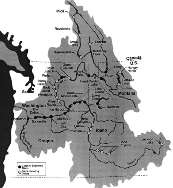
Figure 1.1 Map of Columbia River Basin and dams. Source: US Army Corps of Engineers. ... 9

Figure 1.2 Estimated Wild Sockeye passing the Uppermost Dam on the Snake River (Lower Granite Dam after 1974), 1962 to 1999 (May include Kokanee Prior to

1992). Source: USACE, 1999. ... 12

Figure 1.3 Water Surface Temperatures at the Forebay of Lower Granite Dam.

USACE Draft Lower Snake River Feasibility Study and Draft EIS, Appendix C,

1999 ... . . 13

Figure 1.4 Vertical Temperature Profile at various points along Lower Snake River (SNR-18: between Ice Harbor Dam and Lower Monumental Dam; SNR-1 08: Forebay, Lower Granite Dam; SNR-129, Lower Granite Reservoir), and just above Snake River-Clearwater River confluence (CW-1). USACE, 1999. 17 Figure 2.1 Truncated representation of Lower Snake River in CE-QUAL-W2. Layer

numbers are in the left-hand column while segment numbers are in the top row. Only segments 2 to 9 and layers 2 to 26 are represented here. Numbers in columns under each segment header are temperatures of respective cells, in degrees Celsius... 22

Figure 4.1 Forebay Elevations at Lower Granite Dam in 1993. Data Source: USACE,

2000... 29

Figure 4.2 Forebay Elevation in 1993 at Lower Granite Dam - Simulation 1 30 Figure 4.3 Simulated water surface elevations at the forebay of Lower Granite Dam,

1993. Inflows = outflows - evaporation loss of 1.4 m3_/s.31

Figure 4.4 Simulated forebay water surface temperatures in Lower Granite Reservoir,

1993. Inflows = outflows + evaporation loss of 1.4 m3/s.31

Figure 4.5 Comparison of simulated and observed water surface elevations at the forebay of Lower Granite Dam in 1993. Source of observed data: US Army Corps of Engineers, W alla W alla District... 32

Figure 4.6 Simulated and observed water surface temperatures at forebay, 1993, using the assumption that inflows = outflows. Source: US Army Corps of Engineers. ... 33

Figure 4.7 Vertical Temperature Profiles at Snake River Miles a) 129 (between Clearwater-Snake confluence and Lower Granite Dam), and, b) 108 (forebay, Lower Granite Dam). Observed data from Appendix C, USACE Draft EIS, 1999. ... . . 34

Figure 4.8 Simulated and observed water surface temperatures in Lower Granite Reservoir, 1995. Observed data from USACE...35

Figure 5.1 Water Surface temperatures simulated for the no-dams and with-dams scenarios. Conditions used were the same, as in the 1995 verification simulation. ... 3 9

Figure 5.2 Water surface elevations for the no-dams scenario. Conditions used were the same as in the 1995 verification simulation. ... 39

Figure 5.3 Vertical Temperature profiles at (a) RM 108 on August 10, and (b) RM 129 on August 13. Meteorological and inflow data as for 1995. Profiles are for

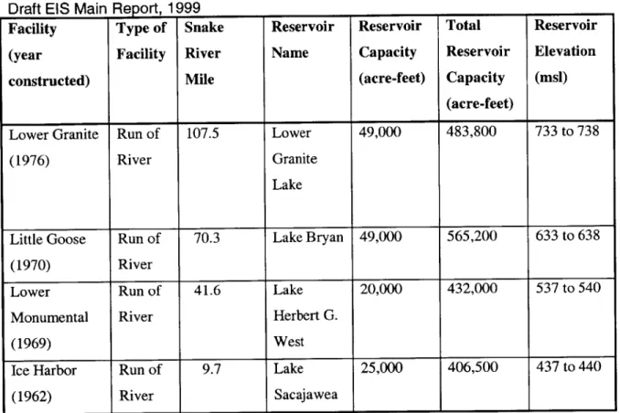
Table 1.1 Characteristics of the four Lower Snake River dams. Adapted from USACE Draft EIS Main Report, 1999 ... 11

Table 1.2 Frequency with which temperatures at the dams exceed 200C in unimpounded (free-flowing) conditions. Values were read off the graphs presented in the reports. (Data obtained from Yearsley, 1999; and from Perkins and Richmond, 1999.) ... . 16

1.0 Introduction

One of the most developed river systems in the world, the Columbia River system is home to several anadromous fish species, most of which are native to the region. As a tributary of the Columbia River system, the Snake River plays a major role in the life cycle of these fish species.

IsCo"p

1.1 History

Dams have been a part of the Columbia River Basin since the 1800s. The 20* century has seen tremendous development of the hydropower system on the Columbia River. Large projects such as Bonneville Dam and Grand Coulee Dam have served to change the hydrology of the river and the basin. Dams are not only meant to harness the river's energy for electric power, but also to enable navigation, flood control, and irrigation.

Hydropower development eventually spilled over to other rivers in the Northwest, albeit on a smaller scale. On the Lower Snake River, four dams were built over the course of 15 years, for much the same purposes as the Columbia River dams were constructed. The four dams that span the Lower Snake River are, from upriver to downriver, the Lower Granite, Little Goose, Lower Monumental, and Ice Harbor dams. Since the completion of the last of the four dams in 1975, they have been providing irrigation, navigation, and electricity generation capabilities to residents of the Northwest.

Table 1.1 Characteristics of the four

Main

Lower Snake River dams. Adapted from USACE

1.2 Effects of River Development on Anadromous Fish

The huge facilities constructed across the width of the Columbia and Lower Snake Rivers changed the hydrology and hydrodynamics of the rivers drastically. Shallow areas became flooded permanently, the river depth increased, and river velocity slowed.

The change in the rivers has far-reaching effects on the anadromous fish species in the river systems. These fish migrate to the Pacific Ocean from their spawning ground above the Snake River as juvenile smolts, and return 2 or more years later to spawn. The entire journey from the spawning ground to the ocean for anadromous fish in the Snake River carries them through 8 major dams, more if they start from above Dworshak Dam on Clearwater River.

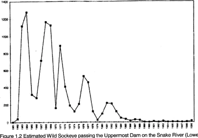
In 1991, the National Marine Fisheries Service listed the Snake River sockeye salmon as an endangered species. In 1992, spring and fall chinook salmon in the same river were listed as threatened species due to their rapid decline in recent decades (see Figure 1.2). In 1997, Snake

Facility Type of Snake Reservoir Reservoir Total Reservoir

(year Facility River Name Capacity Reservoir Elevation

constructed) Mile (acre-feet) Capacity (msl)

(acre-feet)

Lower Granite Run of 107.5 Lower 49,000 483,800 733 to 738

(1976) River Granite

Lake

Little Goose Run of 70.3 Lake Bryan 49,000 565,200 633 to 638

(1970) River

Lower Run of 41.6 Lake 20,000 432,000 537 to 540

Monumental River Herbert G.

(1969) West

Ice Harbor Run of 9.7 Lake 25,000 406,500 437 to 440

River steelhead joined the threatened species list (USACE, 1999). The population declines are manifested in lower numbers of returning adult fish migrating up the river system from the Pacific Ocean, and lower volumes of juveniles migrating down the river system toward the ocean.

Figure 1.2 Estimated Wild Sockeye passing the Uppermost Dam on the Snake River (Lower

Granite Dam after 1974), 1962 to 1999 (May include Kokanee Prior to 1992). Source:

USACE, 1999.

Several factors have been suggested as causes of the population decline. The most obvious cause of fish mortality is the obstruction of fish passage by the four dams on the Lower Snake River. Although ameliorative structures such as fish ladders for adult fish were installed when the dams were built, fish populations continue to decline as a result of poor passage rates through the dams. In recent years, the Corps has begun barging fish across dams in both the upstream and downstream directions. Facilities such as spillway deflectors improve water quality for fish that get "spilled" over the crest of the dam. Other fish passage measures have also been installed.

Apart from the direct fish mortality at the dams, it is suspected that the dams have indirectly caused population declines in the salmon and steelhead populations in a few different ways. Firstly, breeding habitats in the shallow areas of the natural river have been flooded to

create reservoirs. Secondly, the lower velocities in the river have probably decreased fish fitness

by increasing migration times. The decrease in robustness of the species is also attributed to the

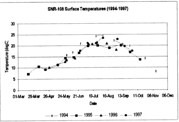
elevated temperatures in the river, which are far higher than optimal temperatures for successful reproduction and survival. Temperatures have reached maximums of 25'C in dry years, and

exceed the state's water quality standard of 20*C for most of the summer (see Figure 1.3).

-NR-18

-wF

- 19T5p

-

r

1994 9-7-1

-~ A

I

1-Mar 29-Mer

264*~ 24Ma

214uim

~I

*-Aug

13-Se

il-Oct 06-Nom

064)w

L_-_-

199

1996

*---Figure 1.3 Water Surface Temperatures at the Forebay of Lower Granite Dam. USACE

Draft Lower Snake River Feasibility Study and Draft EIS, Appendix C, 1999.

Other factors that are believed to contribute to the population declines are not related to the presence of the dams. These include changes in ocean conditions, which are known to cause dramatic declines in fish populations; global warming, which may have contributed to the elevated river temperatures to a not inconsiderable, although unquantified degree; and over-fishing, whether for recreation or industry.

that rely on the river system for their reproduction and survival. In response to a Biological Opinion released by the National Marine Fisheries Service in 1995, the Corps initiated a study of the Lower Snake River dams to determine how to improve fish passage on this stretch of the river system.

1.3 Proposed Solutions

In December 1999, the Corps released a feasibility study and draft Environmental Impact Statement describing the alternatives being considered to ameliorate the problems faced by anadromous fish in the Lower Snake River. The proposed alternatives follow.

A. "Existing Conditions"

Under this alternative, minor changes will be made to the current operating practices and facilities at the four dams. These changes are designed to decrease fish mortality rates in the passage through the Lower Snake River.

B. "Maximum Transport of Juvenile Salmon"

The operating principle behind this alternative is the minimization of in-river migration. Voluntary spills will not be used to promote migration. All fish collected at the dams will be transported by barge or truck to below Bonneville Dam. As spills will not be used to improve fish passage, spill deflectors and associated devices will not be installed for gas abatement.

C. "Major System Improvements"

Structural changes would be made to divert fish away from the turbines. The bulk of the improvements will occur on Lower Granite Dam. Surface bypass collectors will be installed at the dam. These collectors aim to guide most of the juvenile fish into smaller river volumes (i.e., near the water surface). The collected fish are then barged or trucked so that few juvenile fish will be left in the river below Lower Granite Dam.

D. "Dam Breaching"

The most drastic alternative of the four, dam breaching will involve removal of the earthen embankment portions of the four dams, effectively returning the Lower Snake to its natural river

levels. The drawdown behind the dams will be gradual (2 ft/day) in order to minimize structural failures of the river banks. The concrete sections and powerhouse structures will remain in the river, partly because the cost of removing them has no justifiable benefit, and partly to leave the

door open to the possibility of future power generation activities at the dams.

1A Project Motivation

While it is easy to measure fish mortality rates due to their having to negotiate a way through each dam, it is much harder to measure indirect effects that the dams have on fish. Few fish experts will dispute the claim that salmon in Lower Snake River suffer trauma that is a result of having their natural habitats changed. However, the mechanisms by which this trauma occurs, and the relative importance of each mechanism is a topic of much argument.

One characteristic of the river that is believed to have an impact on fish is the high water temperatures. Salmon species thrive at temperatures of 16-20*C. When temperatures exceed this

optimal range by even a few degrees, the reproductive processes are inhibited, fish fitness is decreased, and the population as a whole weakens.

Temperatures at the Snake River-Clearwater River confluence range from about 1 C to

20*C. Above this point, the flow is relatively fast. Below the confluence is the first of the four

artificial riverine reservoirs on the Lower Snake, Lower Granite Lake (called Lower Granite Reservoir in this paper). As the river proceeds downstream, temperatures naturally rise due to solar heating and higher ambient temperatures (since the flow goes from higher to lower

elevations). The construction of the dams has caused the river to widen and deepen by causing the flooding of previously exposed land. Thus, for the same inflow rate into the river, there is more surface area exposed to solar radiation. As a result, water entering the reservoirs behind the dams from upstream is heated up to a greater degree by the time it gets to the Columbia River.

If this last hypothesis that the four dams have caused the elevation of water temperatures

in the Lower Snake is proven correct, then the dams can be held responsible for the salmon decline on the premise that they are a cause of reduced fish fitness. The question to follow would be: What is to be done to lower temperatures in the Lower Snake River, assuming that lower temperatures would benefit the salmon population? Put in the context of the decision-making

process of the Corps: Would one or more of the proposed alternatives lower temperatures in the river, and if so, by how much?

1.5 Existing Temperature Models of the Lower Snake River

To find an answer to the latter question, the Corps modeled the Lower Snake River to see what temperatures would be in the scenario of a free-flowing river. At the same time, John Yearsley of the US Environmental Protection Agency also undertook to find the sources of the

elevated temperatures in the Lower Snake River.

A comparison of the conclusions derived from the two models reveals a disparity

between the returned results (see Table 1.2). These two models have been developed for use in the particular case of the Lower Snake River, and will probably feature prominently in a decision on whether to breach the dams.

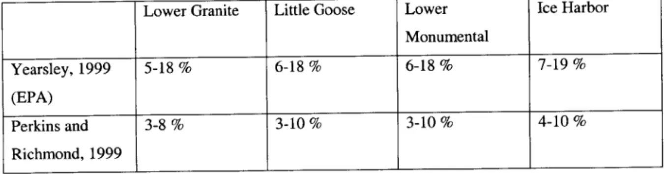
Table 1.2 Frequency with which temperatures at the dams exceed 200C in unimpounded

(free-flowing) conditions. Values were read off the graphs presented in the reports. (Data obtained from Yearsley, 1999; and from Perkins and Richmond, 1999.)

Lower Granite Little Goose Lower Ice Harbor

Monumental

Yearsley, 1999 5-18 % 6-18 % 6-18 % 7-19 %

(EPA)

Perkins and 3-8% 3-10% 3-10% 4-10%

Richmond, 1999

Both of these models are one-dimensional. In other words, they run on the assumption that the only significant variation in the temperature regime of the river is in the longitudinal

direction. Despite making the same basic assumption, the models return results that are significantly different. It bears mentioning that among the proposed alternatives, all will be costly, and some irreversible. An accurate assessment of the way each alternative will affect the temperature regime in the river is therefore vital to the decision-making process. Thus, the apparently small differences in the numbers presented by the two models may be significant.

1.6 Objective of Thesis

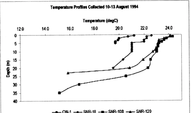
The Lower Snake River is not deep. Its depth at the upstream end is about 12 m; at the forebay of its most upstream dam, 32 m. In winter, when temperatures are cool, and in spring, when flows are high and fast, temperature across its depth is mostly uniform. However, when flows decrease in summer and ambient temperatures are high, vertical stratification may occur. Releases of cold water from Dworshak Dam (see Figure 1.1) in the summer would also encourage

stratification. This practice was started on a large scale in 1994 in order to augment flows in the Lower Snake River and thus decrease the average hydraulic residence time in summer (USACE,

1999). Dworshak Dam is a storage reservoir on the Clearwater River (upstream of lower Snake

River). The result is a vertical temperature variation, as shown in Figure 1.4.

Tempratr. Prailes COd 10-13 August 194

Tsfnpnrfuw (*VPC

120

140

WO,

180

200

22.0

X40

31

354

40.

CW1 -- SNIR48 -i- SNR-108 +- SNRA-129

Figure 1.4 Vertical Temperature Profile at various points along Lower Snake River (SNR-1 8: between Ice Harbor Dam and Lower Monumental Dam; SNR-1 08: Forebay, Lower Granite Dam; SNR-129, Lower Granite Reservoir), and just above Snake River-Clearwater River confluence (CW-1). USACE, 1999.

The presence of this variation raises the possibility that a 2-D temperature model may be more appropriate for the Lower Snake River than a 1-D model. The disagreement in the results of the two models applied to the river thus far may be partly due to the failure of the models to take

The objective of this thesis is to determine if there is sufficient basis to model the Lower Snake River as a two-dimensional water body. While it would be ideal to model the entire Snake River, the complexity of modeling a string of four reservoirs is too much to undertake in a preliminary study using the 2-D assumption. Effects of downstream reservoirs on the Columbia River would complicate the exercise. In any case, the goal is to find a basis, on conservative grounds, to model the Lower Snake River as a 2-D system. This is accomplished by modeling just one reservoir. Lower Granite Reservoir was picked because it has the least influence from the Columbia River Dams, and shows significant vertical stratification.

The Lower Granite Reservoir is the body of water that extends from just upstream of the Clearwater River-Snake River confluence to the Lower Granite dam. The dam is the most upstream of the four federal dams on the Lower Snake River. It was the last of the four to be constructed, having been completed in 1975, 14 years after Ice Harbor Dam came into service.

2.0 CE-QUAL-W2

Lower Granite Reservoir is a run-of-the-river reservoir, where the water elevation variability is about 1.5 m, from 223 m to 225 m over the space of a year. Run-of-the-river reservoirs earn their name from having a roughly constant water elevation. The depth of Lower Granite Reservoir varies from 10 m at the upstream end to 35 m at Lower Granite Dam. Its length is about 40 miles, while its width is only half a mile at the widest portion. These characteristics make it appropriate to assume river-like movement of water in the reservoir, meaning that water is not stagnant in most of the reservoir.

At any point along the reservoir's length, the meteorological conditions are assumed identical at every point across its width. As the main mode of heat exchange is through the water

surface, there is little variation in temperature across the relatively short width of the reservoir.

CE-QUAL-W2 was deemed to be the best available model for the purpose of modeling

temperature in Lower Granite Reservoir because it can represent the reservoir accurately in a simple model, has been used in several other applications, and is very well documented.

2.1 History and Applications

Derived from the Laterally Averaged Reservoir Model (LARM, see J.E. Edinger, 2000),

CE-QUAL-W2 is a "two-dimensional, laterally averaged, hydrodynamic and water quality

model" (Cole and Buchak, 1995). From the creation of the initial version in 1975, the model has been developed by several companies and government agencies to its current sophistication.

Among the government agencies that have used CE-QUAL-W2 are the US Geological Survey and the US Army Corps of Engineers. USGS used the model in their study of water movements in Shasta Lake (USGS, 2000). The simulation was for a year-long period in the lake from January to December. The Corps have used the model in several reservoir projects. Private firms which have employed the model are J.E. Edinger Associates, Inc. (J.E. Edinger, 2000), and Cornell University Utilities Department, which used it to determine the thermal characteristics of Lake Cayuga, NY (Cornell, 2000).

2.2 Theory behind the model

The theoretical basis of CE-QUAL-W2 has been extensively covered in other sources. The following is a summarized version of the User's Manual to Version 2.

The bases of CE-QUAL-W2 are laterally averaged momentum, continuity, and transport equations. The model can be used to model 21 constituents, and temperature. Factors that affect momentum such as salinity and temperature are built into the equations using an equation of state. Other influencing variables like local horizontal acceleration, momentum transfers in the

horizontal and vertical directions, horizontal pressure gradient, and vertical and horizontal shear stresses are also accounted for.

The first step in making a model of a river is to make a grid of the river volume. The volume is discretized into segments, which line up along the longitudinal axis of the river; and layers, which divide the river depth into horizontal volumes. Each cell therefore has a segment and layer number. For example, the coordinates (5, 7) would represent a cell in segment 7 and

layer 5. The variables associated with each cell center are width, density, constituent

concentration, and pressure; those associated with cell boundaries are horizontal and vertical velocities, and dispersion coefficients.

Simulations are carried out by solving six equations for six unknowns (see Appendix A). Inputs are inflows, outflows, and bathymetric data. The unknowns are free water surface

elevation, pressure, velocities in the horizontal and vertical directions, constituent concentrations, and density. The equations may be found in Appendix A, where an excerpt from the User Manual is included.

At each time-step, water surface elevation is first computed. This value is then used to compute horizontal velocity, which is consequently used to find vertical velocity from continuity. Constituent concentration is computed using the constituent balance equation. Finally, the vertical and horizontal velocities are used to solve for free water surface elevation, which is thus

The solution of the hydrodynamics of the system is the key to the simulations. Once this is done, the heat exchange algorithm is applied to compute temperatures based on surface heat exchange, and heat exchange between the water column and the sediments. Ice cover is also accounted for if the system in question undergoes any icing over.

Heat exchange through the water surface is calculated as follows:

Hn=Hs+Ha +He+Hc -(Hsr+Har+Hbr) (2-1)

Where

H n = the net rate of heat exchange across the water surface, W m -2 H , = incident short wave solar radiation, W m -2

H a = incident long wave radiation, W m -2

H e = reflected short wave solar radiation, W m -H c = reflected long wave radiation, W m

-H sr = back radiation from the water surface, W m

-H ar = evaporative heat loss, W m -H br = heat conduction, W m -2

The long wave atmospheric radiation is a function of air temperature and cloud cover (or vapor pressure) which are specified as time-varying series in the meteorology file. Short wave

solar radiation is either measured or computed from sun angle relationships and cloud cover. Evaporative heat loss is calculated from air temperature, dew point temperature, and surface

vapor pressure, which is calculated from the water surface temperature of each cell. Loss by conduction from the water surface is a function of the surface temperature. Back radiation is also a function of surface water temperature.

Sediment-water heat exchange is a function of the water temperature and the sediment temperature. The air temperature approximates sediment temperature. This is a rough assumption based on the idea that heat exchange at the water surface will far outweigh sediment-water heat exchange.

Returning to the hydrodynamics of the simulated system, density is an important factor that affects hydrodynamic computations. The code varies density according to temperature, salinity, and total solids content of each cell.

2.3 Application of CEQUAL-W2 to Lower Granite Reservoir

Lower Granite Reservoir is modeled as a single branch system consisting of 30 active segments and 27 active layers. Upstream and downstream boundary segments, segments 1 and 32 respectively, cap the two ends of the reservoir. These segments are inactive and have zero values for layer thicknesses. The active segments vary in length from 0

represent regions of the reservoir which vary considerably from orientation. Segments are oriented with respect to True North.

Layer 2 3 4 5 6 7 8 9 10 11 12 13 14 15 16 17 18 Depth 1.73 2.73 4.23 5.23 6.23 7.73 9.73 11.73 13.73 15.23 16.23 17.23 18.23 19.23 20.23 21.23 22.23 2 3.53 3.69 3.7 3.7 3.7 3.7 3.7 3.7 3.7 3 3.69 3.7 3.7 3.7 3.7 3.7 3.7 3.7 3.7 4 3.69 3.7 3.7 3.7 3.7 3.7 3.7 3.71 3.81

.25 to 1 mile. Short segments the adjacent segments in

5 3.69 3.7 3.7 3.7 3.7 3.7 3.7 3.7 3.7 3.7 6 3.69 3.7 3.7 3.7 3.7 3.7 3.7 3.7 3.7 3.7 3.7 3.7 3.7 7 3.69 3.7 3.7 3.7 3.7 3.7 3.7 3.7 3.7 3.7 3.7 3.7 3.7 3.7 3.7 3.7

Figure 2.1 Truncated representation of Lower Snake River in CE-QUAL-W2. Layer numbers

are in the left-hand column while segment numbers are in the top row. Only segments 2 to 8

and layers 2 to 26 are represented here. Numbers in columns under each segment header

are temperatures of respective cells, in degrees Celsius.

In active segments, some or all of the layers are utilized, with active layers given a thickness of 1 or 2 m, and inactive layers given a thickness of zero. There are also two boundary layers, one on top and at least one on the bottom at all times. These layers are given a thickness of

1 m. The thickness of 1 or 2 m was chosen based on Figure 1.4, as significant temperature

variation occurs over changes of water depth of the order of 1 m. The placement of 1 and 2-m

8 3.69 3.7 3.7 3.7 3.7 3.7 3.7 3.7 3.7 3.7 3.7 3.7 3.7 3.7

layers within the water column is loosely based on the observed vertical temperature profile in the summer of 1994, as this time of year represents the worst-case scenario for reservoir

stratification, when flows are low and solar heating is at its greatest.

Time-varying inputs required for a simulation of temperatures over time and space are inflows to the reservoir, inflow temperatures, and meteorological conditions over the reservoir. Inflows are daily average values from both the Snake River just above the Clearwater-Snake confluence, and the Clearwater River into the Lower Snake. These flows are assumed to be similar to those recorded at the Snake River near Anatone, WA; and at Spalding, ID on the Clearwater River. Streamflow data was obtained from the USGS website (USGS Water, 2000).

Inflow temperatures from these two sources are also daily average water temperatures. The temperatures of these flows were approximated by data collected at the Snake River near Anatone for the Snake River inflow, and by temperatures at Orofino (Clearwater River Mile 44.6), adjusted for the summer months. Orofino was picked because it is the closest reliable

station on the Clearwater River with year-round daily temperature data. The Orofino data was adjusted downward by 1-5'C for the summer months (June 19 - Aug 21 in 1993) to compensate for the colder temperatures of the Dworshak Dam releases into the Lower Snake in summer. These new temperatures were compared to daily average temperatures based on temperatures collected hourly 1.5 river miles downstream of Dworshak Dam tailrace (which were only available for Aug - September in 1993, and April - September in 1994, 1995 and 1996). In general, the adjusted temperatures gave good agreement with Dworshak Dam tailrace temperatures. Wherever possible, temperatures at Dworshak Dam tailrace were used as approximations of Clearwater tributary inflow temperatures. For instance, in 1995, Orofino temperatures were used until April 24, Dworshak Dam tailrace from April 25-Sept 30, with adjusted Orofino temperatures for Sept 12-13, and for 15 days after the Dworshak Dam data stops. See Appendix B for temperature data at Orofino and 1.5 Miles downstream of Dworshak Dam tailrace. Temperature data was obtained from the Streamnet web-site (Streamnet, 2000).

Meteorology at Lower Granite Reservoir was approximated by data collected at Lewiston Nez Perce County Airport. Data were either found as daily averages or calculated from hourly

observations to give daily averages. Five measurements define the meteorology of the region in this model: air temperature, dew point, wind speed and direction, and cloud cover.

Note that all data used is presented in Appendix B together with descriptions of the data collection stations.

In order to model Lower Granite Reservoir to an accuracy of a day without requiring excessive computing power or run-time, daily inputs were preferred over hourly inputs. This chapter summarizes the sources of the data used in the calibration, verification, and, indirectly, in the simulation phases, and describes how data was organized into input file format. The final section discusses the quality of data used, and what was done when poor quality data was encountered.

3.1 Sources

Temperature data for inflows was obtained from files on the website of Streamnet (Streamnet, 2000). Most of this data was obtained from the US Army Corps of Engineers at Walla Walla District. Flows into Lower Granite from Snake River and Clearwater River were obtained from the USGS water data web-site (USGS, 2000). Meteorological data came from the records of the US Geological Survey. Finally, bathymetry of Lower Granite Reservoir was approximated from soundings mapped in Nautical Chart 18547 produced by the National Oceanic and Atmospheric Administration (NOAA, 1993).

3.2 Data Organization

In general, data from the various sources was in an easy-to-use format. Adjustments that were made were usually simple addition and subtraction operations.

Bathymetry was determined by using depth soundings indicated on the Nautical Chart

18547 (NOAA, 1993) to draw simple reservoir cross-sections in Microsoft Excel. Cross sections

were taken at variable intervals along the length of the reservoir. These intervals ranged from 400 m to 4300 m, depending on the curvature and, hence, variability of the cross section. Reservoir stretches with large curvature were divided into shorter intervals while relatively straight stretches were assumed to have the same cross-section over long distances. See Appendix C for

bathymetric cross-sections used. The Clearwater River tributary was not modeled as a section, but rather as a simple inflow into the third active upstream segment of the main branch.

Water temperatures for the main branch are assumed to be those measured on the Snake River near Anatone. Tributary temperatures are assumed to be the temperature observed at

Orofino for pre-and-post summer months, and the flow-weighted average of temperatures measured at Dworshak Dam tailrace and at Orofino for the period every year when Dworshak Dam tailrace temperatures were recorded (mid or late April to September for 1994 and 1995). The measurements are daily average temperatures based on hourly gauge measurements.

Inflows were assumed to come from the Snake River above the Clearwater-Snake confluence and from the Clearwater River. The Snake River inflow was taken to be that near Anatone, where flows are measured at Station 13334300. Clearwater inflows were taken to be that measured at Spalding, ID (Station 13342500), a location downstream of Orofino and Dworshak Dam, about 10 miles upstream of the Clearwater-Snake confluence. The Clearwater inflow was modeled as a point tributary inflow into segment 4 of the main branch (note that the

upstream boundary segment is Segment 1 and is inactive), while the Snake River inflow was equally divided over the entire cross-section (i.e., single-temperature inflow).

Outflows were assumed to occur only at the dam. These outflows were mainly through the turbines, which occupy the southern third of the dam's length. In May and June of every year, however, additional water is spilled over the crest of the dam. For these periods, spills and generator outflow together constitute the outflow value. Evaporation is the other means by which water is lost from the reservoir and is modeled by the software.

Meteorological data was mostly obtained as daily measurements and is used as such. The exception is daily average wind direction, which was obtained by taking the average of the hourly wind direction measurements, weighted by the corresponding hourly wind speeds. The

measurement of wind direction and speed was only done for daylight hours.

3.3 Data Quality

All of the data used comes from reputable sources and appears reasonable. As far as

possible, data was checked either directly with similar data from other sources (e.g., flow at one location compared to flows at other nearby locations) or indirectly with data from the same time periods in other years. For instance, flows from different years were compared to identify obvious erroneous data entries.

4.0 Model Calibration and Verification

This section describes the process by which CE-QUAL-W2 was calibrated for the Lower Granite Reservoir system. Calibration was based on the year 1993. Subsequently, the model was verified using the years 1994 and 1995 to encompass a range of weather conditions. 1994 was a dry year, with flows ranging from 10 to 75 kcfs; 1995 had mean monthly flows close to historical averages for the first half of the year, and slightly higher flows for the rest of the year. Unusually wet years are not modeled because they represent the least critical condition for Lower Snake salmon species.

4.1 Calibration

Calibration is the process by which a model is adjusted to give the most realistic

simulation results. In the case of CE-QUAL-W2 for Lower Granite Reservoir, input outflows had to be varied somewhat from the Corps' data in order for the simulation to be in good agreement with the observed data. Good agreement means similar water surface temperatures, vertical temperature profiles, and water elevations. Note that not all of the inflows and outflows of the system were known. Thus, while all major flows were represented, it is possible that flows into or out of the reservoir between the Clearwater-Snake confluence and the Lower Granite Dam that were not represented in this model could have had an impact on the simulation. It is in

anticipation of such inaccuracies in data input that outflows at the dam were adjusted. These adjustments are described below.

4.1.1 Outflow Adjustment

Lower Granite Dam has several functions. The reservoir is used for navigation, hydropower generation, recreation, and "incidental irrigation" (USACE, 2000). Hydropower

generation is served by any non-spilled release of water from the upstream to the downstream side of the dam. Having the reservoir for navigation means that the height of the dam is limited to allow for the operation of locks. This means the dam cannot perform other storage functions, or can only fulfil them to a limited degree as a secondary purpose.

Recreation generally involves maintaining a full reservoir to allow for activities such as boating, swimming, fishing, and water sports. Excessive drawdown usually creates undesirable conditions for recreation. For instance, benthic surfaces may be exposed and become foul smelling areas. Boat piers may also be too far above the water surface to be functional. Despite these considerations, recreational function is usually incidental to other purposes of the reservoir.

Irrigation is a secondary purpose of creating the backwater that is Lower Granite Reservoir. As mentioned on the Corps' website, irrigation needs served by the reservoir are incidental and not sufficient to account for large sudden withdrawals from the reservoir. The fluctuation of water surface elevation over the course of a year is due mainly to the purposeful release of water from the reservoir to augment downstream flows for navigation. This occurs in the dry season when flows are low downstream due to lack of precipitation and higher rates of evaporation brought about by higher water temperatures and drier ambient air.

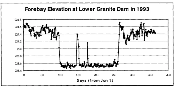
The pattern seen in Figure 4.1 shows a sharp drop in water elevation from 224.45 m to

223.6 m over just 4 days. The resulting elevation is maintained for several months (with small

peaks due to storm events) until the winter months, when the elevation is increased back to the January elevation, just as suddenly as it was decreased. This is typical dam operation for

navigation purposes and for flood control. In winter and spring, the main source of river flow will be stormwater. In the summer, precipitation halts and snowmelt becomes the main source. In

order to prevent flooding of the surrounding lands as well as to provide navigation flows downstream, the elevation in the reservoir is kept at a minimum operating level (minimum to maintain recreational activities). In these same four days, however, flows recorded by the Corps are not especially high (USACE, 2000). This is unusual because typical practice is to release excess water over the crest of the dam or to run it through the hydropower turbines. Thus, higher rates of outflow from the reservoir than those shown on the Corps' datasheets are expected. The total outflow data on the web-site is possibly erroneous.

Initially, outflows were put into the model as single average daily outflows. These values came directly from the Corps' ftp website for the Northwestern Division (USACE, 2000). When the program was run, the water surface elevation increased throughout the year, reaching

elevations about 20 m higher than the maximum water surface elevation at the forebay. Figure 4.1 indicates the observed water surface elevations in 1993 that are distinctly different from this initial prediction.

Forebay Elevation at Lower Granite Dam in 1993

Days (from Jan 1)

Figure 4.1 Forebay Elevations at Lower Granite Dam in 1993. Data Source: USACE, 2000.

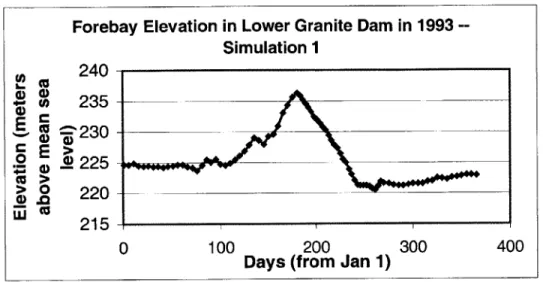
The root of the increasing elevations seemed to be unaccounted outflows from the reservoir. To address this problem, the volume of water "accumulated" in the reservoir by the end of the year was divided unequally among the 365 daily outflows for the year. The unequal

division was meant to represent irrigation withdrawals from the reservoir that were not

represented in the outflow at the dam. Due to lack of knowledge regarding the locations, volumes and timing of the withdrawals, the withdrawals were approximated by adding volumes to the outflow at the dam. As irrigation withdrawals are expected to be low in winter and spring, and higher in summer and fall, the accumulated volume from the initial run was divided to reflect this condition. For instance, the first run using this condition used outflows that were 20 m3_{/s higher}

from January to March, 50 m3/s from April to June, 129 m3/s from July to August, 50 m3_{/s in}

September, and 20 m3_{/s from October to December. The results of this run in terms of water}

4 U)

eE

>

Wa >

> 0

Forebay Elevation in Lower Granite Dam in 1993

--Simulation 1

240

235

230

225

220

215

400

100

200

Days (from Jan 1)

Figure 4.2 Forebay Elevation in 1993 at Lower Granite Dam - Simulation 1

This method of guessing additional outflows for different times of the year was unsuccessful in reproducing the observed water surface elevations. A new method was thus devised based on the following assumptions:

1. There are processes besides inflow and outflow by which the water balance in the reservoir is

affected. Processes that decrease the water volume are irrigation withdrawals and evaporation. Conversely, precipitation and inflow from tributaries or runoff between the Snake-Clearwater confluence and Lower Granite dam cause an increase in the water volume. 2. Precipitation is roughly equal to evaporation for the year.

3. Evaporation data from NOAA (NOAA, 1983) indicates that the mean rate of evaporation for

the lakes in the Lewiston region from 1946 to 1955 is about 40 in./year. This works out to about 1 m3/s. As the "excess" volume in the reservoir is equivalent to 46.6 m3/s, and

evaporation accounts for just 1 m3/s, the bulk of the excess volume must be due to unknown quantities such as irrigation withdrawals or due to erroneous flow data. As these are not known, the simple assumption that inflows are equal to outflows (less evaporation loss) is made. Inflows are equal to outflows for the same day, as the reservoir is run-of-the-river (i.e., elevation does not change much).

Figures 4.3 and 4.4 show the results of a simulation done with outflows set equal to inflows minus evaporation loss. Observed temperature data is superimposed for comparison.

Water Surface Elevations at Forebay (Lower

Granite Dam) -- Simulated, 1993 ( outflows

=

inflows - evap. loss)

225.6

a)W

225.4-o

o

*225

-225

S224.8-224.6

0

100

200

300

400

Days from Jan 1

Figure 4.3 Simulated water surface elevations at the forebay of Lower Granite Dam, 1993.

Inflows

outflows

evaporation loss of 1.4

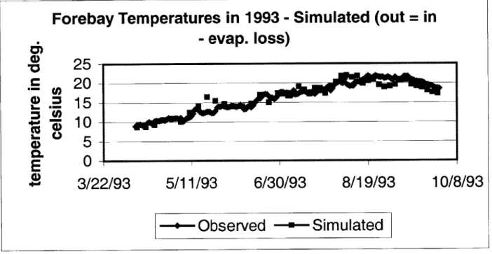
Forebay Temperatures in 1993 - Simulated (out = in

-

evap. loss)

*a

E

10/8/93

8/19/93

6/30/93

2/93

(I)

U

25

20

15

10

5

0

3/2

-+-Observed ---

Simulated

Figure 4.4 Simulated forebay water surface temperatures in Lower Granite Reservoir, 1993.

Inflows = outflows + evaporation loss of 1.4 m

_/s.

The increase in elevation over the year in the latter simulation led to the inference that outflow was insufficient in the model. Thus, the evaporation loss was omitted from outflows, and outflows were set equal to inflows. The following figure shows the simulated and observed elevations. Note that inflows are the same in both simulations. Outflows are either equal to these

5/11/93

-f9e*~.

From the figure, it is clear that subtracting a constant volume from each day's outflows has the effect of increasing water elevations to higher than observed values. If outflows are set equal to inflows, there is a decrease in elevation throughout the year. The simulated elevation at the end of the year deviates by the same amount from the observed end-year value. The inference is that a smaller net constant decrease in daily outflow values will allow better replication of observed elevations (although not to the extent of reproducing sharp drops and rises in elevation). The aim here is to maintain a somewhat constant elevation, such that the elevation at the end of the year is roughly the same as at the beginning of the year.

Water Surface Elevations-Simulated vs. Observed 0225.5

M2

-Cc 223.5

-223 i ,

0

100

200

300

400

days from Jan 1, 1993

- in = out --- in = out + evaporation loss --- observed

Figure 4.5 Comparison of simulated and observed water surface elevations at the forebay of Lower Granite Dam in 1993. Source of observed data: US Army Corps of Engineers, Walla Walla District.

The problem with adjusting outflows in order to obtain a constant elevation is that these adjustments might change with changes in annual conditions. In this case, the simplest

assumption that the reservoir is run-of-the-river is the best, because this assumption holds for all years. The simulation results obtained for water surface elevation with this assumption show variations that are within the observed elevation variation, that is, within the 223.5 m - 224.7 m range. Without a rough knowledge of the sources and sinks of flow in the reservoir, setting inflows to outflows is the best calibration option for this run-of-the-river reservoir.

The temperature-time plot for the simulation where inflows are equal to outflows gives good agreement with observed temperatures. The temperatures compared are at the surface of the forebay of the dam. Observed data were obtained from the Streamnet website (Streamnet, 2000).

Water Surface Temperatures at forebay, 1993

25 2015 S10 -a. E 0 1 3/22/93 5/11/93 6/30/93 8/19/93 10/8/93 --- Observed w Simulated

Figure 4.6 Simulated and observed water surface temperatures at forebay, 1993, using the assumption that inflows = outflows. Source: US Army Corps of Engineers.

Given the uncertainties in sources and sinks to the reservoir, the simulation is relatively accurate in its reproduction of forebay temperatures in 1993. The average absolute difference is about 1*C, while the simulated temperatures exceed observed temperatures by 0.20C. The maximum difference was 4.2*C (the simulated temperature exceeded the observed temperature).

4.2 Model Verification

The model was verified on two counts. Firstly, it was verified with respect to vertical temperature profile, for which observed data is available for 1994. Secondly, the water surface temperatures simulated were compared to observed data for a year with average flows, 1995. The procedure for simulation is as described for model calibration.

4.2.1 Vertical Temperature Profile

As only two observed data sets are available (both from 1994), there is insufficient information with which to calibrate the model to simulate correct vertical temperature profiles. Only 1994 vertical temperature data was available. As 1994 was a low-flow, and, therefore,

verification. Thus, vertical temperature profiles generated by the software should be treated with caution and only used in relative comparisons (i.e., comparisons between different simulated years) and to make qualitative inferences only.

Figure 4.7 shows simulated and observed vertical temperature profiles at two locations along Lower Snake River, both of which lie within Lower Granite Reservoir. The simulation overestimates stratification in both locations. The discrepancy is possibly due to cold water influxes from Clearwater River, which have adjusted temperatures (see Chapter 3) that are too low. The more likely reason is that the model fails to account for mixing between the Clearwater flow and the Snake River flow above the confluence. Thus, Clearwater inflow sinks to the bottom of the reservoir almost immediately after passing the confluence and remains there without interaction with the upper layers. The fact that hypolimnion temperatures are the same (8*C) at two locations 20 miles apart (see Figure 4.7) supports this argument.

Vertical Temperature Profile at RM 129, Aug 13, 1994

Temperature In deg C 0 5 10 15 20 25 30 0 ' '' 5-E E 10-. 15-20 25

-+-Simulated -U- Observed

Vertical Temperature profile at River Mile 108, Aug 10, 1994 Temperature In deg C 0 5 10 15 20 25 30 0- 5-E 10 . 15 - 20-25 --+- Simulated -U-Observed

Figure 4.7 Vertical Temperature Profiles at Snake River Miles a) 129 (between

Clearwater-Snake confluence and Lower Granite Dam), and, b) 108 (forebay, Lower Granite Dam).

Observed data from Appendix C, USACE Draft EIS, 1999.

4.2.2 Water Surface Temperatures

Temperatures simulated at the water surface for 1995 match observed data quite well (see Figure 4.8). The average absolute difference between observed and simulated temperature (for the

period when observed data is available) is 1C, while the simulated temperatures are on average higher than observed temperatures by 0.5 C. The largest disparity of 4.3'C between simulated and observed temperature occurs on June 2 3rd. In late summer (August), temperature simulation

appears inaccurate. The simulated results in fact appear to be leading the observed data. This is probably due to the fact that the model does not simulate enough vertical mixing, and therefore heat absorbed by the reservoir is not spread enough over the entire reservoir volume. Thus, water surface temperatures reflect ambient temperatures and upstream inflow temperatures faster than they would in reality. This is the same reason that the vertical temperature profiles have

excessively low bottom temperatures. Otherwise, agreement between simulated and observed is good.

Water Surface Temperatures at forebay, 1995

25 20- D15-* 10 E 0_ 1 20/94 3/10/95 6/18/95 9/26/95 1/4 96 Obsered --- Simulated

Figure 4.8 Simulated and observed water surface temperatures in Lower Granite Reservoir,

4.3 Conclusion

In both years when water surface temperatures are simulated, the model's prediction of water surface temperature at the dam exceeds observed temperatures, which are recorded for the late spring to late summer period. The exceedance is small at 0.2-0.5*C. Compared to the average absolute disparity of 1*C, this value is not large and the differences do not support a conclusion that the model is biased toward high-end temperatures based on two years' data. The maximum disparity, at about 4'C, is not unexpectedly large given that boundary conditions and meteorology data is input daily and not hourly.

This section describes the simulated 2-D river scenario where the river is returned to free-flowing conditions, i.e. when the four present dams are breached. The with-dams and no-dams scenarios are compared in terms of both water surface temperatures and stratification.

5.1 Dam breaching scenario

It is uncertain just how the hydrology of the Lower Snake River (and indeed, the hydrology of its tributaries) will change in response to the removal of the four dams. Clearly the flow velocity will be greater, although flow rates will probably remain the same. This is due to the lower elevations and therefore smaller cross-section of the river.

It bears noting that the overall exposed surface area of the river has increased since the dams were constructed. This is not unusual when dams are built, as water levels usually increase and the resulting reservoirs submerge previously dry areas flanking the river. This means that in the warm season, the area exposed to solar heating is greater, and therefore the total thermal energy entering the river is greater.

With the breaching of the dams, this exposed area will decrease because the elevation will be lowered significantly. In terms of heat absorbed by the river, this will be an improvement from the point of view of the fish species. Furthermore, with a greater flow velocity, fish will spend less time in Lower Snake River as a whole and therefore be less likely to suffer the ill-effects of excessive heating of the water in summer.

The above is a theory which requires significant research and investigation to prove or disprove. The following simulation is an estimate of water temperatures in the breached-dam

scenario. By predicting vertical and longitudinal temperature profiles in the future scenario, the long-term effects of the breached-dam alternative on salmon species in Lower Snake River can be better understood.

5.2 Simulation input

The simulation was performed using meteorological data from 1995 (Yakima Station), inflows recorded at Spalding, ID, and Anatone, WA; and inflow temperatures at Orofino on the

Clearwater River, and near Anatone on the Snake River. 1995 was chosen because the flows in that year were close to historical averages (see Chapter 4). In general, the simulation should be run for a range of meteorological and flow conditions in order to encompass the entire variety of ambient environments.

Bathymetry was assumed to be the same as current bathymetry (i.e. 1993), except that the water elevation would be lowered by about 11 m. This lowered height was chosen because it was the drawdown proposed by the Corps when they were considering summertime drawdown as a fish-mitigation measure (see USACE, 1997) As the aim of the measure was to promote fish migration in late summer when river flows are lowest, it can be assumed that the principle behind this draw-down was to get the river to as close to free-flowing "natural" conditions as possible. Thus the maximum draw-down proposed was taken as the extent to which the existing reservoir

system on Lower Snake would be lowered in the breached-dam scenario to achieve free-flowing conditions.

5.3 Results

Figures 5.1 and 5.2 show the water surface elevations and temperatures throughout the year simulated. The temperatures simulated seem to be almost the same for the river with and without dams. The with-dams temperatures exceed the no-dams temperatures by an average of 0.4'C. Over the summer months (July to September), the with-dams temperatures exceed no-dams temperatures by twice as much at an average of 0.8*C. The average absolute difference for the entire year is only O.60C, while the maximum difference is 6*C, on October 14th. The

difference between the simulated temperatures for the two scenarios is not unlike the temperature differences in the calibration and verification runs. The reason for this similarity is that

temperatures at the water surface are determined by solar radiation and other heat exchange processes which occur at the surface and are dependent mostly on meteorological conditions and less on below-surface temperatures, due to lack of mixing between the upper and lower depths. The rate at which the water surface temperatures increase depends on the time period for which they are exposed to ambient heating or cooling. With the dams removed, the hydraulic residence time is shorter, but given the same high ambient temperatures, and poor transmission of absorbed heat from upper to lower depths, it is expected that equilibrium temperatures (unaffected by the presence of dams) will be reached before river mile 107.5. Figure 5.1 shows how the surface temperature regime with dams is hardly changed when the dams are removed. Figure 5.2 shows

Water Surface Temperatures at RM 108

-Simulated

25-20

15-10

S5

E

.2-5-1-Jan

20-Feb 10-Apr 30-May 19-Jul

7-Sep

27-Oct 16-Dec

simulated, no dams

-

simulated, with dams

Figure 5.1 Water Surface temperatures simulated for the no-dams and with-dams scenarios.

Conditions used were the same, as in the 1995 verification simulation.

Figure 5.2 Water surface elevations for the no-dams scenario.

same as in the 1995 verification simulation.

Conditions used were the

If water surface temperatures do not show the effects of increasing flow velocity and

lowering water elevation, the vertical temperature profiles might show greater differences. Firstly, the shallower depths and faster velocities (and hence greater turbulence) of the no-dam situation makes stable stratification harder to achieve. Figure 5.3 shows the vertical temperature profiles at certain locations in the present Lower Granite Reservoir for both the 1995 simulation (with dams)

and the no-dams simulation, demonstrating that there is indeed less predicted stratification without the dams.

Vertical Temperature Profiles at RM 108, with 1995 conditions

Temperature in deg C 12 14 16 18 20 22 0' 5-E 101 S15-0 S20-25 30

-+-- Simulated, w ith dams -u-Simulated, no dams

Vertical temperature profiles at RM 129-- Simulated with 1995 conditions Temperature in deg C 10 12 14 16 18 20 22 E - *~10- *.15- 20-

25--4-Simrulated, w Mi damns -uSiulated, no-damns

Figure 5.3 Vertical Temperature profiles at (a) RM 108 on August 10, and (b) RM 129 on

August 13. Meteorological and inflow data as for 1995. Profiles are for simulations with and

without dams.