2 Probing vortex dynamics on a single vortex level
by scanning ac-susceptibility microscopy
Abstract: The low-frequency response of type II superconductors to electromagnetic excitations is the result of two contributions: the Meissner currents and the dynam-ics of quantum units of magnetic flux, known as vortices. These vortices are three-dimensional elastic entities, interacting repulsively, and typically immersed in an en-vironment of randomly distributed pinning centers. Despite the continuous progress made during the last decades, our current understanding of the complex dynamic behavior of vortex ensembles relies on observables involving a statistical average over a large number of vortices. Global measurements, such as the widespread ac-susceptibility technique, rely on introducing certain assumptions concerning the average vortex motion thus losing the details of individuals. Recently, scanning sus-ceptibility microscopy (SSM) has emerged as a promising technique to unveil the magnetic field dynamics at local scales. This chapter is aimed at presenting a peda-gogical and rather intuitive introduction to the SSM technique for uninitiated readers, including concrete illustrations of current applications and possible extensions.
2.1 General introduction to ac susceptibility
The hallmark of type II superconductors submitted to sufficiently strong magnetic fields is the presence of quantized magnetic flux lines encircled by a rotating conden-sate of paired electrons. The motion of these fluxons produces heat which destroys the perfect conductivity of the system. Consequently, in a world where energy dis-sipation has become a top priority problem, properly mastering the motion of flux-ons will certainly boost the technologically desirable properties of superconductors. Hence, understanding, improving and optimizing the mechanisms to prevent the mo-tion of fluxons has been regarded, throughout the years, as a timely and relevant re-search problem for fundamental science and applications. A proven successful way to achieve this goal consists of introducing a rich diversity of pinning centers and to develop new methods to evaluate their efficiency.
The ac-susceptibility technique, uses a small alternating magnetic field to shake the flux line lattice back and forth while recording the superconductor’s in-phase and
Joris Van de Vondel, Bart Raes, INPAC – Institute for Nanoscale Physics and Chemistry, Department
of Physics and Astronomy (KU Leuven), Celestijnenlaan 200D, B-3001 Leuven, Belgium, e-mail: [email protected]
Alejandro V. Silhanek, Experimental Physics of Nanostructured Materials, Q-MAT, CESAM,
Depart-ment of Physics (Université de Liège), Allée du Six-Août, 19, B-4000 Liège (Sart-Tilman), Belgium, e-mail: [email protected]
out-of-phase magnetic response. It remains among the most popular, inexpensive and powerful experimental methods used to determine the efficiency of pinning sites [1]. The disadvantage of such an experimental method can be attributed to the fact that the recorded signal represents an average over millions of flux lines each of which is trapped in different pinning potentials and subjected to different environments. As a consequence, this global technique is not suited to provide information about the local pinning potential that each flux line might experience. It can merely provide ensemble-averaged information indirectly deduced from the measured integrated ac magnetic response by invoking the numerous theoretical studies on vortex dynamics available today.
The above-stated limitations of the conventional ac-susceptibility technique, namely its inability to resolve the ac response of a single vortex and the indirect rela-tion between the vortex dynamics and the integrated response, has provided a drive to develop alternative methods aiming to directly probe the ac properties of a supercon-ductor with single vortex resolution. In this chapter we discuss a recently introduced scanning probe technique, scanning ac-susceptibility microscopy (SSM), which re-veals, with unprecedented resolution, the motion and dissipation of individual units of flux quanta driven by an applied ac magnetic field or current [2]. The local dissi-pation can be inferred from the phase lag between the vortex motion and the driving force induced by an oscillatory magnetic field, whereas the amplitude of the oscilla-tory vortex motion provides us with information about the shape of the local potential that each fluxon experiences. This method has permitted us to reveal the contribution of pinning-driven (thermally activated) dissipative vortex motion [3], to demonstrate the nondissipative nature of the Meissner as well as the dissipative vortex state at microscopic scale [3] and finally, to obtain a detailed cartography of the distribution and intensity of the pinning landscape [2, 4]. This technique not only shed new light on unraveling the basic mechanisms of vortex dissipation with unmatched resolu-tion, but it permitted one to validate the theoretical models introduced to explain the measured integrated ac vortex responses in ac-susceptibility experiments [5]. We show that the technique can be readily implemented in a scanning Hall probe mi-croscopy set-up suited for low magnetic field experiments [2–5] and also extended to a scanning tunneling microscopy [6] or a scanning SQUID microscopy apparatus [7] thus achieving the utmost resolution.
2.1.1 AC response of a damped harmonic oscillator
In general, whenever a dissipative system is subjected to a periodic excitation, e.g., a crystal exposed to electromagnetic radiation or a driven damped harmonic oscillator, the periodic force will perform work to drive the system through subsequent dissipa-tive cycles. The dissipadissipa-tive or frictional component of the system, related to a non-conservative force, will induce a phase shift between the response and the external
drive, giving rise to hysteresis. For example, the imaginary part of the relative per-mittivity is closely related to the absorption coefficient of a material [8] or similarly, a phase lag appears in the motion of a damped harmonic oscillator [9]. This close connection between dissipation of energy and the out-of-phase component of the sys-tem’s response is used in spectroscopic measurements to gain information concerning the nature and efficiency of the dissipation processes. Likewise, we will use this spec-troscopic approach to investigate the response of a superconductor to an applied ac magnetic field.
We start with the description of the linear response of a classical system, a driven damped harmonic oscillator, in order to illustrate the above-mentioned connection between dissipation and the appearance of a phase lag between the drive and the response. This simple classical system has its merit not only because of its pedagog-ical aspect, but also since it can be used to describe the linear response of a variety of physical systems in nature. For instance, we can consider the absorption of light as the interaction of the electromagnetic field with an oscillating dipole. Finally, the response of vortices and screening currents in a type II superconductor to an ac mag-netic field excitation can be mapped onto this simple classical system. This motivates us to briefly review some of the basic properties of this system. Using Newton’s equa-tion for a forced damped harmonic oscillator (Figure 2.1) the following general force balance equation of motion can be obtained:
̈x(t) + 2ζω0 ̇x(t) + ω20x(t) = F(t)/m (2.1) Here x(t) is the displacement of the oscillator from equilibrium and ω0 = √k/m is the natural frequency of the oscillator, with spring constant k, mass m and ζ is the damping ratio. The latter determines the behavior of the system and is given by:
ζ = c/2√mk (2.2)
Fig. 2.1: Schematic presentation describing the linear response of a driven damped harmonic
os-cillator. The (small) periodic driving force, F(t), provides the excitation mechanism of a system con-sisting of a mass-spring system and a damping pot with c the viscous damping coefficient. The re-sponse (the displacement), x(t), is also a periodic function in time. In general a phase lag, θ exists between the drive and the response.
with c the viscous damping coefficient. For a monochromatic oscillating driving source:
F(t) = F0cos(ωt) (2.3)
the general solution of the differential Equation (2.1), consists of the sum of the ho-mogeneous solution and a particular solution. However, the hoho-mogeneous solution is transient, whereas the particular one describes the steady state solution. The steady state solution depends only on the driving amplitude F0, the driving frequency ω and the dynamical properties of the system. In the case of a linear system the response,
x(t), is completely described by the complex transfer function, χ(ω) = χ(ω) + iχ(ω)
and the excitation. For the driven damped harmonic oscillator the explicit form of this transfer function is:
χ(ω) = 1 1−ω2 ω2 0 + 2iζ ω ω0 (2.4)
and the exact steady state solution is given by:
x(t) = F0 k |χ(ω)| cos(ωt + θ(ω)) with (2.5) |χ(ω)| = 1 √(1 −ω2 ω2 0) 2 + 4ζ2 ω2 ω2 0
and tan θ(ω) = arg(χ(ω)) = −2ζωω0 (ω2
0− ω2)
(2.6)
This solution to the equation of motion shows that the driven oscillator has an oscillation period dictated by the driving frequency ω. The phase and amplitude rela-tive to the drive are determined by the detuning from the natural resonance frequency, as shown in Figure 2.2a. It is clear that the amplitude of x(t) reaches a maximum for driving frequencies in the vicinity of the natural frequency ω0of the oscillator. Fur-thermore, the phase shift θ between x(t) and the drive is always negative, meaning that x(t) lags behind the drive and passes through −π/2 at precisely ω0.
Fig. 2.2: Lineshapes of a driven damped harmonic oscillator for the case ζ= 0.1. (a) The frequency
dependence of the normalized modulus of the transfer function and the phase lag. (b) The frequency dependence of the normalized in-phase and out-of-phase components of the transfer function.
For later purposes we rewrite the solution in yet another way, as having an in-phase component and an out-of-in-phase component,
x(t) =F0 k (χ (ω) cos(ωt) − χ(ω) sin(ωt)) (2.7) χ= (ω 2 0− ω2) ω20[(1 − ω2 ω2 0) 2 + 4ζ2 ω2 ω2 0] and χ = −2ζωω0 ω20[(1 −ω2 ω2 0) 2 + 4ζ2 ω2 ω2 0] (2.8)
where the in-phase and out-of-phase component are proportional to χ(ω) and χ(ω). In order to understand the physical meaning of these components, let us consider the
Q-factor of the system, which is defined as 2π times the mean energy stored in the
system, divided by the work done per cycle [9],
Q= 2π Energy stored Energy dissipated = [− (ω2 0+ ω2) 2(ω20− ω2)] χ χ (2.9)
Apart from the frequency-dependent prefactor between square brackets, it is clear that the rate of energy dissipation is proportional to the out-of-phase component χ(ω), whereas the stored energy in the system is proportional to the in-phase component
χ(ω). This becomes more evident when calculating the rate at which the external
drive performs work, i.e., the power that is eventually dissipated as heat in the vis-cous fluid:
dW
dt = F(t) ̇x(t) (2.10)
Since in steady state, both the drive F(t) and the velocity ̇x(t) are periodic functions of time with the same period, it is convenient to define the average power dissipated in one period, Wq = T ∫ 0 dtF(t) ̇x(t) = −πF20χ(ω) (2.11) thus making a clear connection between the rate of energy dissipation and the out-of-phase component χ(ω). The in-phase response is related to the mean stored energy in the system, which is given by the sum of the average kinetic and potential energy in the system, ⟨E⟩ = 12m⟨(dx/dt)2⟩ +1 2mω 2⟨x2⟩ = [ (ω 2 0+ ω2) 2(ω2 0− ω2) ]F 2 0 2 χ (ω) (2.12) confirming the relation between the in-phase response and the stored energy. More-over, both response functions, χ(ω) and χ(ω) are mathematically connected via the Kramers–Kronig relations. However, in order to obtain one component from the other, it is necessary to know the whole frequency dependence of the latter. In the following we will see that the above results, describing the linear response of a driven damped harmonic oscillator, can be mapped to a superconducting system driven by a weak ac magnetic field.
2.1.2 AC response of a superconductor
In order to obtain the ac response of a type II superconductor, we need to follow a sim-ilar approach as that for the damped harmonic oscillator with the objective to deduce the transfer function corresponding to the superconducting system.
2.1.2.1 Basic ingredients determining the ac response of a superconductor
We can already anticipate that the transfer function will involve two distinct but in-tertwined mechanisms, namely the screening currents and the vortex lattice. In the present case, the excitation is given by an external ac magnetic field whereas the re-sponse function characterizes the diffusion of this field into the superconducting ma-terial. In normal metals, in first approximation, this magnetic diffusivity is inversely proportional to the electrical conductivity of the material. Similar to Drude’s approach to determine the conductivity of a normal metal, we can derive an expression for the conductivity of a superconductor from microscopic arguments. This is achieved by describing the response of the entities reacting to the electromagnetic field excitation (the Cooper pairs and the vortices).
Screening current. Let us start by describing the contribution of the screen-ing currents to the conductivity. In a first approximation one can use the simplified model introduced by the London brothers. Inspired by the two fluid model of super-fluid4He, they assumed that free electrons in a superconductor can be divided into two groups: superconducting electrons (i.e., participating in Cooper pairs) flowing without losses and with density, ns, and normal electrons (i.e., quasiparticles) with
density, nn, which are able to scatter and then to contribute with finite resistivity. The
relative amount of these two types of carriers depends on the temperature. With the total density of free electrons conserved, n = ns+ nn, ns = 0 and nn = n for T > Tc, while at T = 0, ns = n and nn = 0. The normal electrons have a finite scattering
time, τn, whereas the superconducting electrons would move without dissipation,
corresponding to τs = ∞. Following Drude’s approach, it can be shown that the real
and imaginary components of the ac conductivity for both groups of carriers are given by, ℜe(σ(ω)) = πnse2 2m δ(ω) + nne2τn m (2.13) ℑm(σ(ω)) = nse2 mω (2.14)
with δ(ω) the Dirac delta function. Here we assumed that the frequencies are low enough so that ωτn≪ 1, which is a good approximation as this derivation is only valid
for frequencies below the superconducting energy gap. It is clear that the normal elec-tron fluid always provides a finite dissipation for all nonzero frequencies. However, this contribution becomes only appreciable for frequencies approaching the super-conducting gap∼ 100 GHz for Pb, above which the ac response of a superconductor
equals the one of a normal metal. For the low-frequency range, neglecting the vortex contribution, the screening current contribution can be considered purely inductive and, as such, dissipationless. This implies that the current is always out-of-phase with the applied or induced electric field¹. Moreover, in this case the magnetic field can penetrate the superconductor only over a characteristic distance corresponding to the frequency-independent London penetration depth, λL(Figure 2.3):
λL= √
2m
μ0nse2
(2.15) Vortex response. As anticipated, also the vortices contribute to the conductivity of the superconductor and, as such, it will have an impact on the screening efficiency of a time-varying magnetic field. This effect can be derived by describing the response of a vortex in a type II superconductor to an induced or applied current. However, be-fore we dig into the equation of motion for a vortex, let us pose the question why vortex motion contributes to the conductivity of a type II superconductor? A pioneering ex-periment by Giaever [10], provided solid evidence that a voltage drop arises along a type II superconductor as a direct consequence of the motion of Abrikosov vortices. If a vortex moves with velocity v, with a direction of motion perpendicular to a current drive, it induces an electric field of magnitude,
E= B × v (2.16)
parallel to the current drive. As such, in the presence of moving vortices, an electric field appears at the core of the vortices and acts over the quasiparticles leading to a resistive contribution. In the simplest approximation one can consider a vortex as a rigid entity and describe the dynamics using a particle-like equation of motion [11],
FI= FVV+ FL+ Fdrag+ FP+ FM+ FTh (2.17)
Let us discuss the different terms appearing in this phenomenological force-balance equation.
The inertial term is equal to FI = m∗ ̈ri, where m∗is the mass of a vortex per unit
length, which is only effective in nature as a vortex cannot exist outside a supercon-ductor. The displacement field of the i-th vortex is denoted by ri. There are several
mechanisms proposed to contribute to the effective vortex mass per unit length [12, 13]. In general, it is accepted that the vortex mass amounts to several thousands of elec-tron masses and represents only a small contribution, which can be neglected for the frequencies used in SSM.
1 Here the current corresponds to velocity and its in-phase component (proportional to the real part
of ac conductivity) is related to dissipation, while its out-of-phase component (proportional to the imaginary part of ac conductivity) is related to the stored energy.
The vortex–vortex interaction denoted by FVV, describes the interaction with
neighboring vortices through the potential energy U. The strength of the repulsive force between two vortices is given by:
fij(rij) = − ∂Uij(rij) ∂rij = ϕ20 2πμ0λ3 K1( rij λ) (2.18)
With K1the modified bessel function of the second kind and rij = ri− rj. From the
expression for the supercurrent density, one can write the force exerted by the i-th vortex on the j-th vortex as:
fij= Ji(rj) × ϕ0j (2.19)
where ϕ0jis a vector of absolute value equal to the flux quantum and with a direction
parallel to the flux density of the vortex j. This expression resembles the structure of a ‘Lorentz’ force density and corresponds to a repulsive (attractive) interaction in the case where both vortices have the same (opposite) polarity. The interaction en-ergy of the i-th vortex with the rest of the vortices is additive and can be calculated as FiVV = − ∑Nj ̸=ifij. Note that for a thin film the interaction is of long range whereas in
bulk superconductors the vortex–vortex interaction is short range.
We can generalize the above result for the force on the i-th vortex due to screening or transport currents as,
fi= J(ri) × ϕ0j (2.20)
where J is the total supercurrent density at the location of the core of the vortex under consideration. Note that both forces, FLand FVV, are not a ‘Lorentz force’ in the usual
sense, i.e., qv× B, and therefore the name is somewhat confusing².
The viscous damping force can be written as Fdrag = −η ̇ri, where η describes
the viscosity experienced by the vortex when moving through the superconducting medium. The ultimate mechanism for the damping coefficient η is still a contro-versial issue. The most popular explanation is the model proposed by Bardeen and Stephen [15] where η is related to ordinary resistive processes in the core of a vortex due to the electric field needed to maintain a cycloidal motion of electrons during vortex motion [15]. Other mechanisms have been suggested even before the Bardeen– Stephen theory, for instance Tinkham has shown that dissipation comparable to that observed in experiments could be explained if the order parameter could adjust to the time-varying field configurations induced by a moving vortex only in a finite relax-ation time [16]. Another approach has been proposed by Clem and is associated with the local temperature gradients in the vicinity of the normal-like regions produced due to a difference in entropy between the leading edge and the trailing edge when
2 Indeed if you would just translate qv and B into J and ϕ0respectively, one will find that J× ϕ0is the
force acting on the current, and therefore, the driving force on the vortex should be ϕ0× J, which has
the opposite direction. A more detailed discussion can be found in Reference [14], where the driving force is derived from kinetic energy considerations.
a vortex is moving [17]. As stated by Tinkham [18], it is not entirely clear to what ex-tent all these various mechanisms are additive contributions or they simply represent alternative views of the same physics. As pointed out by Suhl [12], the ratio η/m∗, which in the case of free flux flow describes the initial time necessary to reach steady state motion, is of the order of picoseconds. Therefore, the dynamics of vortices at low enough frequencies can be safely described by neglecting the vortex mass.
The pinning force FPtakes into account the fact that the motion of vortices can be
reduced or eliminated by providing pinning centers that trap the vortex by exerting a pinning force per unit length on the vortices. The pinning centers can be grouped into two types. On the one hand, we find intrinsic pinning, caused by impurities, naturally occurring crystal defects such as lattice imperfections, grain- and twin boundaries, typically distributed randomly and whose strength is controlled by the growing con-ditions of the superconducting material. On the other hand, we have artificially man-ufactured pinning centers resulting from the technological possibility to introduce deliberately pinning centers with required shape, size, and distribution by means of lithographical techniques. These artificial pinning centers such as holes, blind holes or magnetic dots with magnetic moment in- and out-of-plane have received a lot of attention lately, both theoretically and experimentally [19].
The Magnus force is a hydrodynamic action experienced by a vortex moving in a
fluid, FM = αϕ0× ̇ri, where α is the Magnus force coefficient. This force results in a
component of the vortex velocity parallel to the drive current, which will lead to a Hall voltage. In most cases and for small vortex velocities, this force can be ignored as most experimental data indicate that the Hall angle is very small.
Thermal fluctuations, relevant at high temperatures or low frequencies, allows
vortices to diffuse out of their pinning potential well and wander some distance around. To model this effect one supplements the equation of motion with a random force which is assumed to be Gaussian white noise with zero mean, in analogy to an earlier work by Fulde [20].
2.1.2.2 Impact of vortex motion on the penetration depth
In a next step, let us look to a concrete example in which we can calculate the response of the vortex lattice to an oscillatory excitation and explore its impact on the penetra-tion depth of the superconductor. Analytical solupenetra-tions for the equapenetra-tion of mopenetra-tion (2.17) exist for certain limiting cases [21–23]. For example, let us assume that the vortices are all driven by an identical weak periodic force due to an induced or applied ac current, Fac(t) = F0cos(ωt) while neglecting thermal excitations, inertial and Magnus effects.
In this case the, one-dimensional, equation of motion reduces to:
0= FVV+ FL+ Fdrag+ FP (2.21)
Since we consider only weak excitations, the local potential that each vortex expe-riences due to a combination of random disorder, neighboring vortices or boundaries,
can be approximated by a harmonic potential with spring constant⟨αL⟩. As such,
FP+ FVV= − ⟨αL⟩ x (2.22)
⟨αL⟩ which is known as the Labusch constant representing a statistical average over all restoring forces the vortex ensemble experiences. In the case of artificial pinning arrays, after a field-cooling exactly at the first matching field where there is one vortex per pinning site, all restoring forces are supposed to be similar and⟨αL⟩ can be taken as a constant. However, in these artificial pinning arrays for a zero-field-cooling condi-tion or for a small detuning from the matching field a coexistence of different types of vortices, each experiencing a different⟨αL⟩, will take place. For example, pinned vor-tices by an antidot lattice will experience a completely different restoring force than interstitial vortices caged by the pinned ones [24]. In the linear response regime, the steady state solution of this, simplified, equation of motion is given by:
x(t) = |χ(ω)| cos(ωt + ϕ(ω)) (2.23) with χ(ω) = ϕ0J −iηω + ⟨αL⟩ and ϕ(ω) = − tan−1( ωη ⟨αL⟩) (2.24) Forlow frequencies, ω ≪ ωL ≡ ⟨αL⟩/η, the restoring force dominates the mo-tion over the viscous drag force which can then be neglected. Here we introduced the pinning frequency ωL, which is typically of the order of 10 MHz [25]. In this case, only
the elastic interaction with the pinning centers has to be considered and the motion consists of a reversible harmonic motion perfectly in phase with the driving force,
χ(ω) = ϕ0J
⟨αL⟩
(2.25) This is the so-called Campbell regime [26]. Using the relation E= ̇x(t) × B, where we use B= nϕ to make the step from a single particle model to the whole sample’ average response, this leads to an imaginary contribution to the ac resistivity due to ac vortex dynamics:
ρC= nϕ0ω
⟨αL⟩
(2.26) Together with the screening current contribution, Equation (2.13), we obtain a purely imaginary conductivity,
σC(ω) = (ωμ0λ2L+ ωμ0λ2C) −1 i , with λC= √ ϕ0B ⟨αL⟩ μ0 (2.27) where we have defined the Campbell penetration depth, λC, as a real and frequency independent parameter. As such, in this low-frequency regime, the ac vortex dynam-ics alters effectively the inductive properties of the superconductor as compared to the ideal case where only the screening currents contribute. In general, the ac vortex dy-namics can also change the resistive properties of the superconductor, as we will see
later. The total ac penetration depth is given by:
λ2ac= λ2L+ λ2C (2.28)
where λacis the skin depth or effective ac-penetration depth, which is larger than the London penetration depth. The response is still purely inductive which resembles the ideal Meissner response. For weak pinning and considering the applied ac and dc magnetic fields perpendicular to the sample surface, the Campbell penetration depth can be written as λC = (c11/⟨αL⟩)1/2, where c11is the compressional modulus of the vortex lattice. By this, it is clear that the ac field penetration is carried by reversible vortex oscillations near the equilibrium positions. For very strong pinning, i.e., when ⟨αL⟩ → ∞, the vortices are immobile under external field changes and the supercon-ductor behaves as if it were in the Meissner state, in this case the ac penetration depth reduces to the London one (see Figure 2.3).
In the opposite limit ofhigh frequencies ω ≫ ωL, the viscous drag force
domi-nates the response and we can neglect the restoring force all together. The motion is just like in a normal metal, i.e. a motion damped by a viscous force,
χ(ω) = ϕ0J η
i
ω (2.29)
This motion is completely out-of-phase with respect to the driving force. The resulting ac resistivity contribution due to the ac vortex dynamics is identical to the so-called flux flow (FF) resistivity, frequency independent but dependent on the field:
ρac(ω) = Bϕ0
η = ρFF= σ
−1
FF (2.30)
Fig. 2.3: Schematic representation of the low-frequency ac penetration depth, λaccompared to the well-known London penetration of a dc magnetic field, λL. If the vortex contribution is neglected, the ac penetration length λac∼ λL. In the Campbell regime, incorporating an in-phase motion of vortices due to the elastic interaction between vortices and pinning centers, two different limits of the ac penetration length can be found: (i) For rigidly pinned vortices λac∼ λL, whereas for weak pinning
λac = √λ2L+ λ 2
C. Here, λC = (c11/⟨αL⟩)1/2, where c11is the compressional modulus of the vortex lattice and⟨αL⟩ is the Labusch constant representing a statistical average over all restoring forces the vortex ensemble experiences.
It is clear that in this regime the ac vortex dynamics alters the conductivity of the su-perconductor by a pure resistive contribution. For the ac magnetic field penetration, the superconductor will behave identically to a normal metal with a field-dependent and frequency-dependent skin depth.
A more complete description of the vortex’ linear response has been discussed by Coffey and Clem, who derived an expression for the ac resistivity by solving the equa-tion of moequa-tion (2.17) taking into account, in addiequa-tion to the previous dynamic modes, also vortex motion due to thermal fluctuations [21]. Within the linear response approx-imation, the motion due to thermal fluctuations can be described by the following equation of motion,
̇x ∼ exp(−U/kBT) (2.31)
meaning the vortices move with a linear average vortex velocity proportional to a Boltzmann factor, where U describes an effective activation energy related to the strength of the intrinsic pinning landscape. Because of the activated nature of this type of flux motion, one speaks of thermally assisted flux flow (TAFF). The resulting ac resistivity contribution due to TAFF is similar to the case of FF, purely resistive,
ρ(ω) = ρTAFF∼ exp(−U/kBT) = σ−1TAFF (2.32) Rigourously, for the whole superconductor containing vortices and screening cur-rents one has to add all the different contributions. A general solution to the equation of motion taking into account all the above-described contributions is given by Equa-tion (2.23) [21, 22], with χ(ω) = − [− ⟨αL(r)⟩ 1− i/ωτ1 + iωη] −1 and ϕ(ω) = arg χ(ω) (2.33) here τ1= ( η ⟨αL(r)⟩) I 2 0[ U 2kBT]
where I0(x) is the modified Bessel function, which closely resembles an exponential for large argument x and I0(0) = 1. The time scale τ1is a characteristic relaxation time below which thermally activated hopping of vortices becomes important. For conventional superconductors the associated characteristic frequency is of the order of 1/τ1< 10 Hz and is proportional to the ratio of the effective activation energy char-acterizing the intrinsic pinning, U and the thermal energy, kBT. For high-Tc supercon-ductors the effect of TAFF can be very pronounced. This resulting motion, describing the linear response of a vortex to an ac drive, is a combination of in-phase (reversible motion) and out-of-phase (dissipative motion) components and will be probed directly with scanning susceptibility microscopy. At low temperatures, thermal fluctuations can be neglected, meaning that U≫ kBT and hence τ1diverges. Under this condition, the equation of motion reduces to the previous discussed cases in both limits of high and low frequencies. Moreover for high temperatures and low frequencies, f < 1/τ1,
the TAFF regime is recovered. This description of the vortex response, taking into ac-count all the above mechanisms, results, in general, in a complex ac resistivity.
As a last remark we would like to note that the simplified model used here to de-scribe the ac dynamics, considering a vortex as a particle-like object has of course its limitations, as it ignores the internal structure of the vortices and their elastic nature. It is expected to fail for high vortex velocities where more realistic approaches such as time-dependent Ginzburg–Landau theory become necessary. Moreover, in the above we considered only the linear response, which is valid for small disturbances from equilibrium. Once the applied ac-field amplitude becomes sufficiently high, it is able to introduce vortex displacements much larger than the pinning site size and the sys-tem will be in a regime of strong nonlinear response. In this regime Ohm’s law will no longer be valid and, in general, the conductivity will become a function of the induced or applied current.
2.1.2.3 Macroscopic response of a superconductor
We are now in a position to discuss the integrated magnetic response of a supercon-ductor upon the application of an external alternating magnetic field
hac(t) = haccos(ωt) (2.34)
known as global ac-susceptibility measurements [1].
When a type II superconductor is excited by an alternating external magnetic field, hac(t), it is then expected that the average sample response³, the magnetic in-duction averaged over the sample volume,⟨B⟩(t), is also periodic, with the same pe-riod as the applied magnetic field T= 2π/ω (see Figure 2.4). Here the average denoted by⟨. . .⟩ is taken over the whole sample volume. The distorted periodic wave form can be expressed as a Fourier series expansion.
⟨B⟩(ω, t) = μ0hac ∞ ∑ n=1[⟨μ n⟩ cos(nωt) + ⟨μn⟩ sin(nωt)] (2.35)
Here⟨μn⟩ and ⟨μn⟩ are the real and imaginary part of the n-th Fourier component and μ0is the permeability of vacuum. In a first approximation, assuming an ac drive sufficiently small, we obtain the linear response,
⟨B⟩ ≈ μ0hac[⟨μ1⟩ cos(ωt) + ⟨μ1⟩ sin(ωt)] (2.36) In this regime, the response is fully determined by the Fourier components⟨μ1⟩ and
3 In principle, the response of the sample alone is the magnetization,⟨M⟩(t), related to the magnetic
induction,⟨B⟩(t), and the applied field, ⟨ha⟩(t) as, ⟨M⟩(t) = ⟨B⟩(t)μ0 −⟨ha⟩(t). As such, the magnetization does not include the contribution of the drive,⟨ha⟩(t). As in our experiments we probe directly the local induction rather than the magnetization, we will describe the response in these terms.
Fig. 2.4: Schematic presentation of a superconductor excited by a small monochromatic oscillatory
magnetic field, hac(t). The periodic drive, hac(t), provides the excitation mechanism of a type II su-perconductor. The sample response,⟨B⟩(t), will also vary periodically in time, however a phase lag,
θ may exist between the drive and the response.
⟨μ1⟩ which can be considered as the real and imaginary part of the so-called complex relative permeability⁴,⟨μ1⟩ = ⟨μ1⟩ + i⟨μ1⟩. The real part describes the in-phase re-sponse of the magnetic induction to the external magnetic ac field and is related to the macroscopic shielding abilities or the inductive properties. On order to see this, we calculate the time average of the magnetic energy supplied by an alternating field per unit volume into the sample [1],
Wa = 1 T T ∫ 0 hac(t)⟨B⟩(ω, t)dt =⟨μ 1⟩B2a 2μ0 (2.37)
where Ba = μ0hac. When no sample is present, the magnetic field energy stored is equal to W0= B 2 a 2μ0. The difference, δW = Wa− W0= (⟨μ1⟩ − 1) B2a 2μ0 (2.38) reflects the ac response of the sample. As such,⟨μ1⟩ describes whether the material increases or decreases the amount of stored energy per unit volume. A diamagnetic behavior of the investigated sample, 0< ⟨μ1⟩ < 1, leads to a reduction of the magnetic energy stored per unit volume as compared to a situation when no sample is present, this is reflected in a negative value of δW. Thus, in the case of a ideal superconductor in the Meissner state, we expect⟨μ1⟩ = 0. A paramagnetic response, ⟨μ1⟩ > 1, leads to an increase of the magnetic field energy as compared to the situation when no sample is present.
4 As⟨M⟩(t) =⟨B⟩(t)μ
0 − ⟨hac⟩(t), the first term in a Fourier series expansion of ⟨M⟩(t), will have Fourier component⟨χ1⟩ = ⟨μ1⟩ − 1 and ⟨χ1⟩ = ⟨μ1⟩, which can be considered as the real and imaginary part of the complex ac susceptibility⟨χ⟩ = ⟨χ1⟩+ i⟨χ1⟩, respectively. In terms of the magnetization, ⟨M⟩(t), the response of the sample alone is considered.
The imaginary part describes the out-of-phase response of the magnetic induc-tion, arising, as in the case of a driven damped harmonic oscillator, necessarily from dissipative ac losses within the superconductor. To see this connection, we calculate the energy converted into heat during one cycle of the applied ac magnetic field [1]:
Wq = 1 μ0 T ∫ 0 (hac(t) d⟨B⟩(ω, t) dt ) dt = T ∫ 0 (hac(t)d⟨M⟩(ω, t)) = π 1 μ20B 2 a⟨μ1⟩ (2.39)
and a direct relation exists between the dissipated energy and the complex part of the permeability⟨μ1⟩. Notice that the second equality in Equation (2.39), is just the area of a magnetization hysteresis loop. As Wqis always positive,⟨μ1⟩ > 0. In general terms one can say that⟨μ1⟩ measures magnetic irreversibility or the resistive reaction to ac fields, whereas⟨μ1⟩ is related to the inductive properties of the sample. Note that all of the above considerations are in one-to-one correspondence with the case of a harmonic oscillator, where the displacement plays the role of the magnetization and the driving force plays the role of the applied ac magnetic field.
In standard ac-susceptibility measurements, one excites the sample with an ac magnetic field, hac, and detects the macroscopic response,⟨B⟩(t), inductively by a pick-up coil. Using a phase-locked technique one can obtain directly⟨μ1⟩ and ⟨μ1⟩ or higher Fourier components [1]. The dependencies of these two response functions upon changing the thermodynamic variables or the ac excitation parameters, provide very valuable information concerning the pinning efficiency and reveal the finger-prints of the particular ac dynamic phases the vortex lattice exhibits [27–29]. Since the recorded signal represents an average over all present flux lines and screening currents in the sample, the link with the microscopic ac response is indirect. Pioneer-ing theoretical works [22, 23, 26] contributed substantially to link this global response to the microscopic vortex dynamics and/or the ac field penetration.
2.1.2.4 Microscopic response of a superconductor
The above-described variation of the average response,⟨B⟩(t), of a type II supercon-ductor is produced at the microscopic level by the vortices, the induced screening cur-rents and/or the external field itself. In Figure 2.5 the reaction at the end of a 500 μm long superconducting Pb ribbon to a magnetic field variation is probed by making snapshots of the z-component of the local induction, Bz(x, y), as measured at
ev-ery pixel (x, y) by scanning Hall probe microscopy. The Pb ribbon is 9 μm wide and 50 nm thick and the magnetic history consists of a field cooling procedure in a field of
hdc = 0.13 mT at T = 7 K (see Figure 2.5b). The prepared state contains two vortices whose positions are indicated by red dots. In addition, a clear enhancement of the lo-cal field is observed at the border of the Pb ribbon due to demagnetizing effects. Two
Fig. 2.5: The reaction at the end of a 9 μm wide superconducting Pb ribbon to a magnetic field
vari-ation is shown by making snapshots of the z-component of the local induction, Bz(x, y), as mea-sured by SHPM. The borders of the Pb ribbon are indicated by the dashed white line. The Pb ribbon is prepared by a field cooling procedure in a field of hdc = 0.13 mT to T = 7 K (b). Two snapshots of Bz(x, y) are shown at hdc = 0.23 mT (c) and hdc = 0.03 mT (a) obtained upon increasing and decreasing the field with 0.1 mT after preparing the ribbon as described. In (d), the average cross section is shown for the different field configurations, as obtained by averaging the cross sections in the rectangular area indicated by the black dashed line in (b).
snapshots of Bz(x, y) are shown at hdc= 0.23 mT (Figure 2.5c) and hdc= 0.03 mT (Fig-ure 2.5a), obtained upon increasing and decreasing the magnetic field by 0.1 mT. The following observations can be made when the Pb ribbon undergoes a field variation of 0.1 mT:
– When we increase or decrease the field by 0.1 mT, additional screening currents will be induced in the superconducting Pb ribbon as indicated by the long black arrows in Figure 2.5a and c. The magnetic field they generate will contribute to the local induction, Bz(x, y), at the edge of the ribbon. This explains the observed
field enhancement and reduction at the edge of the Pb ribbon, respectively. This field enhancement is also observed in the prepared state (see Figure 2.5b) and is determined by a geometrical demagnetizing factor, identical for every magnetic field amplitude as long as the penetration depth remains constant.
– The induced screening currents will produce a Lorentz force on the vortices, which will displace them from their initial equilibrium position in the prepared state. The initial vortex position at hdc = 0.13 mT is indicated by the red dots in every snapshot. The short black arrows in Figure 2.5a and c show a displacement of the vortices as compared to the positions of the vortices in the prepared state. Both ob-servations are clearly visible in the derived average cross sections for every field amplitude (shown in Figure 2.5d). In this particular sample the dynamics of a vor-tex is a combination of (i) the local driving force due to the screening currents and (ii) the presence of random disorder in the material. Nevertheless, it is impossible to obtain the exact shape of the potential below the resolution of SHPM. In order to do so we have to use scanning probe microscopy tools with higher resolution (e.g., scanning tunneling microscopy [6] or SQUID on a tip [7]).
The point we want to make clear with the above ‘snapshot movie’, is that the variation of the magnetic induction, Bz(x, y, t), at the microscopic scale or at every pixel of our
scan area, appears to be a reproducible back and forth motion with the same period as the applied magnetic field, whether one looks at the variation of the field due to vortices deep in the sample volume or due to the screening currents at the edge. This is not surprising as the average response,⟨B⟩(t), is just a superposition of the individual microscopic contributions. Once again, Bz(x, y, t) can be expressed as a Fourier series
expansion and if we consider only the linear response we obtain,
Bz(x, y, t) ≈ μ0hac[μ1(x, y) cos(ωt) + μ1(x, y) sin(ωt)] (2.40) Similar as in the macroscopic case, the observation and the study of these response functions or Fourier components and their dependencies upon variations of tempera-ture, driving parameters, etc., will provide us with information concerning the vortex dynamics. As discussed before, it is possible to track the integrated response over the whole sample volume by macroscopic ac-susceptibility experiments. In that case, the connection between the measured response,⟨μ1⟩ and ⟨μ1⟩ and the microscopic mod-els is indirect. In contrast to that, a measurement of μ1(x, y) and μ1(x, y), completely characterizing the linear variation of the local induction, will provide us with direct information about the microscopic response, without the need to invoke theoretical models to explain the measured responses.
2.2 Scanning susceptibility measurements
2.2.1 Scanning ac-susceptibility microscopyScanning ac-susceptibility microscopy (SSM), schematically presented in Figure 2.6, is a phase-sensitive variant of the scanning Hall probe microscopy technique. It enables us to measure directly, with single vortex resolution, the two Fourier components,
μ1(x, y) and μ1(x, y) and, in principle, all higher harmonics. In SSM, the sample is
ex-cited with an external ac magnetic field, hac(t) = haccos(ωt), applied perpendicular to the sample surface by a copper coil. The Hall voltage, VH(x, y, t), measured locally by a Hall microprobe is picked up by a lock-in amplifier. The excitation signal for the ex-ternal applied ac field, feeds a phase-locked loop that extracts the in-phase, V1(x, y), and out-of-phase components, V1(x, y), of VH(x, y, t). In the first approximation these are, respectively, proportional to the in-phase, Bz(x, y) and out-of-phase, Bz(x, y), ac components of the local magnetic induction, Bz(x, y, t), coarse grained by the size of
the cross, which are directly related to the real and imaginary part of the local relative permeability, μ1(x, y) = μ1(x, y) − iμ1(x, y), through the definition [30]:
μ1(x, y) = B z(x, y) μ0hac μ1(x, y) = B z(x, y) μ0hac (2.41) As a result, SSM provides a tool to spatially map these two Fourier components. The mapping of Bz(x, y, t) was obtained using a modified low-temperature SHPM from
Nanomagnetics Instruments. As the SHPM technique used to map Bz(x, y, t) has
sin-gle vortex resolution, SSM likewise allows one to probe the ac response of a supercon-ductor at this scale. In all the experiments, the collinear dc and ac external magnetic fields are always applied perpendicular to the sample surface. Just as in the global ac-susceptibility technique, one can again relate, by making a similar analysis, the
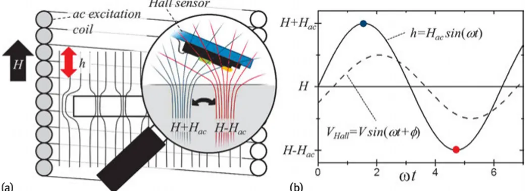
Fig. 2.6: (a) Schematic overview of the scanning susceptibility microscopy setup. A
superconduct-ing sample is placed in a dc magnetic field, H, generated by a superconductsuperconduct-ing coil surroundsuperconduct-ing a collinear copper coil generating an ac field hac(t). The time-averaged magnetic field profile due to the present vortices and the screening currents is schematically shown by the black lines. The mag-nifying glass provides a closer look at the induced ac vortex motion. When the drive is small, the ac magnetic field induces a periodic force on the vortices, shaking them back and forth. A Hall sensor picks up locally the associated time-dependent Hall voltage, VHall. (b) A lock-in amplifier, provided with both hac(t) as a reference and VHall, allows one to extract both the in-phase, B
z(x, y), and the out-of-phase, Bz(x, y), components of the local magnetic response.
in-phase component, μ1(x, y), to the local inductive response, while the out-of-phase component, μ1(x, y), is related to microscopic ac losses.
2.2.2 SSM on a superconducting strip, response of individual vortices
In the following section, we will, as a proof of concept, use SSM to analyze the ac re-sponse of the Pb ribbon discussed before. The interpretation of the measured local response functions μ1(x, y) and μ1(x, y) and the analysis of their dependencies upon varying thermodynamic variables (temperature, dc magnetic field) or the drive ampli-tude will be discussed. As the signal picked up by the Hall probe contains different contributions, arising from the screening currents, the vortex signals and the external field itself, the measured local linear ac response is also determined by all contribut-ing factors. This particular sample design allows us to map the spatial dependence of the linear response to hac(t), covering the whole width of the sample in a single scanning area, including the Meissner response at the sample border and the vortex motion deeper into the ribbon volume.
2.2.2.1 Temperature dependence of the macroscopic ac response
Before we discuss in detail the response in the whole scan area, let us first discuss the temperature variation of μ1(x, y) and μ1(x, y) picked up by the Hall cross located ∼ 1 μm above the center of a zero-field cooled (ZFC) 7 μm wide Pb ribbon, see Fig-ure 2.7. An ac amplitude of 0.1 mT and a frequency of f= 77.123 Hz are used for this measurement. This dependence is identical to the temperature dependence observed in macroscopic ac-susceptibility experiments. It is clear that the Pb ribbon exhibits a superconducting transition at Tc= 7.20 K. For temperatures below Tca diamagnetic response is observed, 0< μ1(x, y) < 1, meaning the ribbon screens out the applied field. Above Tc, μ1(x, y) ≈ 1, meaning the ac magnetic field penetrates completely as expected for this low frequency for a normal metal. μ1(x, y) is initially zero, goes through a maximum, and reduces to a zero value near Tc.
Figure 2.8a shows an SHPM image of a vortex distribution prepared by a field cool (FC) in H= 0.13 mT and at T = 6.7 K. After preparing the state, a SHPM image is ob-tained while an external field with hac = 0.1 mT and f = 77.123 Hz, is continuously applied. The scan speed is chosen properly, 1 μm/s, to ensure that the integration time at every pixel (125 ms) is much larger than the period of the applied ac field (13 ms). As one image has 128 by 128 pixels, the time for a single scan takes 73 minutes. The resulting vortex distribution obtained by performing a FC experiment, corresponds to a frozen vortex structure nucleated close to Tc[31]. The FC process forces vortices to nucleate at the strongest pinning sites and results in a nonsymmetrical vortex distri-bution. The external ac field shows up as an additional monochromatic noise in the SHPM images getting more pronounced for temperatures close to Tc. However, for all
Fig. 2.7: In-phase (χ’) and out-of-phase (χ”) ac signal picked up by the Hall cross located at the
cen-ter of a 7 μm stripe, using an ac amplitude of 0.1 mT and a frequency of f= 77.5 Hz.
investigated temperatures the average vortex positions do not change, indicating that for hac = 0.1 mT the resulting average vortex response is limited to displacements below the experimental spatial resolution.
2.2.2.2 Probing the ac response with single vortex resolution
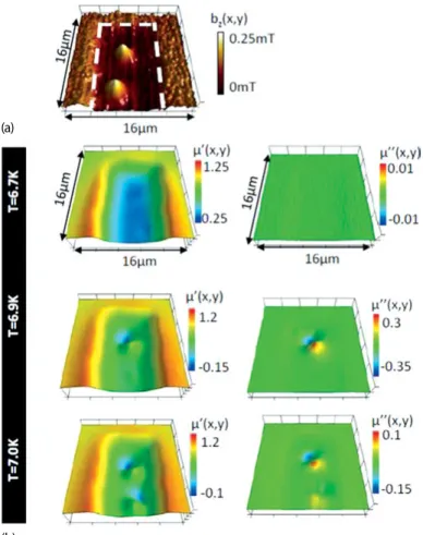
Figure 2.8b shows a representative set of simultaneously acquired SSM images of
μ1(x, y) (left column) and μ1(x, y) (right column), respectively describing the
induc-tive and dissipainduc-tive response, when the temperature is decreased progressively from
T= 6.7 K to T = 7 K.
Local inductive response. A first straightforward observation is that at the edges of the scan area, meaning relatively far away from the Pb ribbon, the local induction is equal to the applied ac magnetic field hac(t) as μ1(x, y) = 0 and μ1(x, y) = 1. A clear paramagnetic response, μ1(x, y) > 1, is visible at the edge of the Pb ribbon, where the response is dominated by the induced screening currents. This enhancement of the external ac field is caused by a strong demagnetizing effect resulting from the thin film sample geometry [32]. Upon entering the volume of the ribbon, we observe an increasing diamagnetic response as hac(t) gets shielded by the screening currents. At the center of the Pb ribbon, a maximum diamagnetic response due to the screening current of μ1(x, y) = 0.27 at T = 6.7 K is reached, indicating an incomplete field expulsion.
Fig. 2.8: (a) Scanning Hall probe microscopy image of the local induction, Bz(x, y), acquired dur-ing shakdur-ing with an external applied ac field of amplitude, hac = 0.1 mT, and with frequency,
f = 77.123 Hz at a temperature of T = 6.7 K. The initial vortex distribution is obtained by performing
a field cool in an external applied dc magnetic field, H= 0.13 mT. The white dashed line indicates the border of the Pb ribbon.(b) Simultaneously acquired maps of the real part of the relative per-meability, μ1(left column) and the imaginary part of the relative permeability, μ1(right column), for different temperatures:(top to bottom) T= 6.7 K, 6.9 K and 7.0 K.
Within the ribbon volume the induced screening currents, j(t), will periodically shake the vortices, with a force: fL(t) = j(t) × ϕ0. The ac dynamics of the vortices will
crucially depend on the thermodynamic parameters of the superconducting system and the properties of the drive. As shown in Figure 2.8b, the fingerprint of their mo-tion in the SSM images, consists of two distinct unidirecmo-tional spots of opposite polar-ity surrounding the equilibrium vortex position. The inductive response can be easily interpreted. An area exhibiting a signal exceeding the ac response of the screening currents, μ1(x, y) > μ1(x, y)s, corresponds to a vortex, carrying an intrinsic positive
local induction, moving in-phase with hac(t) within this area. A region exhibiting a signal lower than the ac response of the screening currents, μ1(x, y) < μ1(x, y)s, in
some cases resulting even in a local negative permeability, μ1(x, y) < 0, indicates that
bz(x, y, t) increases (decreases) upon decreasing (increasing) instantaneous hac(t), corresponding to a vortex moving in anti-phase with hac(t) within this area. A simi-lar unique local negative μ1(x, y) response, but on a substantially larger spatial scale, has been observed in the ac dynamics of flux droplets in the presence of a geometrical barrier [30].
From general considerations, neglecting the demagnetizing field, an overall in-tegrated response between zero and one is expected for⟨μ1⟩. Note however, that the meaning of the complex permeability as a macroscopic thermodynamic variable is lost in this local limit. Upon integrating the local signal over the whole scan area the ex-pected non-negative response for⟨μ1⟩ and ⟨μ1⟩ is recovered. This connection between ⟨μ1⟩ as the integrand of the ‘local’ permeability, μ1(x, y), which is directly related to the microscopic vortex dynamics, is used in theoretical models to explain the finger-prints of different dynamical vortex lattice regimes in measurements of the global ac-susceptibility and can be studied now directly by SSM. Furthermore, the particular depth and shape of the local pinning potential that each vortex experiences has a pro-found effect on the ac dynamics, i.e., at T= 6.9 K only one of the two vortices present in our scan area is shaking.
Local dissipative response. An important observation in Figure 2.8b is that the shielding currents do not show any contributing signal in μ1(x, y) for all tempera-tures, indicating that they are, within our experimental resolution, perfectly in-phase with the ac excitation and therefore they are nondissipative. In sharp contrast to the screening currents’ response, the vortices do leave a fingerprint in μ1(x, y) for suf-ficiently high temperatures. As such, the oscillating magnetic stray field produced by an harmonic motion of the vortices exhibits an of-phase component. The out-of-phase response disappears for T < 6.8 K, here the ac response of the vortices is weak and, within the experimental resolution, perfectly in-phase. An illustration of all forces working on a single vortex inside the Pb ribbon is shown in Figure 2.9. In this case the parabolic caging potential is the result of the interplay between the vor-tex and the screening currents, while the additional roughness is induced by sample inhomogeneity. The presence of these modulations at length scales much smaller than the distance traveled in this experiment (≈ 500 nm) has been observed in later exper-iments using different high-resolution scanning probe techniques [6, 7]. The solution of the resulting equation of motion is given by Equation (2.33) and directly shows that the out-of-phase component in the linear response can be induced by two different dissipative mechanisms: viscous damping or thermal fluctuations.
This viscous damping process has a typical short characteristic time of the order of τp= η/αL≤ 0.1 μs [25]. For the applied low driving frequency, f = 77.123 Hz, the restoring force dominates over the viscous drag force, as ω≪ 1/τpand this term can be neglected. The term i/ωτ1in Equation (2.33) is related to thermally activated vortex
Fig. 2.9: Schematic representation of the forces working on a single vortex in the Pb ribbon at time
t1as described by Equation (2.17). In this picture αLdetermines the potential well of a single vor-tex, no longer a statistical average, and is the result of the interplay between the vortex and the screening current.Uroughis an additional finer structure in the effective potential induced by sam-ple inhomogeneity. In case thermal excitations (FTh) are comparable toUrough, thermal relaxation following the classical idea of Anderson and Kim [35], becomes important.
hopping across an effective activation barrier, following the classic ideas of Anderson and Kim [35] and results from thermal excitations. This activated hopping process is typically associated with longer characteristic time scales [36]. Under certain condi-tions it is expected to contribute substantially in our low-frequency SSM experiment. It is interesting to make here a small parenthesis to discuss the linear response of this vortex system. If we neglect the viscous damping force at low driving frequency, we can rewrite Equation (2.33) in the following way,
x(t) = F0|χ(ω)| cos(ωt + θ(ω)) with χ(ω) = ( 1 αL− i ωτ1αL) (2.42) Here x(t) is the vortex position and the complex number χ(ω) describes the response of the vortex system. As in Section 2.1.1, we can parameterize the solution by the am-plitude and the phase of χ(ω) as:
|χ(ω)| = 1 αL√1 + 1 (ωτ1)2 and tan θ(ω) = 1 ωτ1 (2.43) In both expressions for the amplitude and the phase lag, the term ωτ1appears explic-itly. For a fixed characteristic time τ1the deviation from pure reversible motion arises when ωτ1approaches 1. It implies that the driving frequency approaches the charac-teristic time for thermally activated motion and the vortex motion will be dominated by this process. As a result, a phase lag appears between drive and vortex displace-ment. When the driving frequency is much larger, ωτ1 ≫ 1, but still small enough to neglect viscous damping, ωτp ≪ 1, the motion reduces to Campbell’s reversible
vortex motion. In this frequency regime thermally activated motion will contribute negligibly to the motion properties of a vortex. The situation where ωτ1 < 1 can not be described within a linear response, as in this case, the response is strongly non-linear [22] and the above equations do not apply. In the reversible Campbell regime a one-to-one correspondence exists between a vortex and a driven damped harmonic oscillator as discussed in Section 2.1.1, within the limits ω≪ ω0and ω≪ (k/η).
Before we continue with the interpretation of the measured temperature depen-dence of the vortex response, we show explicitly that the measured phase with SSM corresponds to the phase-lag in Equation (2.43). We denote by Bv
z(xi, yi, t) the
mag-netic induction carried by a single vortex, shaking back and forth around its equilib-rium position, ri0. We assume that the vortex is driven by a small ac excitation in a
way that ri= (xi, yi) oscillates about ri0. In this situation, we can expand Bvz(xi, yi, t)
in a Taylor series around ri0. Without loss of generality, we can choose the x-axis
par-allel to the applied drive. We further assume that the vortex displacement is parpar-allel to the force, which is valid for a linear response in isotropic media. In this case, vortex motion is restricted to the x-direction and the expansion can be performed in powers of δxi= xi− xi0: Bvz(x − xi(t)) = ∞ ∑ p=0 1 p! ∂pBvz ∂xpi |xi0δx p i (2.44) = Bv−dc z (x) − ∂Bv−dc z ∂x δxi+ 1 2 ∂2Bv−dc z ∂x2 δx 2 i + O (δx3i) (2.45)
With Bvz−dc(x) the magnetic field distribution of the vortex without being excited. No-tice that the change of sign of the odd terms of the expansion due to changing xiby
x in the derivatives. If we assume that the vortex displacement can be expressed as δxi= |χ(ω)| cos(ωt + θ(ω)), as in Equation (2.42), we obtain for the in-phase and
out-of-phase response, Bzv= 1 T∫ dt cos(ωt)Bz(x, y, t) = −|χ(ω)| ∂Bv−dc z ∂x cos(θ(ω)) (2.46) Bzv= 1 T∫ dt sin(ωt)Bz(x, y, t) = |χ(ω)| ∂Bvz−dc ∂x sin(θ(ω)) (2.47)
Note that in the case of a diluted vortex distribution, Bv−dc
z expands over distances
of the order of the penetration depth. This scale exceeds, in the linear regime, typical vortex displacements and hence one can safely keep the leading order terms. These re-sults lead to the conclusion that the measured modulus SSM signal, √(Bzv)2+ (Bzv)2, is directly related to the amplitude of vortex motion, with a proportionality constant given by the gradient of Bv−dc
z in the direction of the driving force. Furthermore, the
mo-tion and the Lorentz drive. |χ(ω)| = (∂Bvz−dc ∂x ) −1 √(B z v )2+ (Bz v )2 (2.48) tan(θ(ω)) = −B z v Bzv (2.49)
With these parameters the dependence on the probe position cancel out and should be homogeneous, apart from the places where ∂Bvz−dc/∂x = 0.
Let us use the above considerations to interpret the temperature dependence of the out-of-phase component of the vortex response. At low temperatures, when U(j) ≫
kBT and thermally activated flux motion can be neglected, τ1diverges exponentially and the ac response, x(t) = αLfL(t), is a pure reversible harmonic motion as described
by Campbell and Evetts [26]. This behavior explains the absence of a response in the SSM images of μr(x, y) for T < 6.8 K, while a response is still visible in μr(x, y). As the temperature rises, the thermal activation energy decreases and 1/ωτ1becomes ap-preciable, meaning thermally activated vortex jumps between metastable states come into play and contribute substantially to the vortex motion. This explains the observed out-of-phase component for T> 6.8 K. Figure 2.10 shows a zoom-in of the ac response of a single vortex for T = 6.9 K and the corresponding spatial dependence of the calculated phase, where we use a cutoff for| μr(x, y) |< 0.15 to limit the divergence of the arctangent function and we subtracted the contribution of the screening cur-rents in μr(x, y). As shown in Figure 2.10c, the obtained phase shift is θ = −0.5 rad. From Equation (2.43), the phase shift between the response and the drive is given by
θ= − arctan(1/τ1ω). As τp≤ 0.1 μs, we obtain a lower limit for the effective activation barrier height of U(j) ≥ 8.50 × 10⁻³eV∼ 14.3kBT, similar to typical average effective barrier heights found in the literature by macroscopic measurements [37].
Fig. 2.10: (a) Scanning susceptibility microscopy image of the real part of the relative permeability,
μrfor a single vortex upon shaking with an external ac magnetic field of amplitude, hac= 0.1 mT, and frequency f= 77.123 Hz at a temperature of T = 6.9 K. The initial vortex distribution is obtained by performing a field cool in an external applied dc magnetic field, H= 0.13 mT. (b) Simultaneously acquired map of the imaginary part of the relative permeability, μr. (c) Calculated spatial depen-dence of the negative phase angle.
The temperature dependence of the phase shift shows a maximum at T= 6.85 K. Optimal energy dissipation is expected when the driving frequency matches the char-acteristic frequency of our vortex system, i.e., when the resonant absorption condi-tion, ωτ1 = 1, is fulfilled. As the driving frequency is fixed, we approach or detune from the resonant absorption condition by changing τ1with temperature. The non-monotonic temperature dependence of the phase shift reflects the nontrivial temper-ature dependencies of the different factors contributing in τ1.
2.2.3 Examples of application of the SSM technique
In the previous sections we have shown concrete examples illustrating the power of the SSM technique for tracking the motion of individual vortices and to understand the dissipative mechanism involved during their displacement. Now we will present, in a rather concise way, further applications of the technique to a variety of interesting superconducting materials.
2.2.3.1 Imaging the dynamics of vortices and antivortices induced by magnetic microdisks
The microscopic static and dynamic behavior of vortex–antivortex pairs sponta-neously induced by Co/Pt micromagnets with out-of-plane magnetic moment in close proximity to a superconducting Pb film has been investigated via SSM by Kramer and co-workers in Reference [38]. Images of the obtained results are shown in Figure 2.11. Panel (a) corresponds to the static image obtained at zero field and with the disks fully magnetized (red spots). The presence of seven antivortices, three at the center and four at the rims of the scanning area can be distinguished as dark blue spots. This vortex configuration is then excited with a small ac field (hac= 0.02 mT) and the oscillation of each individual vortex is recorded by the SSM as shown in panel (b). It can be seen that two of the central antivortices strongly oscillate whereas no motion is detected for any vortex sitting on top of the magnetic disks. In panel (c) the two panels, (a) and (b), have been superimposed to better identify those vortices able to move. It is worth emphasizing that the SSM technique is able to detect only periodic motion between two points and therefore, the lack of signal associated with the rest of the antivortices can be either because they remain pinned or due to a nonperiodic trajectory during the ac excitation. By increasing the amplitude of the ac excitation (hac= 0.06 mT) eventually it is possible to shake the much more strongly pinned vor-tices on top of the disks. This is shown in panels (d) to (f), corresponding to a lower magnetic moment with only one antivortex present at the left side of the scanning area. In this case SSM has permitted us, for the first time, to unveil the difference in mobility between both vortex species.