HAL Id: hal-00397235
https://hal.archives-ouvertes.fr/hal-00397235v2
Submitted on 18 Feb 2014
HAL is a multi-disciplinary open access
archive for the deposit and dissemination of
sci-entific research documents, whether they are
pub-lished or not. The documents may come from
teaching and research institutions in France or
abroad, or from public or private research centers.
L’archive ouverte pluridisciplinaire HAL, est
destinée au dépôt et à la diffusion de documents
scientifiques de niveau recherche, publiés ou non,
émanant des établissements d’enseignement et de
recherche français ou étrangers, des laboratoires
publics ou privés.
Stochastic π-Calculus Framework
Loïc Paulevé, Morgan Magnin, Olivier Roux
To cite this version:
Loïc Paulevé, Morgan Magnin, Olivier Roux. Refining Dynamics of Gene Regulatory Networks in a
Stochastic π-Calculus Framework. Transactions on Computational Systems Biology, Springer, 2011,
XIII, pp.171-191. �10.1007/978-3-642-19748-2_8�. �hal-00397235v2�
Networks in a Stochastic π-Calculus Framework
Lo¨ıc Paulev´e, Morgan Magnin, Olivier Roux
IRCCyN, UMR CNRS 6597, ´
Ecole Centrale de Nantes, France
{loic.pauleve,morgan.magnin,olivier.roux}@irccyn.ec-nantes.fr
Abstract. In this paper, we introduce a framework allowing to model and analyse efficiently Gene Regulatory Networks (GRNs) in their tem-poral and stochastic aspects. The analysis of stable states and inference of Ren´e Thomas’ discrete parameters derives from this logical formalism. We offer a compositional approach which comes with a natural transla-tion to the Stochastic π-Calculus. The method we propose consists in successive refinements of generalised dynamics of GRNs. We illustrate the merits and scalability of our framework on the control of the differ-entiation in a GRN generalising metazoan segmentation processes, and on the analysis of stable states within a large GRN studied in the scope of breast cancer researches.
Changes since http://dx.doi.org/10.1007/978-3-642-19748-2_8 – Add a 6= b in V equation of Definition 9 (Hitless Graph).
1
Introduction
Modelling, analysis and numerical or stochastic simulations are a usual means to predict the behaviour of complex living systems such as interacting genes.
Regulations between genes (activation or inhibition) are generally represented by Gene Regulatory Network (GRN) graphs. However, a GRN graph is not enough to describe dynamics. In continuous frameworks such as ordinary dif-ferential equations, parameters for difdif-ferential equations are needed. In logical (or qualitative) frameworks such as boolean or discrete networks, dynamics are driven by Ren´e Thomas’ parameters or equivalent [1].
Hybrid modelling brings quantitative aspects — such as temporal or stochas-tic parameters — to logical modelling. In the field of formal languages, κ lan-guage [2] or Stochastic π-Calculus [3,4,5] bring theoretical Computer Science frameworks for biological modelling. In the field of formal verifications of bio-logical systems, frameworks like Time or Stochastic Petri Nets [6,7], Biocham [8], Timed Automata [9], Charon (Hybrid Modelling) [10] and Linear Hybrid Modelling [11] bring the first bricks for verifying and controlling dynamics of such systems.
Inference of temporal and stochastic parameters is still challenging as the domain of parameters is continuous and its volume generally grows exponen-tially with the number of genes. Compositional approaches, inherent to process algebras, aspire at reducing this complexity by allowing a local reasoning.
Our aim is temporal parameters synthesis for verifying formal properties on hybrid models.
Our contribution consists in the introduction of both temporal and stochastic parameters into process algebra models of GRNs through a new Stochastic π-Calculus framework: the Process Hitting framework.
Starting from a GRN without any other parameters, its largest dynamics are expressed in Process Hitting and then are refined to match the expected behaviour. Such a refinement is achieved by constructing cooperativity between genes and by creating stable states. As we will show, detecting stable states of a Process Hitting is straightforward, as well as infering the Ren´e Thomas’ discrete parameters K.
Moreover, the Stochastic π-Calculus naturally brings time and stochasticity into our Process Hitting framework. We introduce a stochasticity absorption
fac-tor to highlight either the temporal or stochastic aspect of reactions. The direct
translation of Process Hitting to the Stochastic π-Calculus allows simulations of such models by softwares like BioSpi [3] or SPiM [12].
Several points motivate the choice of the Stochastic π-Calculus framework for introducing the Process Hitting. The Stochastic π-Calculus can be consid-ered as a “low-level” process algebra: there are very few operators compared, for instance, to the Beta Workbench [13] or Bio-PEPA [14]. This makes the presentation of the Process Hitting as a Stochastic π-Calculus framework more generic. Moreover, the Stochastic π-Calculus comes with a bunch of established tools as previously cited and translations into various framework have already been formalized, such as to PRISM, a probabilistic model checking tool [15,16]. This paper is structured as follows. Section 2 introduces our framework and how it is used to build the generalised dynamics of a GRN. Section 3 presents dynamics refinement techniques and Section 4 shows how infering the Ren´e Thomas’ parameters leading to such dynamics. Introduction of both temporal and stochastic parameters within Process Hitting models is addressed in Sec-tion 5. The overall approach is illustrated by two applicaSec-tions in SecSec-tion 6. The first applies the refinement method to a toy GRN involved in biological segmen-tations phenomena. The temporal and stochastic parameters are then infered to bring a particular behaviour to the system. The second application shows the scalability of the Process Hitting framework by modelling a large GRN composed of 20 genes.
Notations Given a set S,
n
z }| {
S × · · · × S, will be abbreviated as Sn. If S is finite
and countable, we note |S| its cardinality. Given a n-tuple C, C[x/y] refers to the n-tuple C within the element y has been substituted by x. Belonging and cartesian product for n-tuples are defined similarly to sets. [xi; xi+n] refers to
2
Generalised Dynamics for Gene Regulatory Networks
First, we recall the basis of the Ren´e Thomas’ discrete modelling framework from which we designed our refinement approach. This method is described in subsections 2.2 and 2.3. This leads to a straightforward translation into the π-Calculus which makes it possible to express generalised dynamics of GRNs. 2.1 Gene Regulatory Networks
GRNs are often described by interaction graphs where nodes are genes with acti-vation and inhibition relations respectively represented by positive and negative edges [1,17].
In the discrete framework of Ren´e Thomas, each gene has at least two qual-itative levels. The influence of an activating (resp. inhibiting) gene on its target depends on a threshold value: when the level of the gene is greater or equal than the threshold, the gene holds a positive (resp. negative) effect; when the level of the gene is lower than the threshold, the gene holds a negative (resp. positive) effect [1].
Definition 1 (Gene Regulatory Network Graph). A Gene Regulatory Network graph is a triple (Γ, E+, E−) where Γ is the finite set of genes and
a−→ b ∈ Et + (resp. E−), t positive integer, if and only if the gene a above level t
is an activator (resp. inhibitor) for b. We note ai the level i of the gene a.
Given a GRN graph (Γ, E+, E−), the maximum qualitative level for gene
a ∈ Γ is noted ala where la is the highest threshold involved in its regulations:
la= max({t | ∃b ∈ Γ, a t
−
→ b ∈ E+∪ E−}) . (1)
We denote levels+(a, b) (resp. levels−(a, b)) the set of levels of a where a
effectively activates (resp. inhibits) b.
Definition 2 (Effective Levels). If a−→ b ∈ Et +, levels+(a, b) = [at; ala] and
levels−(a, b) = [a0; at−1]. If a t
−
→ b ∈ E−, levels+(a, b) = [a0; at−1] and
levels−(a, b) = [at; ala]. Else levels+(a, b) = levels−(a, b) = ∅.
2.2 The Process Hitting Framework
We want to describe the action of a gene at a given level on another one. If the gene a at a given level i is an activator for b, it has a positive action on b, meaning the level of b will tend to increase. Conversely if a at a level i′ is an inhibitor for b, it has a negative action on b and then the level of b will tend to decrease.
The action is “a at level i making b at level j increase (or decrease) to level k”. We say ai hits bj to make it bounce to bk and note this action ai→ bj bk.
In the process hitting framework, ai, bj, bk are refered as processes and a, b as
sorts. Sorts can represent genes, but also logical entities, as described in further
Definition 3 (Action). An action is noted ai→ bj bk where ai is a process
of sort a and bj 6= bk two processes of sort b. ai→ bj is the hit part, and bj bk
the bounce part. When ai= bj, such an action is refered as a self-action and ai
is called a self-hitting process.
In this paper, one and only one process of each sort is present at any instant. Hence, hits between different processes of a same sort are prohibited. The set of these living processes gives the state of the Process Hitting.
Definition 4 (Process Hitting). A Process Hitting PH is a triple (Σ, L, H): – Σ = {a, b, . . . } is the finite countable set of sorts,
– L =Qa∈ΣLais the set of states for PH, with La = {a0. . . ala} the finite and
countable set of processes of sort a ∈ Σ and la a positive integer, a 6= b ⇒
ai 6= bj ∀(ai, bj) ∈ La× Lb,
– H = {ai→ bj bk, · · · | (a, b) ∈ Σ2, (ai, bj, bk) ∈ La× Lb× Lb, bj6= bk, a =
b ⇒ ai= bj}, is the finite set of actions.
At a given state s ∈ L, an action ai→ bj bkis playable if both processes ai
and bj are present in s. When this action is played, the process bk replaces bj.
Definition 5 (Next States). Let (Σ, L, H) be a Process Hitting and s ∈ L be
one of its states. The set of the next possible states for s are computed as follows:
next(s) = {s[bk/bj] | ∃(ai, bj) ∈ s2, ∃bk∈ Lb, ai→ bj bk∈ H} .
Definition 6 (Stable state). Let PH = (Σ, L, H) be a Process Hitting and s ∈ L be a state, s is a stable state for PH if and only if next(s) = ∅.
2.3 Graphical Representations of a Process Hitting
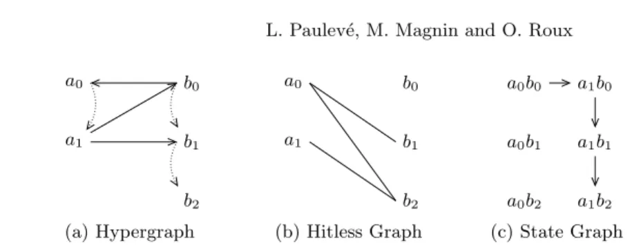
We set up two complementary graphical representations of a Process Hitting. The first one exhibits the actions between process levels, the second one points out the absence of hits between them. We finally define the State Graph of a Process Hitting. Figure 1 shows an instance for each of these three representa-tions.
Given a Process Hitting (Σ, L, H), its Hypergraph represents each action ai→ bj bk ∈ H by a directed hyperedge from ai to bk passing by bj. The hit
part (aito bj) is drawn as a plain edge and the bounce part (bjto bk) as a dotted
edge.
Definition 7 (Process Hitting Hypergraph). The Hypergraph of a Process
Hitting (Σ, L, H) is a couple (P, A) where P = Sa∈ΣLa are the vertices and
A ⊆ P3 the directed hyperedges given by A = {(a
i, bj, bk) | ai → bj bk∈ H}.
In the following we introduce a complementary representation we call Hitless
Graph. It will allow us to obtain extra results such as the stable states of a
relates two processes of different sorts if and only if they hit neither each other nor themselves. Vertices of a Hitless Graph may be split into n ≤ |Σ| partitions having no element inside related to each other: a partition is, for any sort, a subset of its processes without self-actions. Such a graph is called n-partite. Definition 8 (n-Partite Graph). A graph G = (V, E) is n-partite if and only
if V =Snk=1Vk, Vk6= ∅, ∀1 ≤ k, k′ ≤ n, Vk∩ Vk′ = ∅ and (ai, bj) ∈ E ⇒
∃1 ≤ k 6= k′ ≤ n, a
i∈ Vk∧ bj∈ Vk′.
Definition 9 (Hitless Graph). Given a Process Hitting PH = (Σ, L, H), its
Hitless Graph PH = (V, E) is defined as a non-directed graph where the vertices
V and edges E are computed as follows:
V = [
a∈Σ
{ai∈ La| ∀ai′ ∈ La ∄ ai→ ai ai′ ∈ H}
E = {(ai, bj) ∈ V2| a 6= b ∧∀bj′ ∈ Lb ∄ ai→ bj bj′ ∈ H
∧ ∀ai′ ∈ La ∄ bj → ai ai′ ∈ H} .
Property 1. By construction of V and E, PH is a n-partite graph, n ≤ |Σ|, where each partition is a subset of processes for one and only one sort and to each sort corresponds at most one partition.
We also define the n-cliques of a graph which are subsets of n vertices such that each element is related to each other.
Definition 10 (n-Clique). Given a graph G = (V, E), C ⊆ V is a |C|-clique
of G if and only if ∀(ai, bj) ∈ C2, {ai, bj} ∈ E.
Property 2. n-cliques of a n-partite graph have one and only one vertex in each
partition.
Finally, the State Graph of a Process Hitting represents the possible transi-tions between each couple of its states.
Definition 11 (State Graph). Given a Process Hitting (Σ, L, H), its State Graph is a directed graph S = (L, E ⊆ L2) with (s, s′) ∈ E ⇔ s′∈ next(s).
2.4 From Process Hitting to the π-Calculus
A main advantage of our approach is its natural translation to the π-Calculus. In this subsection we propose a method to translate any Process Hitting into a π-Calculus expression.
We briefly present the fragment of the π-Calculus which is sufficient for trans-lating a Process Hitting. The full syntax for π-Calculus and examples can be found in [5,18]. π-Calculus expressions compose two kinds of objects: indepen-dently defined processes and channels shared by some processes. A process P has the capability to output (resp. input) on a channel γ and then become P′,
a0 a1 b0 b1 b2 a0 a1 b0 b1 b2 a0b0 a1b0 a0b1 a1b1 a0b2 a1b2
(a) Hypergraph (b) Hitless Graph (c) State Graph
Fig. 1. Graphical representations for the Process Hitting PH = ({a, b}, {a0, a1} ×
{b0, b1, b2}, H) with H = {b0→ a0 a1, a1→ b0 b1, a1→ b1 b2}.
noted !γ.P′(resp. ?γ.P′). Output and input are synchronized operations, i.e. an
outputting process is blocked until another process inputs on the same chan-nel. A process can also execute an internal action (τ ), nil operation (0) or one amongst several (P′+ P′′).
Let PH = (Σ, L, H) be a Process Hitting. For each process ai of PH, a
π-Calculus process Aiis defined as follows. For each action ai→ bj bk ∈ H where
a 6= b, a new channel γαis created. The π-Calculus process Ai has the ability to
output on this channel and the π-Calculus process Bj has the ability to input
on this channel so as to become Bk (2). For each self-action ai→ ai aj ∈ H,
Ai has the ability to become Aj after performing an internal action τα(3).
Ai ::= X α=ai→ bj bk∈H a6=b !γα.Ai+ X α=bj→ ai ak∈H a6=b ?γα.Ak (2) + X α=ai→ ai ak∈H τα.Ak (3)
2.5 Generalised Dynamics for Gene Regulatory Networks
Our method to analyse GRNs takes benefit from the use of refinement techniques. Starting from the largest set of possible dynamics for the GRN, we gradually take into account only the specified behaviours and exclude the other ones, thus leading to a restrictive process.
We call this largest set of dynamics the generalised dynamics for the GRN graph. It is described by the following rules: the level of a gene increases (resp. decreases) if and only if at least one of its activators (resp. inhibitors) is present. The absence of activators is equivalent to the presence of one inhibitor.
Let G = (Γ, E+, E−) be a GRN graph. For all (a, b) ∈ Γ2, we build the set
of actions Hb
a from a to b reflecting the rules above:
– If a−→ b ∈ Et +, all processes of sort a below the threshold t hit all processes
of sort b but b0 to make them decrease to the level below. Moreover, all
make them increase to the level above: Hb
a = {ai→ bj bj−1| 0 ≤ i < t, 1 ≤ j ≤ lb}
∪ {ai′ → bj′ bj′+1| t ≤ i′ ≤ la, 0 ≤ j′ < lb} .
– If a−→ b ∈ Et −, the actions are defined similarly to the previous case except
for the bounce directions which are reversed:
Hba = {ai→ bj bj+1| 0 ≤ i < t, 0 ≤ j < lb}
∪ {ai′ → bj′ bj′−1 | t ≤ i′ ≤ la, 1 ≤ j′ ≤ lb} .
– If b = a and ∄c ∈ Γ, c−→ b ∈ Et −∪ E+, gene b lives in absence of activators:
all processes of sort b but b0 hit themselves to decrease to the level below.
Hbb = {bi→ bi bi−1| 1 ≤ i ≤ lb} .
– Obviously, if a−→ b /t ∈ E−∪ E+for any t and the previous case does not hold,
we define Hb a = ∅.
The Process Hitting for the generalised dynamics of G is given by
PH = (Γ, Y a∈Γ {a0, . . . , ala}, [ (a,b)∈Γ2 Hab) .
3
Refining Dynamics of Gene Regulatory Networks
We present two methods which aim at narrowing the set of dynamics of a Process Hitting for a GRN: the first one is based on cooperativity between genes, the other one deals with the knowledge of the stable states.
3.1 Cooperative Hits
Given two genes c and f regulating a gene a, the action of c on a may depend on the level of f : there exists a cooperativity between c and f on a. In discrete frameworks, the cooperativity is often described by a boolean function between genes levels [1,19]. We show how to build cooperativity within Process Hitting. Let (Σ, L, H) be a Process Hitting and σ ⊂ Σ be a set of sorts cooperating on a given process ak to make it bounce to ak′. The set of all states of the
cooperating sorts is denoted by S = Qz∈σLz. The subset of states where the
cooperativity is effective is defined by ⊤ ⊂ S.
For applying this cooperation, a new sort is added to the Process Hitting. This sort is called a cooperative sort and is refered as υ. The set of processes of sort υ is defined by Lυ= {υς, ∀ς ∈ S}. Each process ziof sort z ∈ σ hits processes
υς of the cooperative sort υ where zi ∈ ς to make it bounce to υ/ ς[zi/zj], zj ∈ ς.
We denote Hσ the set of such actions (4). In this way, the process of sort υ
The cooperativity between υ processes is added into the Process Hitting by replacing hits Hcoop from processes of sorts present in σ to ck (5) by hits H′coop
from processes of the cooperative sort υ selected in ⊤ (6). Hσ= {zi → υς υς[zi/zj] | ∀z ∈ σ, ∀(zi, zj) ∈ L
2
z, ∀υς∈ Lυ, zj∈ ς} (4)
Hcoop= {zi → ak ak′ ∈ H | ∀z ∈ σ} (5)
H′coop= {υς→ ak ak′ | ∀ς ∈ ⊤} . (6)
The resulting Process Hitting is (Σ ∪ {υ}, L × Lυ, (H \ Hcoop) ∪ Hσ∪ H′coop).
Example 1. Let ({f, c, a}, {f0, f1} × {c0, c1} × {a0, a1}, H) be a Process Hitting
where {f1→ a0 a1, c0→ a0 a1} ⊂ H. The creation of a cooperativity
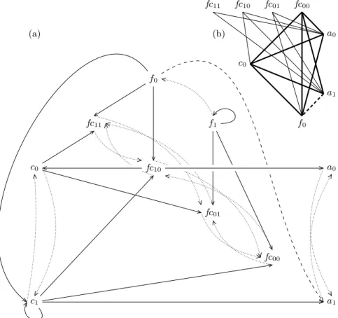
be-tween f1and c0 on a0 (σ = {f, c}, ⊤ = {f1c0}) is illustrated by Figure 2.
c0 c1 f1 f0 a0 a1 f1 f0 c0 c1 a0 a1 fc01 fc00 fc11 fc10
Fig. 2. Construction of a cooperative hit between f1 and c0 on a0 (thick lines):
σ= {f, c}, ⊤ = {f1c0}, υ = fc. fc01stands for the process corresponding to the state
f0c1 of the cooperating processes σ.
3.2 Stable State Pattern
Given a Process Hitting (Σ, L, H), we prove the |Σ|-cliques of its Hitless Graph are exactly its stable states. Thus, stable states may be created by removing from the Process Hitting the very hits that make such patterns appear.
Theorem 1. Let PH = (Σ, L, H) be a Process Hitting and PH its Hitless
Graph. A state s ∈ L is stable if and only if s is a |Σ|-clique for PH.
Proof. By definition, next(s) = ∅ if and only if there is no hit between any
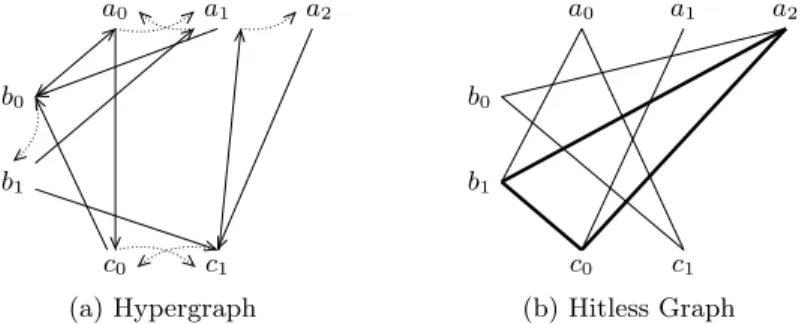
couple of processes present in s. This is equivalent to have s a clique of PH. Figure 3 shows an instance of Process Hitting having one stable state. We outline an algorithm for finding the n-cliques of a Hitless GraphPH = (V, E) where n = |Σ|.
Thanks to Prop. 1, we split V into n partitions corresponding to each process: V = ∪a∈ΣVa, Va ⊆ La. If one of this partition is empty, there can not be
n-cliques as it requires to have at least one vertex in each partition. We will assume Va6= ∅, ∀a ∈ Σ.
For each partition a ∈ Σ and each vertex ai ∈ Va, we define Eabi = {bj ∈
Vb | (ai, bj) ∈ E} for each other partition b ∈ Σ, b 6= a, the set of vertices in Vb
related to ai. If there exists b ∈ Σ such that Eabi = ∅, the vertex ai is removed
from candidates as it can not belong to a n-clique. Finally, we set Ea
ai= {ai}.
Once this pruning is performed, we enumerate potential n-cliques. To reduce this enumeration, we choose the partition a sharing the least number of edges. For each vertex ai∈ Va we test for all s ∈Qb∈ΣEbai if s is a clique ofPH.
For instance in Figure 3(b), a1 is removed from the Hitless Graph (Eab1 = ∅),
the partition associated to c is chosen (involved into only 4 edges), two states are tested: a0b0c1and a2b1c0 and the latter reveals to be the only 3-clique.
a0 a1 a2 b0 b1 c0 c1 a0 a1 a2 b0 b1 c0 c1
(a) Hypergraph (b) Hitless Graph
Fig. 3.A Process Hitting represented by its Hypergraph (a) and its Hitless Graph (b). The Hitless Graph contains only one 3-clique between a2, b1 and c0 (thick lines): this
is the only stable state of this system.
4
From Process Hitting to Ren´
e Thomas’ Parameters
A Ren´e Thomas’ discrete parameter gives the attractor levels for a gene when its regulators are in a given configuration. Many frameworks and tools dedicated to the study of GRNs take the full set of Ren´e Thomas’ parameters as essential input [1,9,11]. In this section, we give a formal method to infer Ren´e Thomas’ parameters for a GRN modelled in the Process Hitting framework.
Let (Γ, E+, E−) be a GRN graph. A Ren´e Thomas’ parameter Ka,A,B, a ∈
Γ, A ∪ B ⊆ Γ, A ∩ B = ∅, gives the interval of attracting levels for a when genes in A are activating a and genes in B are inhibiting a. In this configuration, if the level of a is in Ka,A,B, then it will never change; otherwise the level of a will
tend to a level in Ka,A,B.
Let (Σ, L, H) be a Process Hitting where sorts are standing either for genes or for cooperative sorts, i.e. Σ = Γ ∪ {σ1, . . . , σu} with ∀1 ≤ v ≤ u, σv ⊂ Γ .
Let Ka,A,B be the Ren´e Thomas’ parameter to infer. For each sorts b ∈ A ∪ B,
its context Cb
a,A,Bis defined as the subset of processes Lb imposed by the Ren´e
Thomas’ parameter: if b ∈ A (resp. B) only processes corresponding to positive (resp. negative) effective levels (Def. 2) are allowed. For each process b ∈ Γ
not regulating a (i.e. b /∈ A ∪ B), its context Cb
a,A,B is simply Lb (7). The
context Cσ
a,A,B for cooperative sorts σ ∈ {σ1, . . . , σu} is the set of states of its
representatives in their context (8).
∀b ∈ Γ, Ca,A,Bb = levels+(b, a) if b ∈ A, levels−(b, a) if b ∈ B, Lb otherwise. (7) ∀σ ∈ {σ1, . . . , σu}, Cσ a,A,B= {σς| ∀ς ∈ Y b∈σ Cb a,A,B} . (8)
We denote Ha,A,B the subset of the set of actions H on a that may be
performed by processes of the context of any sort (9). A process of sort a is reachable if it belongs to the context of a or is the result of any action in Ha,A,B.
The set of such processes is noted L?
a,A,B (10). The set of reachable processes
of sort a not hit by any other processes is noted L∗
a,A,B (11). Thus, as long
as present processes are in the context of their sort, if a process of sort a is in L∗
a,A,B, it will not be bounced. In this way, L∗a,A,B is called the set of focal
processes of a.
Ha,A,B= {bi→ aj ak ∈ H | bi ∈ Ca,A,Bb ∧ aj∈ Ca,A,Ba } (9)
L?
a,A,B= Ca,A,Ba ∪ {ak| ∀bi→ aj ak ∈ Ha,A,B} (10)
L∗a,A,B= L?a,A,B\ {aj| ∀bi→ aj ak ∈ Ha,A,B} . (11)
Finally, we check that the focal processes are attractors, i.e. all actions Ha,A,B
make processes of sort a bounce in the direction of the focal processes. If such a condition is satisfied, the focal processes correspond to the value of the requested Ren´e Thomas’ parameter. We point up that all these operations are linear with the number of actions in the Process Hitting.
Condition 1 (Focal processes are attractors). ∀bi → aj ak∈ Ha,A,B, ∀af ∈
L∗
a,A,B, |f − k| < |f − j| .
Property 3. If L∗
a,A,B satisfies Cond. 1, L∗a,A,Bis an interval.
Proof. If L∗
a,A,B = {af, . . . , af′} is not an interval, there exists bi→ aj ak ∈
Ha,A,B such that f < j < f′. If Cond. 1 applies, we have |f − k| < |f − j| ⇒
k < j ⇒ |f′− k| > |f′− j| which contradicts Cond. 1.
Theorem 2. If L∗
a,A,B6= ∅ and Cond. 1 holds, then Ka,A,B= L∗a,A,B .
Proof. By construction of L∗
a,A,B and application of Cond. 1 and Prop. 3, it
immediately appears that if L∗
a,A,B6= ∅, it is the set of attracting levels for a.
Consequently, there might exist configurations without any correspondence with Ren´e Thomas’ parameters. First, L∗
a,A,B= ∅ means the gene a is unstable
in the fixed context, i.e. its level is changing forever. Second, Cond. 1 is violated when there exists opposite focal processes, i.e. the fate of a is not deterministic.
One of the main reasons for non-determinism of Process Hitting is the absence of cooperativity between hits to a same target which may then independently be bounced to both higher and lower processes. We leave as an open question the problem to know whether such unstable and/or non-deterministic dynamics are biologically relevant.
5
Temporal and Stochastic Parameters
Further dynamics refinements may be achieved by taking into account the tem-poral and stochastic dimensions of biological reactions. On the one hand, we may consider the probability of a reaction to occur at a given state. By introducing stochastic parameters into discrete models, we aim at computing the probabil-ity of observing an expected behaviour. On the other hand, because they are faster, some reactions always apply before others. By introducing temporal pa-rameters into discrete models, we aim at reducing their dynamics to match such behaviours.
5.1 From Process Hitting to the Stochastic π-Calculus
The Stochastic π-Calculus [20] adds the capability to attach use rates to channels and internal actions of the π-Calculus. This gives a natural introduction for temporal and stochastic aspects in our Process Hitting framework.
A use rate controls both the duration and the probability of a reaction (com-munication on a channel or internal action). It is associated to a probability distribution for firing reaction along the time. The usual probability distribu-tion is the exponential one, allowing efficient simuladistribu-tions through a Gillespie-like algorithm [12,21]. This is the one we consider for the rest of this paper.
The probability along time t of firing a reaction with use rate r is given by F (t) = 1 − e−rt. The average duration of this reaction is r−1 with a variance of r−2. When x reactions are possible having use rates of r1, . . . , rx respectively,
the probability that the yth reaction is fired is given by ry
r1+···+rx.
The translation of Process Hitting (Σ, L, H) into the Stochastic π-Calculus is the same as the one presented in Section 2.4. Additionally, to each channel γα, or internal action τα, a use rate rαis attached.
5.2 Stochasticity Absorption
Use rates are both temporal and stochastic parameters. Nonetheless, these two aspects are closely tied: the lower a use rate is, the higher the variance around its mean duration is. We introduce a stochasticity absorption factor to control this variance to favour either the stochastic or the temporal behaviour of an action. We propose to replace the exponential distribution of a reaction with a rate r by the distribution of the sum of sa random variables each having an ex-ponential distribution of parameter r.sa. The resulting probability distribution is also known as the Erlang distribution. The average duration is unchanged:
(r.sa)−1sa = r−1, but the variance is divided by sa: (r.sa)−2sa = r−2sa−1. sa
stands for the stochasticity absorption factor. Based on the previously presented translation from the Process Hitting to the Stochastic π-Calculus, we supply a simple method to achieve this stochasticity absorption factor which do not re-quire to adapt simulation algorithms based on the memoryless property of the exponential law [22].
Basically, to each channel γα, or internal action τα, a use rate rα and a
stochasticity absorption factor saαis attached. To each component α of the sum
defined by the π-Calculus process Ai in the expressions (2),(3), a counter cα is
attached, initially, cα= 1. This counter is given as a parameter for Ai. As long
as this counter is not equal to saα, Aiis restarted and the counter is incremented
by one. When the counter reaches the stochasticity absorption factor value, the next process replaces Ai, having all its counters reset to 1. Let (Σ, L, H) be a
Process Hitting, for each process ai of PH, a π-Calculus process Ai is defined
as follows. Ai(˜c) ::= X α=ai → bj bk∈H a6=b !γα.Ai(˜c) + X α=bj→ ai ak∈H a6=b [cα< saα]?γα.Ai(˜c[cα+ 1]) + [cα= saα]?γα.Ak(˜1) + X α=ai→ ai ak∈H [cα< saα]τα.Ai(˜c[cα+ 1]) + [cα= saα]τα.Ak(˜1) where ˆc = c1, . . . , cn with n = |{bj → ai ak ∈ H}|. ˆc[cα+ 1] = c1, . . . , cα+
1, . . . , cn. Ak(˜1) is an abbreviation for the recursive call to Akwith all parameters
set to 1. [cond]π.P stands for an action π enabled only when cond is satisfied.
6
Applications
6.1 Metazoan Segmentation
In this section, we illustrate our method and its benefits on a case study in which our aim is to control the final state of the corresponding GRN. The GRN we chose has been established in silico by Fran¸cois et al. [23] but in a differ-ential equations framework. It aims at generalizing a common motif present in biological segmentation networks such as the Drosophila.
The GRN (Figure 4(a)) is composed of three genes. A wavefront gene f activates the gap-gene a whose products are responsible or stripes. Gene f also activates a gene c whose products repress the gene a. The auto-inhibition of c generalizes a chain of repressors on a. The apparition of stripes has to be regular. We attach to each gene two processes representing their qualitative levels (missing or present) — for instance c0(absence) and c1 (presence) are processes
for c. When f switches off, c goes to process c0and a has two fates, ending either
at process a0 or a1. We are interested in controlling the final process for a.
The Process Hitting for generalised dynamics of the GRN (Section 2) is computed first. Figure 4(b) shows its hypergraph. The specification of dynamics implies two cooperative hits in the Process Hitting: first, c0 needs products
of f to bounce to process c1; second, expression of a only increases if both
f activates it (i.e. process f1 is present) and c does not inhibit it (i.e. c0 is
present). Consequently, we create a cooperative sort fc reflecting the state of f and c (Section 3.1) and replace the independent hits from c0and f1to c0and a0
by hits from fc10. The resulting Process Hitting is represented in Figure 5(a).
By looking at the Hitless Graph of the Process Hitting (Figure 5(b)), only one stable state is present: f0c0fc00a0. The stability of the state f0c0fc00a1 is
controlled by the absence of inhibition by f0 on a1. By removing the action
f0→ a1 a0from the Process Hitting, we make the state f0c0fc00a1stable. The
full set of corresponding Ren´e Thomas’ parameters for the genes a and c is inferred by applying the method depicted in Section 4. We get:
Ka,∅,{a,c,f }= 0 Ka,{a,c},{f } = 1 Kc,∅,{c,f }= 0
Ka,{a},{c,f }= 0 Ka,{a,f },{c} = 0 Kc,{c},{f }= 0
Ka,{c},{a,f }= 0 Ka,{c,f },{a} = 1 Kc,{f },{c}= 0
Ka,{f },{a,c}= 0 Ka,{a,c,f },∅= 1 Kc,{c,f },∅= 1 .
We are interested in controlling the final process of sort a — either a0 or
a1 — when f goes down to f0. Looking at the Process Hitting hypergraph on
Figure 5(a) and considering f0is present, we deduce that the more c1is present,
the more a1may be hit by c1to bounce to a0; similarly, the more fc10is present,
the more a0may be hit by it to bounce to a1. We tune actions only triggered by
f0: we reduce the presence of c1by increasing the rate of the action f0→ c1 c0
and extend the presence of fc10 by reducing the rate of f0→ fc10 fc00. This
leads to an increase of the probability for a to bounce to process a1.
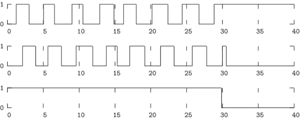
Finally, to obtain regular stripes, we set a high stochasticity absorption factor to actions responsible of the bounces of processes of sort c and a when f1 is
present. Figure 6 plots the evolution of the genes a,c and f during a simulation under SPiM [24] of the Process Hitting illustrated by Figure 5(a) with initial state f1c0fc10a0and a fast rate for the action f0→ c1 c0 compared to the rate
of c1→ a1 a0. The rate values have been arbitrarily choosen and respect the
infered relations between them. Appendix B.1 details the Process Hitting used for the simulation.
From the obtained simulation trace, we observe that f0hits c1 before c1had
time to hit a1: the final state is then f0c0fc00a1.
Thanks to the Process Hitting framework, it has been easy to build a qual-itative model of the biological system by refining the generalised dynamics of the GRN. Using a simple reasoning on the Process Hitting structure, relation between regulation delays to favour a final state have been infered. These results are coherent with those obtained using differential equations as done in [23].
f c a c1 c0 a1 a0 f0 f1 (a) (b)
Fig. 4.The starting Gene Regulatory Network graph (a), arrow-ended edges represent the positive regulations, and bar-ended edges the negative ones. All regulation thresh-olds are 1. The Process Hitting (b) for its generalized dynamics. Cooperativity between f1 and c0on a0 and c0will be applied in the same way as in example. 1.
c1 c0 f0 f1 a1 a0 fc11 fc10 fc01 fc00 c0 f0 a1 a0 fc11 fc10 fc01 fc00 (b) (a)
Fig. 5.The final Process Hitting (a) resulting from the refinement of the generalized dynamics depicted on Fig. 4(b). Cooperativity between f1 and c0 on a0 and c0 has
been built in the same way as in example 1. Absence of hit from f0to a1(dashed lines)
controls the presence of the relation between f0and a1in the Hitless Graph (b). If such
0 1 0 5 10 15 20 25 30 35 40 0 1 0 5 10 15 20 25 30 35 40 0 1 0 5 10 15 20 25 30 35 40
Fig. 6.Simulation of the Process Hitting for segmentation: evolution of the expressions of the gap-gene a (top), the autonomous clock c (middle) and the wavefront f .
6.2 ERBB Receptor-Regulated G1/S Transition
The aim of this section is to demonstrate the scalability of the refining approach on Process Hittings modelling large GRNs.
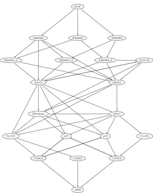
The selected GRN relates regulations between 20 genes. This GRN models the ERBB receptor-regulated G1/S transition involved in the breast cancer. It has been extracted from published data by Sahin et al. [25] and is reproduced in Figure 7. This network acts as an activation cascade for the gene pRB which controls the G1/S transition involved in cell divisions. The gene EGF then acts as an input of this cascade: when expressed, pRB will be potentially activated. Based on the literature, Sahin et al. have also established a set of logical rules controlling the activation of the various genes present in the network.
Starting from the GRN, its generalised dynamics expressed in Process Hitting is first computed. Then, cooperations between the different sorts are built from the logical rules. The Process Hitting obtained contains 670 actions and stands for 264 (≈ 2.1019) states that has hopefully not be built. This model is fully
detailled in Appendix B.2.
The computation of all the stable states present in the dynamics is done using the algorithm sketched by Section 3.2. It results in 5 stables states (also detailled in the appendix) that are computed in less than one second.
It is worth noticing that no assumption is made on the initial state of the system. All the stable states of the model are computed. This is a major differ-ence with the approach presented in [25] where only dynamics starting from a fixed state can be studied.
7
Conclusion
We introduced the Process Hitting framework for modelling qualitative dynamics of GRNs with temporal and stochastic features. Temporal and stochastic
param-EGF
ERBB2
ERBB1 ERBB3
ERBB1 2 ERBB1 3 ERBB2 3 IGF1R
MEK1 AKT1 ERalpha MYC CycD1 p27 p21 CycE1 CDK6 CDK2 CDK4 pRB
eters determine probabilities, durations and temporal variance of reactions in the model. We exhibited a direct translation from Process Hitting to the Stochastic π-Calculus. Detection of stable states and inference of Ren´e Thomas’ parame-ters for dynamics derive from this framework. The methods we offered work by successive refinements of generalised dynamics for GRNs, by specifying both the cooperativity between genes and the expected stable states. We illustrated this method by inferring temporal parameters for the dynamics of a GRN generaliz-ing metazoan segmentation processes (with the aim of controllgeneraliz-ing its final state). The scalability of the presented approach has been experimented on a Process Hitting modelling a GRN composed of 20 genes and computing its stable states. The Process Hitting brings a formal framework for progressively adding knowledge of the dynamics of a GRN by refining an abstracted behaviour. The compositionality of the framework and the presence of particular structure patterns lead to scalable methods for dynamics analyses (stable states, Ren´e Thomas’ parameters, etc.). Mainly, thanks to these Process Hitting patterns, it becomes possible to perform a local analysis, which has the major advantage to prevent us from exploring the full state and parameter space.
In future works, we aim at identifying more Process Hitting patterns leading to the emergence of particular behaviours (e.g. oscillations) and especially hybrid patterns coupling both discrete structure and continuous temporal and stochas-tic parameters. The verification of Process Hittings could be performed by using a translation into Petri Nets or into PRISM. Translating Process Hittings into more sophisticated process aglebras (Beta Workbench, Bio-PEPA, etc.) may also be of interest. Finally, techniques have to be developed to infer automatically temporal and stochastic parameters of Process Hittings modelling GRNs. Supplementary Material
The Process Hitting compiler to SPiM, a stable states computer and presented models are available at the following URL:
http://www.irccyn.ec-nantes.fr/~pauleve/processhitting-refining.tar. gz .
References
1. Richard, A., Comet, J.P., Bernot, G.: Formal Methods for Modeling Biological Regulatory Networks. In: Modern Formal Methods and Applications. (2006) 83– 122
2. Danos, V., Feret, J., Fontana, W., Harmer, R., Krivine, J.: Rule-Based Modelling of Cellular Signalling. In: CONCUR 2007 Concurrency Theory. (2007) 17–41 3. Priami, C., Regev, A., Shapiro, E., Silverman, W.: Application of a stochastic
name-passing calculus to representation and simulation of molecular processes. Inf. Process. Lett. 80(1) (2001) 25–31
4. Kuttler, C., Niehren, J.: Gene regulation in the pi calculus: Simulating cooper-ativity at the lambda switch. Transactions on Computational Systems Biology 4230(VII) (2006) 24–55
5. Blossey, R., Cardelli, L., Phillips, A.: A compositional approach to the stochastic dynamics of gene networks. Transactions in Computational Systems Biology 3939 (Jan 2006) 99–122
6. Popova-Zeugmann, L., Heiner, M., Koch, I.: Time petri nets for modelling and analysis of biochemical networks. Fundamenta Informaticae 67(1) (2005) 149–162 7. Heiner, M., Gilbert, D., Donaldson, R.: Petri Nets for Systems and Synthetic Biology. In: Formal Methods for Computational Systems Biology. (2008) 215–264 8. Rizk, A., Batt, G., Fages, F., Soliman, S.: On a continuous degree of satisfaction of temporal logic formulae with applications to systems biology. In Heiner, M., Uhrmacher, A., eds.: Computational Methods in Systems Biology. Volume 5307 of Lecture Notes in Computer Science. Springer Berlin / Heidelberg (2008) 251–268 9. Siebert, H., Bockmayr, A.: Incorporating time delays into the logical analysis of gene regulatory networks. In Priami, C., ed.: Computational Methods in Systems Biology. Volume 4210 of Lecture Notes in Computer Science. Springer Berlin / Heidelberg (2006) 169–183
10. Alur, R., Belta, C., Kumar, V., Mintz, M., Pappas, G.J., Rubin, H., Schug, J.: Modeling and analyzing biomolecular networks. Computing in Science and Engi-neering 4(1) (2002) 20–31
11. Ahmad, J., Bernot, G., Comet, J.P., Lime, D., Roux, O.: Hybrid modelling and dynamical analysis of gene regulatory networks with delays. Complexus 3(4) (2006) 231–251
12. Phillips, A., Cardelli, L.: Efficient, correct simulation of biological processes in the stochastic pi-calculus. In: Computational Methods in Systems Biology. Volume 4695 of LNCS., Springer (2007)
13. Dematte, L., Priami, C., Romanel, A.: The Beta Workbench: a computational tool to study the dynamics of biological systems. Brief Bioinform (2008) bbn023 14. Ciocchetta, F., Hillston, J.: Bio-pepa: A framework for the modelling and analysis
of biological systems. Theoretical Computer Science 410(33-34) (2009) 3065 – 3084
15. Hinton, A., Kwiatkowska, M., Norman, G., Parker, D.: PRISM: A tool for auto-matic verification of probabilistic systems. In: 12th International Conference on Tools and Algorithms for the Construction and Analysis of Systems. Volume 3920 of LNCS., Springer (2006)
16. Norman, G., Palamidessi, C., Parker, D., Wu, P.: Model checking probabilistic and stochastic extensions of the π-calculus. IEEE Trans. on Software Engineering 35(2) (2009) 209–223
17. Bernot, G., Cassez, F., Comet, J.P., Delaplace, F., M¨uller, C., Roux, O.: Seman-tics of biological regulatory networks. Electronic Notes in Theoretical Computer Science 180(3) (2007) 3 – 14
18. Milner, R.: A calculus of mobile processes, parts. I and II. Information and Computation 100 (1992) 1–77
19. Bernot, G., Comet, J.P., Khalis, Z.: Gene regulatory networks with multiplexes. In: European Simulation and Modelling Conference Proceedings. (Oct 2008) 423–432 20. Priami, C.: Stochastic π-Calculus. The Computer Journal 38(7) (1995) 578–589 21. Gillespie, D.T.: Exact stochastic simulation of coupled chemical reactions. The
Journal of Physical Chemistry 81(25) (1977) 2340–2361
22. Priami, C.: Stochastic π-calculus with general distributions. In: Proc. of the 4th Workshop on Process Algebras and Performance Modelling, CLUT. (1996) 41–57 23. Fran¸cois, P., Hakim, V., Siggia, E.D.: Deriving structure from evolution: metazoan
24. Phillips, A.: SPiM - Stochastic Pi Machine. (SPiM) http://research.microsoft. com/en-us/projects/spim.
25. Sahin, O., Frohlich, H., Lobke, C., Korf, U., Burmester, S., Majety, M., Mattern, J., Schupp, I., Chaouiya, C., Thieffry, D., Poustka, A., Wiemann, S., Beissbarth, T., Arlt, D.: Modeling ERBB receptor-regulated G1/S transition to find novel targets for de novo trastuzumab resistance. BMC Systems Biology 3(1) (2009)
A
Process Hitting Related Tools
This appendix briefly presents currently available implementations of tools ma-nipulating Process Hittings. They are available at the following URL:
http://www.irccyn.ec-nantes.fr/~pauleve/processhitting-refining.tar. gz .
Implemented in the OCAML language, these tools have a command-line user interline.
A.1 Process Hitting Specification
A basic language has been setup to specify Process Hitting using a text file. Main features are presented here, more details can be found in the provided archive. Full examples of Process Hitting specifications are given in Appendix B.
Sort definition A sort is declared by giving the process with the highest rank
(i.e. ala for the sort a, with the notations used in Section 2).
process a X
Action specification An action ai→ bj bkis added by the following instruction: a i -> b j k @ rate ~ absorption
Generalised dynamics of GRNs The GRN macro computes the generalised
dy-namics of the specified GRN according to Section 2.5. An activating (resp. in-hibiting) edge a−→ b from gene a to gene b active with a threshold X is notedX asa X -> + b(resp.a X -> - b).
Hereafter is an instance of the use of theGRN macro for the GRN having
activating edges a−→ b and a1 −→ a, and inhibiting edge b2 −→ b.1
GRN([a 1 -> + b; b 1 -> - a; a 2 -> + a ])
Refinement: cooperations The COOPERATIVITY([a1;...;an] -> b j k, [s1;...;sp])
macro creates a cooperative sort σ = {a1, . . . , an} for the bounce b
j bk. This
cooperation is effective for every state s1, . . . , sp.
The following instruction creates a cooperativity between sorts a and b to bounce process c0to c1 only if a1b0 or a0b1 are present.
Refinement: action removing An action ai→ bj bkcan be deleted by using the
macroRM:
RM({a i -> b j k})
A.2 Compiler to SPiM
This tool translates a Process Hitting specification into a SPiM model according to Section 5.2.
phc -spim <model.ph> <output.spi> A.3 Stable States Listing
The stable states of a Process Hitting are determined used an implementation of the algorithm sketched in Section 3.2. This algorithm computes the n-cliques of the hitless graph for the given Process Hitting, where n is the number of sorts. The efficiency of this computation heavily relies on the order of sorts when building cliques. Currently, basic heuristics are used to select the order of the sorts. More sophisticated analyses may conduct to dramatically improve the efficiency of this algorithm.
This tool is compiled into the executable ph-stable-states and takes as argument the filename of the Process Hitting specification :
ph-stable-states <model.ph>
B
Process Hitting Examples
This appendix details the Process Hittings used in Section 6. They are specified in the language presented in the previous appendix.
B.1 Metazoan Segmentation
The following Process Hitting models the metazoan segmentation presented in Section. 6.1. Actions are specified separately and rates have been assigned to values matching the relations infered in the application case study. The
directive sampleand initial stateinstructions are of use for SPiM only. A result of
the execution of this Process Hitting translated into SPiM is given by Figure 6.
d i r e c t i v e sample 40.
process a 1 process c 1 process f 1 process fc 3 (* c o o p e r a t i v e sort {f , c } *) c 1 -> fc 0 1 @5 . c 1 -> fc 2 3 @5 . c 0 -> fc 1 0 @10 . c 0 -> fc 3 2 @5 . f 1 -> fc 0 2 @10 . f 1 -> fc 1 3 @10 . f 0 -> fc 2 0 @0 .1 f 0 -> fc 3 1 @0 .1
(* a c t i o n s on c *) fc 2 -> c 0 1 @0 .5~50 (* only if ( f1 , c0 ) *) c 1 -> c 1 0 @0 .5~50 (* a c t i o n s on a *) fc 2 -> a 0 1 @1 .~50 (* only if ( f1 , c0 ) *) c 1 -> a 1 0 @1 .~50 (* a c t i o n s on f *) f 1 -> f 1 0 @0 . 0 3 4 ~ 1 0 0 (* auto - off *) f 0 -> c 1 0 @0 .1 i n i t i a l s t a t e f 1 , c 0 , a 0
B.2 ERBB Receptor-Regulated G1/S Transition
The following Process Hitting results from the case study presented in Sec-tion 6.2. It starts by specifying the GRN depicted by Figure 7 to compute its generalised dynamics. The logical rules setup by Sahin et al. [25] are then applied by using sorts cooperativity.
This Process Hitting contains 670 actions and 264 (≈ 2.1019) states. Only
5 stable states exist and are determined in less than a second using the tool presented in the previous appendix.
Below is the list of stable states present in the Process Hitting. For each stable state, only genes at level 1 are written.
– AKT1, CDK2, CDK4, CDK6, CycD1, CycE1, EGF, ERBB1, ERBB1 2, ERBB1 3, ERBB2, ERBB2 3, ERBB3, ERalpha, MEK1, MYC, pRB.
– AKT1, CDK2, CDK4, CDK6, CycD1, CycE1, ERalpha, IGF1R, MEK1, MYC, pRB.
– AKT1, CDK2, CycE1, EGF, ERBB1, ERBB1 2, ERBB1 3, ERBB2, ERBB2 3, ERBB3, ERal-pha, MEK1, MYC.
– AKT1, CDK2, CycE1, ERalpha, IGF1R, MEK1, MYC.
– ∅ (all genes have level 0).
process AKT1 1
process CDK2 1 process CDK4 1 process CDK6 1 process CycD1 1 process CycE1 1
process EGF 1 process E R a l p h a 1
process ERBB1 1 process E R B B 1 _ 2 1 process E R B B 1 _ 3 1 process ERBB2 1 process E R B B 2 _ 3 1 process ERBB3 1 process IGF1R 1 process MEK1 1 process MYC 1 process p21 1 process p27 1
process pRB 1 GRN([
E R B B 2 _ 3 1 -> + AKT1 ; E R B B 2 _ 3 1 -> + MEK1 ; E R B B 2 _ 3 1 -> - IGF1R ; ERBB2 1 -> + E R B B 2 _ 3 ; ERBB2 1 -> + E R B B 1 _ 2 ; ERBB3 1 -> + E R B B 2 _ 3 ; ERBB3 1 -> + E R B B 1 _ 3 ;
CycE1 1 -> + CDK2 ;
MEK1 1 -> + CycD1 ; MEK1 1 -> + E R a l p h a ; MEK1 1 -> + MYC ; CDK4 1 -> + pRB ; CDK4 1 -> - p21 ; CDK4 1 -> - p27 ;
E R a l p h a 1 -> + CycD1 ; E R a l p h a 1 -> + IGF1R ; E R a l p h a 1 -> + p21 ; E R a l p h a 1 -> + MYC ; E R a l p h a 1 -> + p27 ;
MYC 1 -> + CycE1 ; MYC 1 -> - p21 ; MYC 1 -> + CycD1 ; MYC 1 -> - p27 ; CDK6 1 -> + pRB ;
ERBB1 1 -> + E R B B 1 _ 2 ; ERBB1 1 -> + E R B B 1 _ 3 ; ERBB1 1 -> + AKT1 ; ERBB1 1 -> + MEK1 ;
E R B B 1 _ 3 1 -> + AKT1 ; E R B B 1 _ 3 1 -> + MEK1 ; p27 1 -> - CDK2 ; p27 1 -> - CDK4 ;
CDK2 1 -> - p27 ; CDK2 1 -> + pRB ; p21 1 -> - CDK2 ; p21 1 -> - CDK4 ; CycD1 1 -> + CDK4 ; CycD1 1 -> + CDK6 ;
EGF 1 -> + ERBB1 ; EGF 1 -> + ERBB2 ; EGF 1 -> + ERBB3 ;
AKT1 1 -> + CycD1 ; AKT1 1 -> + MYC ; AKT1 1 -> - p27 ; AKT1 1 -> + E R a l p h a ; AKT1 1 -> + IGF1R ; AKT1 1 -> - p21 ;
E R B B 1 _ 2 1 -> + AKT1 ; E R B B 1 _ 2 1 -> + MEK1 ; ])
COOPERATIVITY([ ERBB1 ; ERBB2 ] -> E R BB 1 _ 2 0 1 , [ [ 1 ; 1 ] ] ) COOPERATIVITY([ ERBB1 ; ERBB3 ] -> E R BB 1 _ 3 0 1 , [ [ 1 ; 1 ] ] ) COOPERATIVITY([ ERBB2 ; ERBB3 ] -> E R BB 2 _ 3 0 1 , [ [ 1 ; 1 ] ] ) COOPERATIVITY([ ER B B 2 _ 3 ; AKT1 ] -> IGF1R 0 1 , [ [ 0 ; 1 ] ] ) COOPERATIVITY([ ER B B 2 _ 3 ; E R a l p h a ] -> IGF1R 0 1 , [ [ 0 ; 1 ] ] ) COOPERATIVITY([ AKT1 ; E R al p h a ] -> IGF1R 1 0 , [ [ 0 ; 0 ] ] ) COOPERATIVITY([ AKT1 ; MEK1 ] -> E R a l p h a 1 0 , [ [ 0 ; 0 ] ] ) COOPERATIVITY([ AKT1 ; MEK1 ; E R a lp h a ] -> MYC 1 0 , [ [ 0 ; 0 ; 0 ] ] )
COOPERATIVITY([ ERBB1 ; E R B B 1 _2 ; E RB B 1 _ 3 ; E R B B 2 _ 3 ; IGF1R ] -> AKT1 1 0 , [ [ 0 ; 0 ; 0 ; 0 ; 0 ] ] )
COOPERATIVITY([ ERBB1 ; E R B B 1 _2 ; E RB B 1 _ 3 ; E R B B 2 _ 3 ; IGF1R ] -> MEK1 1 0 , [ [ 0 ; 0 ; 0 ; 0 ; 0 ] ] )
COOPERATIVITY([ CycE1 ; p21 ; p27 ] -> CDK2 0 1 , [ [ 1 ; 0 ; 0 ] ] ) COOPERATIVITY([ CycD1 ; p21 ; p27 ] -> CDK4 0 1 , [ [ 1 ; 0 ; 0 ] ] )
COOPERATIVITY([ ER a l p h a ; MYC ; AKT1 ; MEK1 ] -> CycD1 0 1 , [ [ 1 ; 1 ; 1 ; 0 ] ; [ 1 ; 1 ; 0 ; 1 ] ] ) COOPERATIVITY([ AKT1 ; MEK1 ] -> CycD1 1 0 , [ [ 0 ; 0 ] ] )
COOPERATIVITY([ ER a l p h a ; AKT1 ; MYC ; CDK4 ] -> p21 0 1 , [ [ 1 ; 0 ; 0 ; 0 ] ] ) COOPERATIVITY([ ER a l p h a ; CDK4 ; CDK2 ; AKT1 ; MYC ] -> p27 0 1 , [ [ 1 ; 0 ; 0 ; 0 ; 0 ] ] ) COOPERATIVITY([ CDK2 ; CDK4 ; CDK6 ] -> pRB 0 1 , [ [ 0 ; 1 ; 1 ] ; [ 1 ; 1 ; 1 ] ] )
RM({ CDK2 0 -> pRB 1 0})