HAL Id: hal-02338135
https://hal.archives-ouvertes.fr/hal-02338135
Submitted on 29 Oct 2019
HAL is a multi-disciplinary open access
archive for the deposit and dissemination of
sci-entific research documents, whether they are
pub-lished or not. The documents may come from
teaching and research institutions in France or
abroad, or from public or private research centers.
L’archive ouverte pluridisciplinaire HAL, est
destinée au dépôt et à la diffusion de documents
scientifiques de niveau recherche, publiés ou non,
émanant des établissements d’enseignement et de
recherche français ou étrangers, des laboratoires
publics ou privés.
Unconditional decentralized structure for the fault
diagnosis of discrete event systems
Alexandre Philippot, M Sayed Mouchaweh, Véronique Carré-Ménétrier
To cite this version:
Alexandre Philippot, M Sayed Mouchaweh, Véronique Carré-Ménétrier. Unconditional decentralized
structure for the fault diagnosis of discrete event systems. 1st IFAC Workshop on Dependable Control
of Discrete Systems, Jun 2007, Cachan, France. �hal-02338135�
Unconditional decentralized structure for the fault diagnosis of discrete event
systems
Article · January 2007 CITATIONS 11 READS 20 3 authors:Some of the authors of this publication are also working on these related projects:
Special Issue on " Advanced Soft Computing for Prognostic Health Management"View project
Intelligent Manufacturing SystemsView project
Alexandre Philippot
Université de Reims Champagne-Ardenne 79PUBLICATIONS 202CITATIONS
SEE PROFILE
M. Sayed Mouchaweh Institut Mines-Télécom Lille Douai 128PUBLICATIONS 827CITATIONS
SEE PROFILE
Véronique Carré-Ménétrier
Université de Reims Champagne-Ardenne 61PUBLICATIONS 236CITATIONS
SEE PROFILE
All content following this page was uploaded by Alexandre Philippot on 01 May 2017. The user has requested enhancement of the downloaded file.
UNCONDITIONAL DECENTRALIZED STRUCTURE FOR THE FAULT DIAGNOSIS OF DISCRETE EVENT SYSTEMS
A. Philippot1, M.Sayed-Mouchaweh2, V. Carré-Ménétrier2
1 LURPA, ENS de Cachan, 61 avenue du Président Wilson, 94235 CACHAN Cedex, France
2
CReSTIC - LAM, Moulin de la Housse B.P. 1039, 51687 REIMS Cedex 2, France
[email protected], [email protected]
Abstract: This paper proposes an unconditional decentralized structure to realize the fault diagnosis of Discrete Event Systems (DES), specially manufacturing systems with discrete sensors and actuators. This structure is composed on the use of a set of local diagnosers, each one of them is responsible of a specific part of the plant. These local diagnosers are based on a modular modelling of the plant in order to reduce the state explosion. Each local diagnoser uses event-based, state based and timed models to take a decision about fault’s occurrences. These models are obtained using the information provided by the plant, the controller and the actuators reactivity. All local diagnosis decisions are then merged by a Boolean operator in order to obtain one global diagnosis decision. Finally, the diagnosers are polynomial-time in the cardinality of the state space of the system. This approach is illustrated using an example of manufacturing system.
Copyright © 2007 IFAC
Keywords: Diagnosis, Discrete Event Systems, Decentralized approaches, Modelling, Manufacturing systems.
1. INTRODUCTION
The increasing complexity of processes raises their potential to fail regardless how safe the control design is and how better trained the operators are. Thus, diagnosis of industrial systems is a subject that has received a great attention in the past few decades (Boufaïed, 2003, Genc and Lafortune, 2003, Klein, et
al., 2005). It is defined as the process of detecting
and isolating a failure (Darkhovski and Staroswiecki, 2003). The fault detection is the operation of deciding weather a failure has occurred or not. This latter is followed by the fault isolation in order to determine the kind and the location of the failure. Any abnormal change in the system’s behaviour is caused by a fault whereas a complete operational breakdown is denoted as a failure. In this paper, the two terms are used synonymously.
A failure is detected if the predicated state, provided by the model, does not match with the real one characterized by the observations issued of sensors. The diagnosis can be realized using several structures. In the centralized structure, a global diagnoser performs one decision based on a global model, about the normal and/or abnormal functioning of a system. A diagnoser is a special case of an observer that carries fault information by
means of labels. Consequently, the major drawback of centralized structure is the combinatory explosion. In decentralized structure, there are several local diagnosers which operate independently without any communication among each other. The local diagnosis decisions are then merged in order to obtain one global decision equivalent to the one of the centralized diagnoser. This fusion can be realized using unconditional, conditional or coordinated structures. In the unconditional structures (Wang, et
al., 2004), the local diagnosis decisions are merged
trivially using a simple logical operator. While in conditional (Wang, et al., 2004) or coordinated structures (Debouk, et al., 2000), the local diagnosis decisions are then merged using a set of rules, or an estimation and an intersection of previous and actual diagnosers states. These rules, or state estimation and intersection, are combined by a coordinator. This latter is necessary to solve the decision conflicts or ambiguity among local diagnosers, appeared due to the partial observation of the system.
Communication networks, manufacturing systems, computer networks or power networks are considered in a Discrete Event Systems (DES) framework and are based on a finite-state automaton (Cassandras and Lafortune, 1999). It defines how system states change due to event occurrences. They are
Consequently, decentralized diagnosis structures are well adapted to realize the fault diagnosis. The decentralized approaches, as the ones proposed by (Wang, et al., 2004, Debouk, et al., 2000) and the references therein, suffer of some major drawbacks. Firstly, they need a global model of the system normal and faulty functioning. Since the decentralized approaches are developed for the large scale systems, the construction of a global model entails the state explosion. Secondly, the state space of diagnosers is, in the worst case, exponential in the cardinality of the state space of the system model. Thirdly, these diagnosers are event-based model, i.e., the fault is considered as the execution of an event. Thus, the diagnoser and the system model must be initiated at the same time to allow them both responding simultaneously to events. This synchronisation of initialization is hard to obtain in manufacturing systems. In this paper, a solution to theses problems is proposed.
The paper is organized as follows. In section 2, the proposed approach, to realize the fault diagnosis and its structure are presented. Then, the steps required to construct the local diagnosers of this approach are detailed and illustrated using an example of manufacturing system in section 3. Finally, advantages, drawbacks and perspectives for the future works are discussed in section 4.
2. PROPOSED APPROACH
The proposed decentralized approach is based on the
use of several local models Gi, i ∈ {1, 2, …, n}. Each
local model Gi represents the behaviour of an
actuator and its related sensors, and is associated
with a local diagnoser Di, i ∈ {1, 2… n}. The goal of
the use of local models is to reduce the combinatory explosion problem at the design stage and to facilitate the localisation of faulty elements. This approach is modular, i.e., the approach exploits the structure of the system as captured by the individual model and their respective sets of common events (Philippot, 2006).
This approach uses different representation tools (automata, GRAFCET, prediction function and Boolean rules) according to the available information. The goal is to enrich the model using all the available information sources with a suitable representation tool to be able to realize the diagnosis.
Control Model Control Plant Model 0 1 2 3 Plant Temporal Model Δt Local Diagnosers Global Decision D1 D2 Dn Fusion of local decisions
Fig. 1. Information sources
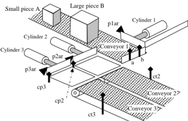
Conveyor 1 Conveyor 2 Conveyor 3 Cylinder 1 Cylinder 2 Cylinder 3
Small piece A Large piece B
ct2 ct3 cp3 cp2 p2ar p3ar p1ar a b
Fig. 2. Automated manufacturing system The sources are (Fig. 1):
- Operational information characterizing the desired behaviour (control model),
- Structural information coming from the process itself and the sensors-actuators spatial distribution (plant model),
- Temporal information coming from the reactivity of the actuators (temporal model).
The local diagnosers are based on the combination of the control, plant and temporal models. The goal is to diagnose all faults violating the desired behaviour. A minimal/maximal interval response times for each actuator is supposed to be known. Each local diagnoser is responsible of a specific part of the plant and uses event-based, state based and timed models to take a decision about fault’s occurrences. All local diagnosis decisions are then merged by a Boolean operator in order to obtain one global diagnosis decision.
To illustrate the proposed approach, we use the example of the figure 2 permitting the sorting of small and large pieces. It is composed of:
- One cylinder with three positions indicated by the sensors p1ar, cp2 and cp3. The cylinder moves forward upon the activation of the command
Out1 and the reverse action is obtained by the
command In1.
- Two cylinders are used to push the pieces onto their corresponding conveyor (conveyor 2 for small pieces and conveyor 3 for large pieces). These two conveyors are supposed to be in permanent rotation. Each cylinder has two sensors to indicate respectively its home and fully extended positions (p2ar and ct2 for the cylinder 2, p3ar and ct3 for the cylinder 3). The commands Out2 and Out3 are respectively for the activation of the forward movement for the cylinders 2 and 3. The two cylinders return back to their home position by the activation of respectively In2 and In3.
- The pieces are provided by the conveyor 1 which is activated by the command C1. This conveyor is in rotation until at least one of the detectors a and b has the logical value 1, due to the detection of a small piece (a = 1), a large piece (b = 1) or the fully extended position of the cylinder 1 (a or b = 1).
3. LOCAL DIAGNOSERS CONSTRUCTION
3.1 Plant model
The plant model construction is a complex operation. Firstly, a plant model is affected by combinatory explosion when a centralized approach is used. Secondly, all technology’s specificities must be expressed. To solve these problems, the plant is divided into several components (one for each actuator and its associated sensors) called Plant Element (PE). Consequently, the plant is composed
by n Plant Element: PEi, i ∈ {1, 2… n}. Each PEi is
modelled by an automaton Gi = (Xi, Σi, δi, xi0) with Xi
the set of states, Σi a set of finite events and it
includes the observable and unobservable events,
δi(σ, x) provides the set of possible next states if the
event σ occurs at state x and xi0 is the initial state.
Thus, the PE are defined as event-based model and use the Balemi interpretation (Balemi, et al., 1993)
where “↑” is the change of a value from 0 to 1 and
“↓”is the change of a value from 1 to 0. The detailed explication of the construction of this model can be found in (Philippot, 2006).
For the example of the figure 2, the plant is divided into 6 components: cylinders 1 with sensors p1ar,
cp2 and cp3, cylinder 2 with sensors p2ar and ct2,
cylinder 3 with sensors p3ar and ct3, conveyor 1 with sensors a and b, conveyor 2 with sensor ct2 and finally conveyor 3 with sensor ct3. We explain the construction of the plant model for the cylinder 2,
PEcy2. The plant models of the other components are
constructed in a similar way and can be found in
(Philippot, 2006). For PEcy2, there are 2 commands
producing 4 controllable events {↑Out2, ↓Out2,
↑In2, ↓In2} and 4 uncontrollable events
corresponding to the sensors outputs p2ar and ct2. The PEcy2 contains 15 states (Fig. 3).
3.2 Control model
The control model defines the global desired behaviour of the system and it is represented by the prefixed closed specification language K. Since the approach is decentralized, the control specification
must be locally integrated in each PEi to obtain a
Controlled Plant Element CPEi with i ∈ {1, 2… n}.
Each CPEi describes the local desired behaviour of
the component by an automaton Ci = (XCi, Σi, δi, xi0)
with a local specification language Ki = L(Ci).
Consequently, the desired behaviour language of a
CPEi is included in the language of the PEi (Ki ⊆
L(Gi)). 0 1 ↑Out2 ↓Out2 4 2 3 ↑In2 ↓In2 ↑In2 ↓In2 ↓In2 ↓Out2 ↑Out2 ↓Out2 ↑ct2 ↓p2ar ↓ct2 ↑p2ar 5 6 9 7 8 ↑In2 ↓In2 ↓In2 ↓Out2 ↑Out2 ↓Out2 10 11 14 12 13 ↑In2 ↓In2 ↓In2 ↓Out2 ↑Out2 ↓Out2 ↓p2ar ↑p2ar ↑ct2 ↓ct2 ↓p2ar ↑p2ar ↑ct2 ↓ct2 ↑Out2 ↓Out2 ↑In2 ↓In2 ↑Out2 ↓Out2 ↑In2 ↓In2
Fig. 3. Plant Element model PEcy2 of the cylinder 2
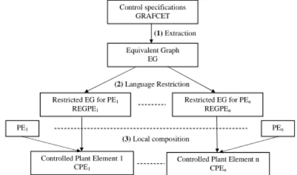
Control specifications GRAFCET PE1 Equivalent Graph EG PEn
Controlled Plant Element 1 CPE1
Controlled Plant Element n CPEn (1) Extraction (3) Local composition (2) Language Restriction Restricted EG for PE1 REGPE1 Restricted EG for PEn REGPEn
Fig. 4. Algorithm of intersection between Plant Element and Controller
The construction of the CPE is obtained by a local intersection between the PE and a global control model. GRAFCET is used to represent the global control model because it is widely used in industrial applications. However, GRAFCET semantics is different of the one of automata. Consequently, we have defined an algorithm to solve this problem, and it is based on the following three steps (Fig. 4): 1) The first step is the construction of an equivalent
automaton from the GRAFCET semantics. This automaton is obtained by an extraction algorithm described in (Philippot, 2006) and called Equivalent Graph (EG). The EG is constructed in function of the controllable and uncontrollable events of the system.
2) The restriction language for each PEi is done in the
second step. This restriction is obtained by an aggregation of states reached through non
observable events by the PEi. This aggregation
corresponds to a projection function or mask PL(Gi)(EG) of EG on the language L(Gi) of PEi
with the suppression of some states to guarantee the liveness of the model. This restriction is so-called Restricted Equivalent Graph for Plant
Element i (REGPEi) and is totally described in
(Philippot, 2006).
3) The third step is a local synchronized composition
between the REGPEi and the corresponding PEi.
The resulting automaton Ci of this composition
represents the local desired behaviour of the CPEi.
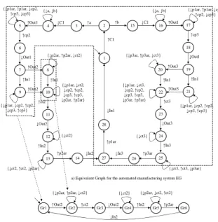
The global control model for the example of Fig. 2 is a GRAFCET with 8 steps and 9 transitions. The integration of the global control model locally in the plant model of the cylinder starts by the extraction of the Equivalent Graph EG of the GRAFCET (Fig. 5a). This EG is an automaton of 28 states.
The restriction language step of EG to the observable
events by PEcy2 gives a Restricted Equivalent Graph
for Plant Element of the cylinder 2 (REGPEcy2). This
latter is an automaton of 6 states where the state 1 is an aggregation of the states {1, 2, 3, 4, 5, 6, 7, 9, 15, 16, 17, 18, 19, 20, 21, 22, 23, 24, 25, 26, 27, 28} of the EG because there is non observable events by the
cylinder 2. It is the observable event ↑Out2 which
allows the transition to the state 2 (Fig. 5b). The controlled plant elements for the other components can be obtained in a similar way (Philippot, 2006).
{↓p1ar, ↑p1ar, ↓cp2, ↑cp2, ↓cp3} 2 ↑b 15 ↓C1 16 ↑Out1 1 ↑C1 14 26 ↑In1 5 ↑Out1 4 ↓C1 3 ↑a 20 ↑Out3 22 ↑Out3 ↑cp2 6 ↓In2 ↑p3ar ↑p2ar {↓a, ↓b} {↓p1ar, ↓cp2, ↑cp2, ↓cp3, ↑cp3} 17 ↓Out1 7 ↑In1 9 ↑cp3 18 ↓Out1 19 ↑In1 21 8 ↑Out2 10 ↑Out2 ↑In1 ↑ct2 11 ↓Out2 12 ↑In2 13 ↑ct3 23 ↓Out3 24 ↑In3 25 27 ↓In3 ↑p1ar 28 ↓In1 {↓a, ↓b} {↓p1ar, ↑p1ar, ↓cp2, ↑cp3, ↓cp3} {↓p3ar, ↑p3ar, ↓ct3} {↓p2ar, ↑p2ar, ↓ct2} {↓p1ar, ↓cp2, ↑cp2, ↓cp3, ↑cp3} {↓p1ar, ↓ct2, ↓cp2, ↑cp2, ↓cp3, ↑cp3, ↓p2ar, ↑p2ar} {↓p1ar, ↓ct3, ↓cp2, ↑cp2, ↓cp3, ↑cp3, ↓p3ar, ↑p3ar} {↓ct2, ↑ct2, ↓p2ar} {↓ct3, ↑ct3, ↓p3ar} {↓ct2} {↓ct3} Gr1 ↑Out2 Gr2 ↑ct2 Gr6 ↓In2
Gr3 ↓Out2 Gr4 ↑In2 Gr5 ↑p2ar {↓p2ar, ↑p2ar, ↓ct2} {↓ct2} {↓p2ar, ↓ct2, ↑ct2}
a) Equivalent Graph for the automated manufacturing system EG
b) Restricted Equivalent Graph for the Plant Element of the cylinder 2 REGPEcy2
Fig. 5. Language restriction for the cylinder 2
1 ↑Out2 2 ↓p2ar 6 ↑In2 5 ↓In2 3 ↑ct2 4 ↓Out2 8 ↑p2ar 7 ↓ct2
Fig. 6. Controlled Plant Element CPEcy2 of the
cylinder 2
The last step of the algorithm of intersection is the
local composition between the REGPEcy2 (Fig. 5b)
and the PEcy2 (Fig. 3). The desired behaviour of each
component leads to a Controlled Plant Element CPEi.
For the cylinder 2, the automaton CPEcy2 has 8 states
(Fig. 6).
3.3 Temporal information
The majority of sensors and actuators in manufacturing systems produces constrained events since state changes are usually effected by a predictable flow of materials (Boufaïed, 2003, Pandalai and Holloway, 2000). Therefore, a timed model centred on the notion of expected event sequencing and timing relationships can be used. The temporal information about events minimal and maximal occurrence instants is represented by the actuator’s minimal and maximal response times.
In this paper, we define a Prediction Function PFx
for each state x to evaluate the satisfaction, PFx = 0,
or the non satisfaction, PFx = 1, of the temporal
relationships between input and output events. Each prediction is constructed for observable correlated events and it describes the next events that should occur and the relative time periods in which they are expected. These pre-defined time periods are determined by experts according to the system dynamic and to the desired behaviour. This prediction has the following form: PFx1 = PF(α1, α2) = {α1, x1, (α2, [tmin1, tmax2], x2, l1)}. When the event α1
occurs at the state x1, the event α2 should happen at
the state x2 and within the interval [tmin1, tmax2]. If it is
the case then the prediction consequent is satisfied,
PFx1 = 0. When it is not the case, the event α2 has
occurred before tmin1 or after tmax2, the prediction
consequent is not satisfied and it provides the causes
of this non satisfaction through a decision function l1
corresponding to a faulty label (Fig. 7).
Prediction functions take into account the impression contained in the calculation of events occurrences instants. They also provide interesting information for the prediction of future failure, i.e., prognostic
(0<PFx<1). The value of the prediction function is
obtained by: ⎢ ⎢ ⎢ ⎢ ⎢ ⎢ ⎢ ⎢ ⎢ ⎣ ⎡ > ≤ < − ≤ ≤ < ≤ − < = Σ ∈ ∀ 2 max 2 max 1 max 1 max 2 max 1 max 1 max 2 min 2 min 1 min 2 min 1 min 2 min 1 min 2 1 2 1 if 1 if if 0 if if 1 ) , ( , , t t t t t t -t t t t t t t -t PF o τ τ τ τ τ τ τ α α α α
τ = θ(α2) - θ(α1) denotes the delay between the date θ(α1) of the event α1 and the date θ(α2) of the event
α2. Adding a prediction function at each state of each
CPEi leads to a new automaton called Temporized
Controlled Plant Element TCPEi with i ∈ {1, 2… n}.
For the Controlled Plant Element of the cylinder 2
CPEcy2, it is possible to establish all prediction
function for each state. The resulting automaton is called Temporized Controlled Plant Element for the
cylinder 2 (TCPEcy2) (Fig. 8). To understand this
automaton, let take as example the state x3 with the
prediction function PFx3 = PF(↓p2ar, ↑ct2) = {↓p2ar,
x3, (↑ct2, [5s, 15s], x4, F4)}. This function indicates that after the passage of the sensor p2ar to 0, the sensor ct2 must be equal to 1 after a delay belonging to the interval [5s, 15s] in order to reach the state x4. If the prediction function is not satisfied, a label F4 is returned to the user to indicate a fault. The other Temporized Controlled Plant Element can be obtained by the same manner (Philippot, 2006).
Prediction Function PF(α1, α2)
1 0
θ(α2) - θ(α1)
tmin1 tmin2 tmax1 tmax2
θ(α2) θ(α1) α2 α1 x1 PFx1(α1, α2) x0 PFx0(α0, α1) x2 PFx2(α2, α3) α0 α3
Fig. 7. Representation of a prediction function
x1 PFx1(↓In2,↑Out2) ↑Out2 ↓In2 ↓Out2 ↑In2 ↓p2ar ↑p2ar ↑ct2 ↓ct2 x2
PFx2(↑Out2,↓p2ar) PFx3(↓p2ar,↑ct2) x3 PFx4(↑ct2,↓Out2)x4
x8
PFx8(↑p2ar,↓In2) PFx7(↓ct2,↑p2ar) x7 PFx6(↑In2,↓ct2) x6 PFx5(↓Out2,↑In2) x5
Fig. 8. Temporized Controlled Plant Element TCPEcy2 of the cylinder 2
3.4 Local diagnosers
A local diagnoser Di is constructed and based on
each Temporized Controlled Plant Element (TCPEi).
This local diagnoser carries fault information by labels attached to states. These labels indicate the types of faults that have been occurred. Each local
diagnoser is considered as a Moore automaton: Di =
(Xi∪ XDFi, Σio, δi, xi0, Vi, hi, PFi, li) where: - Xi is the set of normal states of TCPEi,
- XDFi is the set of faulty states
- Σio is the set of observable events by PEi,
- δi : Xi × Σi* → Xi ∪ XDFi is the transition
function,
- xi0 is the initial state,
- Vi is an input/output vector with Vi(x) the vector
of the state x,
- hi : Xi∪ XDFi→ Σio is the output function where
hi(x) is the observable event at the output of the
state x,
- PFi = {PFx, ∀x ∈ Xi} represents the set of
prediction functions of a state x,
- li is the set of decision functions of the local
diagnoser Di with li(x) the decision function of
the state x which can be one or more fault labels {Fj}.
The local diagnoser uses a state-based model characterized by the input/output vector in each state. The dimension of this vector corresponds to the number of observable events of the local diagnoser
Di. In the state-based model, a fault is considered as
the consequence of reaching at some faulty states. Thus, it does not require to be initiated at the same time with the plant model.
For the local decision, if the label function at a state x
is li(x) = {N}, then the diagnoser, when it reaches the
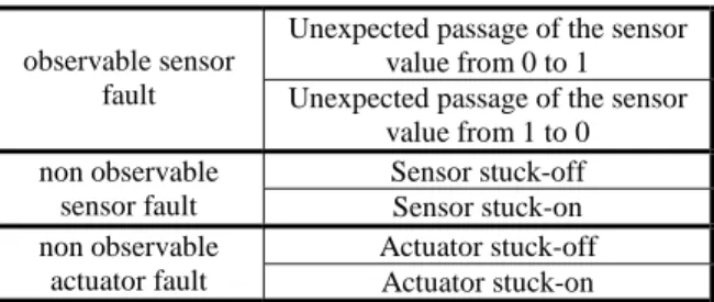
state x, can decide with certainty the non presence of faults. If the label function at a state x is li(x) = {Fj}, then the diagnoser indicates with certainty the occurrence of a fault of the type Fj. If li(x) contains the label N and any other fault label then the diagnoser, at a state x, cannot decide whether a fault has occurred or the system is in normal function, i.e., ambiguity or indecision case. To define the different labels, we have defined subsets of failures, each one is called fault partition. Then, each fault partition ΠFj is associated with a label Fj indicating the type of failures. We have considered two kinds of faults (Table 1): sensor’s faults and actuator’s faults. Failures can be modelled as observable or/and unobservable events.
Table 1 Possible faults on a Plant Element Unexpected passage of the sensor
value from 0 to 1 observable sensor
fault Unexpected passage of the sensor
value from 1 to 0 Sensor stuck-off non observable
sensor fault Sensor stuck-on
Actuator stuck-off non observable
actuator fault Actuator stuck-on
Table 2 Possible faults on the cylinder 2
f1 Unexpected passage of p2ar from 0 to 1
f2 Sensor p2ar stuck-off
f3 Unexpected passage of p2ar from 1 to 0
F1
f4 Sensor p2ar stuck-on
f5 Unexpected passage of ct2 from 0 to 1
f6 Sensor ct2 stuck-off
f7 Unexpected passage of ct2 from 1 to 0
F2
f8 Sensor ct2 stuck-on
f9 Cylinder 2 stuck-off
F3
f10 Cylinder 2 stuck-on
The case of observable events is a trivial one since failures can be detected as soon as they are. In the case of unobservable events, the occurrence of a failure must be inferred from the system model and future observations.
From each PEi, we can describe the set of
diagnosable faults of the process and define all the fault partitions. Each faulty state of the local diagnoser is obtained by an analysis of all possible faults than can be occurred from a normal state. From a normal state, it is possible to reach a faulty state: (i) for each unexpected passage of a sensor value, (ii) for a non observable fault of a sensor stuck or (iii) for a non observable fault of an actuator stuck (Philippot, 2006). From this, the outputs transitions from a normal to an abnormal state are represented by an
event fi which belongs to a fault partition of the local
diagnoser. The faults partitions for the cylinder 2 are defined in Table 2.
The local diagnoser Dcy2 for the cylinder 2, is
established based on TCPEcy2 and the set of all faults
which can be detected from each normal state. This diagnoser is an automaton of 24 states (8 normal states, 8 faulty states reached due to the occurrence of non observable faults and 8 faulty states reached due to the occurrence of observable faults).
Observable faults are directly diagnosed by an “Exclusive OR” operator between the input/output
vector Vi(x) of the current faulty state and the
estimated one (Philippot, 2006). If a non-expected event is generated, as an example the occurrence of
↑ct2 when the cylinder 2 is state x1, then the current state has an input/output vector Vcy2(x13) = (p2ar, ct2, Out2, In2) = (1100) whereas the one of the estimated
state, x2, is Vcy2(x2) = (1010). The comparison of this two vectors by an “Exclusive OR” operator allows detecting and isolating the observable failure in the sensor ct2: Vcy2(x13) ⊕ Vcy2(x2) = (0110). Indeed the value one in the resulting comparison is not equal to 0 and indicates a faulty element. The localisation of this faulty element is given by the last observable event.
Since the diagnosis of observable faults is trivial, the local diagnoser is simplified to take into account only
the non observable faults. The local diagnoser Dcy2 of
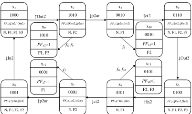
the cylinder 2 is presented in figure 9 (Philippot, 2006).
↑Out2 ↓In2 ↓Out2 ↑In2 ↓p2ar ↑p2ar ↑ct2 ↓ct2 1000 PFx1(↓In2,↑Out2) N, F1, F2, F3 1010 PFx2(↑Out2,↓p2ar) N, F2 0010 PFx3(↓p2ar,↑ct2) N, F1 0110 PFx4(↑ct2,↓Out2) N, F1, F2, F3 x8 1001 PFx8(↑p2ar,↓In2) N, F1, F2, F3 x7 0001 PFx7(↓ct2,↑p2ar) N, F2 x6 0101 PFx6(↑In2,↓ct2) N, F1 x5 0100 PFx5(↓Out2,↑In2) N, F1, F2, F3 x9 1010 PFx2=1 F1, F3 x10 0010 PFx3=1 F2 x12 0001 PFx7=1 F1 x11 0101 PFx6=1 F2, F3 f4, f9 f 6 f2 f8, f10
Fig. 9. Simplified diagnoser Dcy2 for the cylinder 2
3.5 Global decision
Each local diagnoser Di provides a Local diagnosis
Decision LDi corresponding to the label function lx at
the current state x of Di. Then, all local diagnosis
decisions are merged in order to obtain one Global diagnosis Decision (GD). This fusion is realized using an unconditional structure and based on a Boolean operator “Union”. If one local diagnoser announces a fault, then the global diagnosis decision will be this local decision. For the example of the figure 2, if the local diagnosis decisions of the
conveyor 1 is (LDC1), the cylinders 1 is (LDcy1), the
cylinder 2 is (LDcy2) and the cylinder 3 is (LDcy3),
then the global decision is obtained by: GD = LDC1
∪ LDcy1∪ LDcy2∪ LDcy3.
4. CONCLUSIONS
In this paper, a decentralized approach is proposed to diagnose manufacturing systems. This approach is based on several local diagnosers to detect and isolate the occurrence of each failure violating the system desired behaviour. This approach exploits all available information sources in order to construct a depth model of the system (plant, control, and actuator’s minimal and maximal response times). The local diagnosers are obtained by adding the faulty states, reached due to the occurrence of a failure. They are no need of communication between local diagnosers because this approach uses event-based, state based and timed models to take a decision about fault’s occurrences. Consequently, there is no propagation of local faults. Each diagnoser detects faults with earliest to send it local decision which will be merged with the others for a global decision.
To determine if the system can be diagnosed according to its observable events and for the set of defined failures, which can be observable or non observable, an adapted codiagnosability notion has been defined in (Philippot, 2006). This is a timed-event-based codiagnosability notion. In this work, a
simulation tool based on Stateflow of Matlab® has
been constructed to test and validate the proposed approach.
One drawback of the approach is the fact that only the equipments, actuators and sensors, faults are
conveyors. To solve this drawback, a solution is to construct a model representing the parts normal and faulty behaviours by using Colored Petri Nets. CPN use the colour in generics models. Consequently, it is not necessary to make a model for each part to follow-up. Another drawback is that this approach was not tested on real applications. One solution is to develop the simulation tool to be applied for the on-line implementation as an OPC (OLE for Process Control) client. Consequently, a connexion to an
OPC server from Matlab® allows reaching the
Programmable Logic Controller (PLC) variables.
REFERENCES
Balemi, S., G.J. Hoffmann, P. Gyugyi, H. Wong-Toi, G.F. Franklin (1993). Supervisory control of a rapid thermal multiprocessor. In: IEEE
Transactions on Automatic Control, Vol. 38,
n°7, pp.1040-105.
Boufaïed, A. (2003). Contribution à la Surveillance Distribuée Des Systèmes à Evénements Discrets Complexes. In: Thesis of PhD,Université Paul
Sabatier, Toulouse.
Cassandras, C.G., S. Lafortune (1999). Introduction to Discrete Event Systems. In: Kluwer
Academic, Publisher.
Darkhovski, B., M. Staroswiecki (2003). A Game-Theoretic Approach to Decision in FDI. In:
IEEE Transactions On Automatic Control,
Vol.48, n°5.
Debouk, R., S. Lafortune, D. Teneketzis (2000). Coordinated decentralized protocols for failure diagnosis of discrete event systems. In: Discrete
Event Dynamic Systems: Theory and Applications, Vol. 10, n°1-2, pp.33-86.
Genc, S., S. Lafortune (2003). Distributed diagnosis of discrete-event systems using Petri nets. In:
International Conference on Application and Theory of Petri Nets, pp.316-336, Eindhoven,
The Netherlands.
Klein, S., L. Litz, J.J. Lesage (2005). Fault Detection of Discrete Event Systems Using an Identification Approach. In: 16th IFAC World
Congress, CDRom paper n°02643, Praha (CZ).
Pandalai, D., L.E.N. Holloway (2000). Template Languages for Fault Monitoring of Timed Discrete Event Processes. In: IEEE Transactions
On Automatic Control, Vol. 45, n°5.
Philippot, A. (2006). Contribution au diagnostic décentralisé des Systèmes à Evénements
Discrets : Application aux systèmes
manufacturiers. In: Thesis of PhD, Université de
Reims Champagne Ardenne.
Wang, Y. T. Yoo, S. Lafortune (2004). New results on decentralized diagnosis of Discrete Event
Systems. Allerton Conferences
Urbana-champaign, IL, USA.
View publication stats View publication stats