HAL Id: hal-01714844
https://hal.archives-ouvertes.fr/hal-01714844
Submitted on 23 Feb 2018
HAL is a multi-disciplinary open access
archive for the deposit and dissemination of
sci-entific research documents, whether they are
pub-lished or not. The documents may come from
teaching and research institutions in France or
abroad, or from public or private research centers.
L’archive ouverte pluridisciplinaire HAL, est
destinée au dépôt et à la diffusion de documents
scientifiques de niveau recherche, publiés ou non,
émanant des établissements d’enseignement et de
recherche français ou étrangers, des laboratoires
publics ou privés.
Obstacle Avoidance Controller Generating Attainable
Set-points for the Navigation of Multi-Robot System
Ahmed Benzerrouk, Lounis Adouane, Philippe Martinet
To cite this version:
Ahmed Benzerrouk, Lounis Adouane, Philippe Martinet. Obstacle Avoidance Controller Generating
Attainable Set-points for the Navigation of Multi-Robot System. IEEE Intelligent Vehicles Symposium
(IV), Jun 2013, Gold Coast, Australia. �hal-01714844�
Obstacle Avoidance Controller Generating Attainable Set-points for the
Navigation of Multi-Robot System
A. Benzerrouk
1, L. Adouane
1and P. Martinet
21 Clermont Université, Université Blaise Pascal, BP 10448, 63000 Clermont-Ferrand, France
2 IRCCYN, Ecole Centrale de Nantes, 1 rue de la Noé,
BP 92101, 44321 Nantes Cedex 03, France
Abstract— This paper considers the navigation in formation of a mobile Multi-Robot System (MRS) in presence of obstacles. In such areas, the collision avoidance between the robots themselves and with other obstacles (static and dynamic) is a challenging issue. To deal with it, a reactive and a distributed control architecture is built. The navigation in formation of the MRS is ensured while tracking a global virtual structure (first controller). Limit-cycle principle is used to compute the set-point of the obstacle avoidance task (second controller). In this paper, kinematic constraints of the robot are taken into account in order to generate an attainable set-point. The objective is to guarantee safety of the mobile robots with respect to their maximum velocities. Simulation and experimental results validate the proposed contributions.
I. INTRODUCTION
Navigation of multiple mobile robots is a recurrent re-search subject due to a large amount of the met issues. Safety of the robots in cluttered environment is among the most important ones. Collision avoidance is then widely investigated in the literature for multi-robot systems. It is tackled through two main approaches. The first one considers the robots control entirely based on path planning methods, which involve the prior knowledge of the robots environment. The objective is to find the best path to all the robots in order to avoid all the obstacles and each other while minimizing a cost function [1], [2]. This first method requires a significant computational complexity, especially when the environment is highly dynamic. In fact, the robot has to frequently replan its path.
Rather than a prior knowledge of the environment, reactive methods are based on local robots sensors information. At each sample time, robot’s control is computed according to its perceived environment. Potential field [3] and the Deformable Virtual Zone (DVZ) [4] are a good illustration of reactive approaches. The reactive methods given above suffer from local minima problems when, for instance, the sum of potential forces is null, or the deformation of the DVZ is symmetric (as in the U shape obstacle case). Gen-erally, reactive methods do not require high computational complexities, since robots actions must be given in real-time according to the perception.
The distributed architecture of control, that we developed [5], deals with this last kind of methods. The studied task is the navigation in formation. The formation is considered
as a virtual structure (rigid body) and the control law for each robot is derived by defining the dynamics of this body. Virtual structure approach is often associated to potential field applications since they are simple and allow collision avoidance [6], [7]. However, potential forces are limited, especially when the formation shape needs to be frequently reconfigured. In fact, it means that the robot is submitted to a frequently-changing number/amplitude of forces leading to more local minima, oscillations, etc. Hence, it was proposed that the robots track a virtual body without using potential forces. Since collision avoidance must stay possible despite the absence of potential fields, behavior-based concept [8], [9] was introduced. This allows to divide the task into two different behaviors (controllers): Attraction to Dynamic
Target, and Obstacle Avoidance (cf. Figure 1). The latter was
based on limit-cycle differential equations [10]. Limit-cycle navigation was already used for obstacle avoidance [11], [12]. It allows to choose the obstacle avoidance direction (clockwise or counterclockwise) in order to rapidly join the assigned target. In [13], it is proposed to extend this method to dynamic obstacles and to robots of the same system without loosing the control reactivity. Unlike most of algorithms addressing dynamic obstacles, no communication is required among the robots to accomplish the task. Avoid-ance is based only on the local perception of each robot. As in [11], [12], the idea is to find the best direction of avoidance. It was proved that only the velocity vector of the obstacle is sufficient to deduce this direction. In this paper, our architecture is enriched by constraining the set-point generated by obstacle avoidance controller: this set-point has to be attainable despite the maximum velocities of the robot and dimensions of the obstacles in order to guarantee the robot’s safety. New parameters are then introduced to the set-point formula to prevent the robot from collision.
The remainder of the paper is organized as follows. Section II gives the principle of the navigation in formation and the general control architecture. Basic controllers and the control law are reminded in this section. In section III, the set-point generated by obstacle avoidance is modified to deal with each robot according to its maximum velocity and to the obstacle dimensions. Section IV validates the proposed contribution with experimental results. Finally, we conclude and give some perspectives in section V.
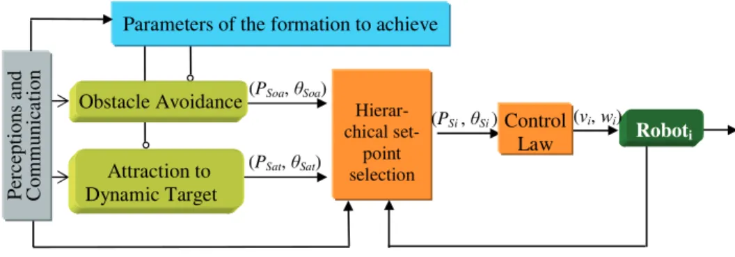
Hierar- chical set-point selection Attraction to Dynamic Target Roboti (PSoa, Soa) (PSi , Si ) Control Law (vi, wi) P erc ept ions a nd C o m m u n ic at io n Obstacle Avoidance
Parameters of the formation to achieve
(PSat, Sat)
Fig. 1. The proposed architecture of control embedded in each robot.
II. CONTROLARCHITECTURE
The used control architecture includes two controllers:
Attraction to Dynamic Target and Obstacle Avoidance. The
virtual structure is built through the Parameters of the
Formation to Achieve block (cf. Figure 1).
According to environment information collected by the
Perceptions and Communication block (sensors) and the
robot’s current state, one controller is chosen thanks to the
Hierarchical Set-Point Selection block.
The corresponding set-points(PSi, θSi) (position and ori-entation) are then sent to the Control Law block which calculates the linear and angular velocities noted vi and wi
respectively (cf. Figure 1).
A. Parameters of the Formation to Achieve block
This subsection briefly describes the adopted virtual
struc-ture principle. Consider N robots with the objective of
reaching and maintaining them in a given formation. The proposed virtual structure that must be followed by the group of robots is defined as follow:
• Define one point which is called the main dynamic
target (cf. Figure 2),
• Define the virtual structure to follow by defining NT
nodes (virtual targets) to obtain the desired geometry. Each nodei is called a secondary target and is defined
according to a specific distance Di and angleΦi with respect to the main target. The number of these targets
NT must beNT ≥ N .
Each roboti has to track a predefined target i. An exemple
to get a triangular formation is given in figure 2.
B. Attraction to Dynamic Target controller
To remind the Attraction to Dynamic Target controller which allows to reach and to keep the formation, consider a robot i with (xi, yi, θi) pose. This robot has to track
its secondary dynamic target. To simplify notations in the following, the same subscript of the robot is given to its target. The latter is then notedTi(xTi, yTi, θT) (cf. Figure 3) and the variation of its position can be described by
( ˙xTi= vTi.cos(θT) ˙yTi = vTi.sin(θT) (1) Di Dj j T Ow Xw Yw Main dynamical target Secondary target vT Dk k i Robotq Robotp Robotr
Fig. 2. Keeping a triangular formation by defining a virtual geometrical
structure. i Ym Xm Om(xi , yi) dSi Ow Xw Yw i T vTi Ti (xTi , yTi ) Secondary Virtual Target
Fig. 3. Attraction to Dynamic Target.
Let’s also introduce the used robot model (cf. Figure 3). Experimental results are made on Khepera robots, which are unicycle mobile robots. Their kinematic model can be described by the well-known equations (cf. Equation 2).
˙xi= vi.cos(θi) ˙yi= vi.sin(θi) ˙ θi= ωi (2)
whereθi, vi andωi are respectively the robot orientation, the linear and angular velocities.
The set-point angle that the robot must follow, to reach its dynamic target, is given by
θSati = arcsin(b sin(θT − γi)) + γi (3) Whereb = vTi
vi .γi is the angle that the robot would have if it was directed to its target (cf. Figure 3). This set-point
has been obtained by keepingγi constant. More details and proofs are available in [5].
The corresponding set-points (PSi, θSi) (cf. Figure 1) given by the Attraction to Dynamic Target controller are composed by:
• (PSi= (xTi, yTi)): the current position of the dynamic target (cf. Figure 3),
• (θSi = θSati) given by equation (3).
C. Obstacle Avoidance controller
A particular attention is given to this controller since the objective of the paper is to make its set-point attainable despite the kinematic constraints of the robots. As cited in section I, the task is performed through the limit cycle methods. The robot follows the limit cycle vector fields described by the following differential equations:
˙xs = (sign)ys+ µxs(R2
c− x2s− ys2) ˙ys = −(sign)xs+ µys(R2
c− x2s− y2s)
(4) where (xs, ys) corresponds to the relative position of the robot according to the center of the convergence circle (characterized by anRc radius).
The function sign allows to define the direction of the
trajectories described by these equations. Hence, two cases are possible:
• sign = 1, the motion is clockwise.
• sign = −1, the motion is counterclockwise.
Figure 4 shows the limit cycles with a radius Rc = 1.
The Obstacle is then covered by a circle, which is itself surrounded by an other virtual circle of influence with Rc
radius (cf. Figure 6). The latter is chosen as the sum of the obstacle radius, the robot radius and a safety margin. µ is
a positive constant. Figure 5 illustrates its influence on the limit-cycle trajectory. The choice of this constant will be rigorously discussed in section III to generate an attainable set-point.
The set-point angle θSoa of the Obstacle Avoidance con-troller is given by the following relation
θSoa= arctan(
˙ys
˙xs) (5)
The corresponding set-points(PSi, θSi), -when the
Obsta-cle Avoidance controller is chosen by Hierarchical Set-Point Selection block (cf. Figure 1)-, are defined such that
• (PSoa= (xo, yo)) corresponds to the center position of the obstacle, -3 -2 -1 0 1 2 3 -3 -2 -1 0 1 2 3 x s ys (a) Clockwise (sign = 1) -3 -2 -1 0 1 2 3 -3 -2 -1 0 1 2 3 x s ys (b) Counter-Clockwise (sign = −1)
Fig. 4. Possible trajectories of the limit-cycles
µ=2
µ = 4
µ=3
µ=1
µ=0.5
Fig. 5. Influence of µ on the limit-cycle trajectory smoothness.
• (θS= θSoa).
It is noticed that previous works on limit-cycle methods applied to obstacle avoidance [11], [12] do not consider dynamic obstacles. Here, it is proposed to extend this reactive method to deal with them.
According to the nature of the obstacle, three cases are considered: static obstacles, dynamic obstacles, and robots of the same system. These strategies are briefly reminded in the next paragraphs. More details are available in [13].
1) static obstacles, 2) dynamic obstacles, 3) robots of the same system.
1) Static obstacles: The same strategy proposed in [12]
is maintained. Summarily, the value ofsign is specified by
the ordinate of the robotys in the relative obstacle’s frame
(OoXoYo) (cf. Figure 6). The Xo axis of this orthonormal frame is defined thanks to two points: the center of the obstacle (which makes the origin of the frame) and the target to reach. sign= ( 1 ifys≥ 0 (clockwise avoidance) −1 ifys< 0 (counterclockwise avoidance) (6) The chosen direction by this strategy allows then to join the target by the side offering the smallest covered distance.
ys >0 vOx obstacle Target Robot YO O X Ow Xw Yw Oi α vO vOy Circle of influence
Fig. 6. Avoiding an obstacle. Static obstacle: the ordinate ysis analyzed,
dynamic one: projection of ~vO is analyzed.
2) Dynamic obstacles: Rather than analyzing the sign of ys, it is proposed that the robot uses the obstacle’s vector velocity~vO. The idea is to project this vector on theYoaxis of the relative frame(OoXoYo) defined in paragraph II-C.1.
The functionsign (cf. Equation 4) is then defined
accord-ing tovOy as follows: sign= ( 1 ifvOy ≤ 0 (clockwise avoidance) −1 ifvOy > 0 (counterclockwise avoidance) (7)
By using the projection vOy of the obstacle velocity, the obstacle is always avoided round the back, such that the robot never cuts off the obstacle’s trajectory.
3) Robots of the same system: One can consider that
every robot of the MRS is treated as a dynamic obstacle and projects its velocity vector to deduce the side of avoidance (cf. Equation 7). However, a conflict problem could appear when, for instance, two robots have to avoid each other in opposite directions calculated by velocity vector projections. To deal with this kind of conflicts, and assuming that each robot is able to identify those of the same system, it is proposed to impose one reference direction for all the system. Hence, when one robot detects a disturbing robot of the same group, it always avoids it counterclockwise.
D. The control law block
This block allows for the robot i to converge to its
set-point given by the Hierarchical set-set-point selection block (cf. Figure 1). It is expressed as
vi= vmax− (vmax− vT)e−(d2Si/σ2) (8a) ωi= ωSi+ k ˜θi (8b) where
• vmax is the maximum linear speed of the robot, • σ, k are positive constants,
• vi andωiare linear and angular velocities of the robot. ωSi= ˙θSi,
• and ˜θi= θSi− θi is the error orientation.
θSi is the set-point angle according to the active controller (cf. Equation (3), (5)). Asymptotic stability of the control law is demonstrated in [13]. In fact, it can be easily deduced from equation (8b) that the error orientation exponentially converges.
It is also noticed that linear velocity vi is made so that
vi≤ vmax is always verified. Naturally, for target following case, it is imposed thatvT < vmaxto attain the virtual target. Next section, the main contribution of this paper, prevents saturation of the angular velocity from occurring despite the robot’s kinematic constraints.
III. OBSTACLE AVOIDANCE WITH RESPECT TO
KINEMATIC ROBOT CONSTRAINTS
Now, we are interested in the maximum angular velocity of the robots ωmax, such that the variation of the angular set-point ˙θSoai remains attainable (i for the i
th robot) and
safety of the robot guaranteed. As previously explained, we are interested in the obstacle avoidance case. Attraction to
Dynamic Target study is subject of a future paper.
It is clear that the angular velocity applied to the robot has to verify
|ωi| ≤ ωmax (9)
whereωmax> 0. By replacing (8b) in (9), we have ωSi+ k ˜θi ≤ ωmax (10) knowing that ωSi+ k ˜θi ≤ |ωSi| + k ˜ θi
To find the values ofωSi which verify (10), it is proposed to use |ωSi| + k θi˜ ≤ ωmax (11)
To be always verified, the latter relation then becomes
|ωSi| ≤ min |θ˜i|(ωmax− k θi˜ ) (12) Which leads to |ωSi| ≤ (ωmax− k max θi˜ ) (13)
Since the proposed control law is asymptotically stable (cf. Section II-D), and the orientation error is exponentially decreasing, the following relation is easily deduced
max θi˜ = θi(ts)˜ (14)
wheretsis the switching moment to the Obstacle
Avoid-ance controller.
Since ωSi = ˙θSoai, let us compute ˙θSoai according to equation (5) ˙θSoa = d dt( ˙ ys ˙ xs) (1+(ys˙ ˙ xs) 2) (15) To develop ˙θSoa, we note A = R2c− x2s− ys2 (16)
Using equation (4), (15) leads to
˙θSoa= −sign − 2signµ 2A(x2 s+ y2s)/(sign2+ µ2A2) (17) Replacing in (13), we obtain 1 + 2µ 2A (x2s+ y2s) (1 + µ2A2) ≤ ωmax− k θi(ts)˜ (18)
We can use the following relation
1 + 2µ2A (x 2 s+ y2s) (1 + µ2A2) ≤ ωmax− k θi(ts)˜ (19)
In fact, values ofµ verifying (19), verify also (18).
On the other side, it is clear that (cf. Equation 18)
0 ≤ 2µ2A (x2s+ y2s) (1 + µ2A2) ≤ ωmax− k ˜ θi(ts) − 1 (20)
The gaink has then to verify ωmax− k
θi(ts)˜
− 1 > 0 (21)
and the allowed values ofk are k < ωmax − 1 ˜ θi(ts) (22)
To deal with the worst possible configurations,k is chosen
such that
k < ωmax− 1
π (23)
In fact, the maximum value of ˜ θi(ts)
= π, since the
maximal possible orientation error corresponds to the case where the robot orientation is in the opposite of the set-point angle.
The left member of the inequation (18) can be bounded as follows 1 + 2µ2A (x 2 s+ ys2) (1 + µ2A2) ≤ 1 + 2µ2A(x2s+ ys2) (24)
In fact, using the right member of (24) is simpler to find values ofµ verifying the condition (20). Hence, to find these
values, the following relation is used
2µ2|A| (x2s+ ys2) ≤ ωmax− k θi(ts)˜ − 1 (25)
In what follows, we note Poa = ωmax− k
θi(ts)˜ − 1.
To always generate a reachable set-point angle ˙θSoa of the obstacle avoidance controller,µ has then to be chosen as
µ2≤ Poa 2 |A| (x2
s+ ys2)
(26) The distance of the robot to the obstacle noteddROcan be introduced to the last relation (26) which becomes (replacing
A defined in (16))
µ2≤ Poa
2 |R2
c− d2RO| d2RO
(27) To find a least upper bound ofµ regardless of dRO, it is proposed to compute the minimum of the right member of (27) (which corresponds to the maximum of its denomina-tor). When the obstacle avoidance is activated, two cases can be distinguished :
1) dRO < Rc (the robot is inside the limit-cycle) this gives
Den = (R2c− d2RO)d2RO
Its derivative with respect todRO is
∂Den
∂dRO = 2dRO(R 2
c − 2d2RO) (28)
Roots corresponding to the maximum of Den are
±R√c
2. (the solutiondRO= 0 is rejected since it means
that the distance between the robot and the obstacle centers is null, which is impossible). Replacing in (27),
µ has to satisfy
µ ≤ 1 R2
c
p2Poa (29)
2) dRO > Rc (the robot is outside the limit-cycle)Den
becomes Den = −(R2c− d2RO)d2RO its derivative is ∂Den ∂dRO = −2dRO(R 2 c− 2d2RO)
There is no solution satisfying the conditiondRO > Rc
(the Den domain of definition corresponding to the
second case). In addition, Den is always increasing
and max(Den) is attained when dRO → ∞. In
practice, the robot is continuously approaching the obstacle (the robot is outside the limit-cycle in this
case) and the maximum considered distance dRO can
be chosen when the obstacle avoidance controller is activated. It is noteddRO0.
µ must then satisfy the following condition µ ≤ s Poa 2 R2c− d2RO 0 d2RO 0 (30) Finally, note that the case wheredRO = Rc means that the robot is on the limit-cycle. According to relation (27), any value ofµ can then be accepted. In fact, figure 5 shows that µ does not affect the trajectory smoothness on the limit-cycle
but only when converging to it.
Next section illustrates how the choice of µ directly
influences the safety of the robots.
IV. SIMULATION AND EXPERIMENTAL RESULTS
A. Simulation results
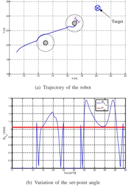
It is proposed to show how the proposed bound of the parameter µ constrains the set-point angle ˙θSoa and then guarantees a safe navigation. A mobile robot going toward a static target(vT = 0) in presence of obstacles is simulated.
We set ωmax = 3rd/s, and k = 0.6 (cf. Equation 23).
First, the simulation is accomplished using(µ = 1) which
assumes that the classic equations of limit-cycles are used (cf. Equation 4) (withoutµ). Figure 7(a) shows that the robot
avoids the first obstacle but fails to avoid the second one. Figure 7(b) shows the variation of the set-point angle ˙θSoa: it increases and becomes higher than the authorized value
Poa imposed by the maximum angular velocity of the robot
ωmax. It means that the robot’s dynamic can not follow this variation and then may collide with the obstacle.
8 10 12 14 16 18 20 22 24 16 18 20 22 24 26 1 2 X [m] Y [ m ] Target
(a) Trajectory of the robot
0 5 10 15 20 25 30 35 40 45 50 55 0 0.2 0.4 0.6 0.8 1 1.2 1.4 1.6 1.8 Temps[s/10] | θSoa | [r d /s ] |θS oa | P oa . . Time
(b) Variation of the set-point angle
Fig. 7. A mobile robot avoiding two obstacles (constant µ = 1).
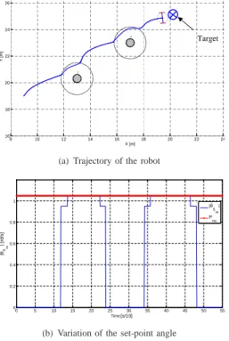
Now, simulation is run again in the same environment (position and dimension of the obstacles, initial conditions of the robot) by replacingµ with its constrained value (cf.
Equation 30) (the robot is outside the obstacles). It is noticed that this time, the robot succeeds to avoid the two obstacles (cf. Figure 8). The variation of the set-point can not exceed
Poa thanks to a re-computedµ (cf. Figure 8).
8 10 12 14 16 18 20 22 24 16 18 20 22 24 26 1 2 X [m] Y [ m ] Target
(a) Trajectory of the robot
0 5 10 15 20 25 30 35 40 45 50 55 0 0.2 0.4 0.6 0.8 1 Temps[s/10] | θS oa | [r d /s ] |θ Soa | P oa . . Time
(b) Variation of the set-point angle
Fig. 8. Dynamic of the mobile robot avoiding two obstacles (µ recomputed for each one).
B. Attaining a formation while avoiding collision between the robots
Experimentations are made on Khepera III robots and illustrate a navigation in formation of the robots while avoiding each other. A central camera, at the top of the platform gives positions of all the robots and the obstacles thanks to circular bar codes installed on them. The objective, in short term horizon, is to use the local sensors of the robots in order to get a completely decentralized architecture.
The scenario illustrates three robots which have to join a triangular virtual structure. The latter moves along a circular trajectory (cf. Figure 9). Robots are put in their initial conditions so that they must avoid each other before joining the formation. It is observed that the collision avoidance is successfully accomplished for all the robots. Moreover, no conflict was observed since avoidance is done in one direction (robots of the same system)(cf. Section II-C.3). The formation is attained as shown in figure 9 illustrating the trajectories of the three robots.
V. CONCLUSION
The proposed control architecture devoted to the naviga-tion in formanaviga-tion in presence of obstacles must be enriched to generate only attainable set-points. In fact, the proposed control law is theoretically stable. However, in practice, additional constraints must be taken into account. In our case, kinematic constraints (maximum velocities) of the robot imposes to define maximum authorized set-points. It is then proposed to study the obstacle avoidance controller case.
Trajectory of the virtual structure along the circle R3 (t1) R2 (t1) R1 (t1) R1 (t2) R2 (t2) R3 (t2) Virtual structure at moment t0
Fig. 9. Trajectories of the robots attaining the formation.
Usually, its set-point depends on the obstacle characteris-tics (dimensions, shape, etc.). These parameters depends on the environment and can not be directly modified. A new parameter is then added to adapt the set-point according to these characteristics. Saturation of the velocities are avoided while ensuring safety of the robot. Future works will tackle the Attraction to Dynamic Target controller constraints. The objective is to define the allowed dynamic of the virtual structure to stay attainable.
REFERENCES
[1] S. J. Guy, J. Chhugani, C. Kim, N. Satish, M. Lin, D. Manocha, and P. Dubey. Clearpath: Highly parallel collision avoidance for multi-agent simulation. In ACM SIGGRAPH Eurographics symposium on
computer animation, 2009.
[2] A. Pongpunwattana and R. Rysdyk. Real-time planning for multiple autonomous vehicles in dynamic uncertain environments. Journal of
Aerospace Computing, Information and Communication, 1:580–604,
2004.
[3] O. Khatib. Real time obstacle avoidance for manipulators and mobile robots. International Journal of Robotics Research, 5:90–99, 1986. [4] R. Zapata and P. Lepinay. Reactive behaviors of fast mobile robots.
Journal of Robotics Systems, 11:13–20, 1994.
[5] A. Benzerrouk, L. Adouane, L. Lequievre, and P. Martinet. Navigation of multi-robot formation in unstructured environment using dynamical virtual structures. IEEE/RSJ International Conference on Intelligent
Robots and Systems, 2010.
[6] P. Ogren, E. Fiorelli, and Leonard N. E. Formations with a mission: Stable coordination of vehicle group maneuvers. In 15th International
Symposium on Mathematical Theory of Networks and Systems, 2002.
[7] K. D. Do. Formation tracking control of unicycle-type mobile robots. In IEEE International Conference on Robotics and Automation, pages 527–538, 2007.
[8] T. Balch and R.C. Arkin. Behavior-based formation control for multi-robot teams. IEEE Transactions on Robotics and Autmation, 1999. [9] G. Antonelli, F. Arrichiello, and S. Chiaverini. The nsb control: a
behavior-based approach for multi-robot systems. PALADYN Journal
of Behavioral Robotics, 1:48–56, 2010.
[10] H.K. Khalil. Frequency domain analysis of feedback systems (chapter
7). 2002.
[11] D. Kim and J. Kim. A real-time limit-cycle navigation method for fast mobile robots and its application to robot soccer. Robotics and
Autonomous Systems, 42:17–30, 2003.
[12] L. Adouane. Orbital obstacle avoidance algorithm for reliable and on-line mobile robot navigation. In 9th Conference on Autonomous
Robot Systems and Competitions, May 2009.
[13] A. Benzerrouk, L. Adouane, and P. Martinet. Dynamic obstacle
avoidance strategies using limit cycle for the navigation of multi-robot system. 4th Workshop on Planning, Perception and Navigation for