Measurements of Vertically Polarized Electromagnetic Surface Waves Over a Calm Sea in HF Band. Comparison to Planar Earth Theories

HAL Id: hal-01114356

https://hal.archives-ouvertes.fr/hal-01114356

Submitted on 9 Feb 2015

HAL is a multi-disciplinary open access

archive for the deposit and dissemination of

sci-entific research documents, whether they are

pub-lished or not. The documents may come from

L’archive ouverte pluridisciplinaire HAL, est

destinée au dépôt et à la diffusion de documents

scientifiques de niveau recherche, publiés ou non,

émanant des établissements d’enseignement et de

Measurements of Vertically Polarized Electromagnetic

Surface Waves Over a Calm Sea in HF Band.

Comparison to Planar Earth Theories

Mathilde Bellec, Stéphane Avrillon, Pierre Yves Jezequel, Sébastien Palud,

Franck Colombel, Philippe Pouliguen

To cite this version:

Mathilde Bellec, Stéphane Avrillon, Pierre Yves Jezequel, Sébastien Palud, Franck Colombel, et al..

Measurements of Vertically Polarized Electromagnetic Surface Waves Over a Calm Sea in HF Band.

Comparison to Planar Earth Theories. IEEE Transactions on Antennas and Propagation, Institute

of Electrical and Electronics Engineers, 2014, 62, pp.3823 - 3828. �10.1109/TAP.2014.2317493�.

�hal-01114356�

Measurements of Vertically Polarized

Electromagnetic Surface Waves Over a Calm Sea

in HF Band. Comparison to Planar Earth Theories.

Abstract—Radio communication over Earth along mixed-paths in the HF

band is a relevant subject today. In this paper, we present measurements of electric field propagating over sea water in HF Band compared to K.A. Norton, R.W.P. King and G. Millington’s theories, thanks to a reliable measurement setup. The transmitting antennas are located on the coast while the receiver antenna is installed on a boat steering a constant course. The electric field measurements are carried out with a loop antenna and we measured the field strength attenuation versus distance between the transmitter and the boat along a sea water path. In order to take into account the media change (the coast and the sea water), Millington’s solution has been added to King’s and Norton’s theories with the planar Earth model. The measurements performed at three frequencies (10 MHz, 20 MHz and 30 MHz) and the calculations are in a good agreement. At 10 MHz, the “smoothly” attenuation is shown and is very well correlated with the theory. The EM field decrease as 1/d² has been clearly observed at 20 MHz and 30 MHz.

Keywords— HF band measurements, surface-wave propagation, ground-wave field, vertical electric dipole, planar Earth model.

I. INTRODUCTION

Introduced at the beginning of the last century, surface-wave propagation has been largely investigated starting by Sommerfeld [1]

and followed by Norton [2], [3], King [4]-[6], Wait [7], [8]. These pioneer researchers provided mainly theoretical studies and analytical solutions to this problem. Sommerfeld started by calculating the EM field radiated by an infinitesimal vertical electric dipole located on the surface of the planar Earth. Then, Norton introduced the attenuation function, the ground effect, and the frequency dependence of the surface wave radiated by a vertical dipole. Based on Maxwell’s equations, R.W.P. King established the EM field expression generated by a vertical electric dipole located on or in the vicinity of the surface of a planar Earth and described the surface-wave propagation behavior. King also introduced characteristic distances to explain the attenuation factor variation along the path. In order to model mixed-path surface wave propagation effects, Millington [9], [10] developed an analytical method which takes into account the ground characteristics changes along the path. Recently, L. Sevgi [11]-[13] has developed significant contributions which integrate surface-waves propagation along mixed-path. All these studies are mainly theoretical and the measurements are unusual.

This work was supported in part by TDF and the “Direction Générale de l’Armement”.

M. Bellec, S. Avrillon and F. Colombel are with the institute of Electronics and Telecommunication of Rennes (IETR), UMR CNRS 6164, University of Rennes 1, Campus de Beaulieu, Rennes Cedex 35042, France.

(e-mail: mathilde.bellec@tdf.fr; stephane.avrillon@univ-rennes1.fr; franck.colombel@univ-rennes1.fr)

S. Palud and P-Y Jezequel are with TDF, La Haute

Galesnais, Centre Mesure d'Antennes, 35340 Liffré, France. (e-mail : sebastien.palud@tdf.fr; pierre-yves.jezequel@tdf.fr)

Ph. Pouliguen is with the « Direction Générale de l’armement » (DGA), DGA-DS/MRIS, 7-9, rue des Mathurins, Bagneux Cedex 92221, France (e-mail : philippe.pouliguen@intradef.gouv.fr)

This propagation phenomenon should present attractive and useful features for industrial applications because the surface waves propagate along the surface of Earth and beyond the radio-electric horizon. Few examples already exist mainly operating in VLF, LF and in the HF band. Thanks to these properties, the surface waves allow communication in hard environments (forest…) or target detection at very low elevation and at large distances.

This paper presents the measurements of surface waves over the sea in HF band and gives the comparison between the experimental studies and the theoretical models provided in the literature, especially in order to validate the surface wave decrease as 1/d and 1/d² along the path, and the characteristic distances introduced by King.

Section II presents the surface-wave propagation theories proposed by Norton, King, and Millington where the radiating element is a vertically polarized antenna located above the ground. Section III presents measurements realized over the sea. The measurement process is carefully described including the design of the antennas used to radiate the surface waves. Then, section IV provides a comparison between the measurements and the theoretical results.

II. PROPAGATION THEORIES

This section describes theoretical approaches and then provides an interpretation of the surface wave propagation theories on a planar Earth thanks to the research of Sommerfeld [1], K.A. Norton [2], [3], R.W.P. King [4]-[6], and G. Millington [9], [10]. These authors have provided electromagnetic field formulas radiated by an infinitesimal vertical electric dipole located at a specified height he, over an

imperfectly conducting half-space. In this section, we have summarized these theories with a standardized notation system. We have employed a harmonic time factor e-iωt throughout. The infinitesimal dipole is fed by a unit electric moment Idl=1 A.m (current I, infinitesimal length dl).

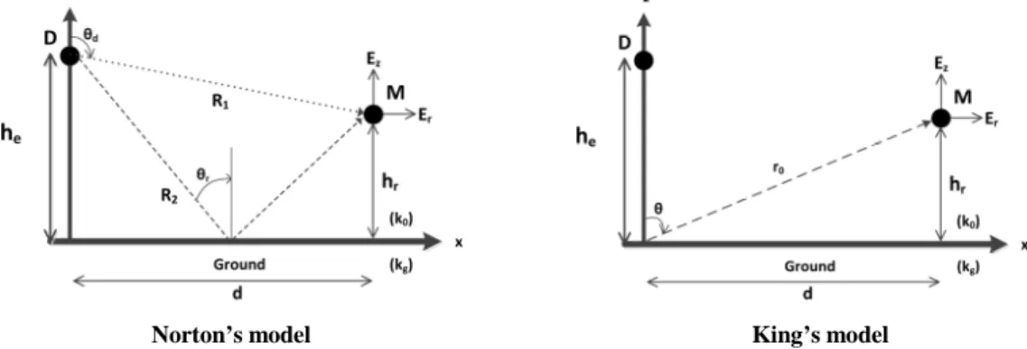
Fig. 2 describes the set of coordinates and the geometry parameters. Since the propagation characteristics are dependent on ground properties, we use the wave numbers k0 and kg, respectively in the air

and in the ground, where εrg and σg are respectively the relative

permittivity and the conductivity of the ground. These media are assumed to have the same permeability µ0 as that of free space.

( 1 )

( 2 )

( 3 )

Where εc is the complex refractive index of the ground.

A. Norton’s Model

The EM field radiated by an infinitesimal vertical electric dipole on the surface of the planar Earth was firstly analyzed by A. Sommerfeld [1]. Then, K.A. Norton simplified the calculation, the formalism and the interpretation [2], [3] by introducing the attenuation function. Norton’s formalism starts from the Hertz vector and Norton’s model is valid for any transmitter or receiver height (he or hr). The Hertz

vector expression Πz contains 3 terms: a direct wave, a reflected wave

and the surface wave. When the transmitter and the receiver are both located on the ground (he=hr=0 m), the direct and reflected

Norton’s model King’s model

Fig. 2. Set of coordinates and location of an infinitesimal vertical electric dipole (D) at a height he in the air (wave number k0) over the ground (wave

number kg).

components cancel each other out, and only the surface wave is propagated (third component in (4)).

( 4 )

Where Z0=120π is the free space impedance, Rv the Fresnel’s

reflection coefficient and F the attenuation function of the surface wave. Rv and F(p0) are defined with the following formula:

( 5 )

1-j ( 6 )

( 7 )

Where p0is the Sommerfeld numerical distance.

The parameters bg and pg are respectively a numerical distance and a

numerical velocity:

( 8 )

( 9 )

Where X is the loss tangent of the ground.

The relation between the magnetic field and the Hertz vector is:

( 10 )

Fig. 1. Path loss of the field radiated by a vertically polarized dipole at 10 MHz, 20 MHz, and 30 MHz over the sea water (SW) and over a dry ground (DG) versus distance [11].

Based on Norton’s theory, we have also investigated the ground type and the frequency dependence of surface waves. Fig. 1 depicts the path loss versus the distance for sea water (εrg=80 and σg=4 S/m), and

dry ground (εrg=8 and σg=0.04 S/m) [5], each at three frequencies

(10 MHz, 20 MHz, and 30 MHz). These results were calculated with L. Sevgi’s tool [11]. Whatever the frequency, we notice that the path losses over the sea are lower than over dry ground. As a result, at 30 MHz and for a distance of 50 km, the path loss over dry ground is 44 dB higher than over sea water. Likewise, over any grounds, the path losses of the surface wave become more important when the frequency increases. As a result, over a dry ground at 50 km, the path loss at 30 MHz is 30 dB higher than at 10 MHz.

B. King’s Model

R.W.P. King established the EM field expression generated by a vertical electric dipole located on or in the vicinity of Earth surface from Maxwell’s equations. According to [6], the transverse magnetic induction Bφ and associated electric field E are governed by the

formulas:

( 11 )

( 12 )

Where P0=k03d/2kg2 is the Sommerfeld numerical distance and F(P0)

is defined by the following formula:

( 14 )

Where, C2(P0)+iS2(P0) is the Fresnel integral and ω is the pulsation.

These formulas have been proposed with the following conditions issued from [4] and [6] respectively:

( 15 )

( 16 )

Where r0 is defined in Fig. 2.

In table I, we calculate |kg|/k0 versus ground characteristics and

frequencies. As a result, we notice that the condition |kg|≥3k0 is

verified in the HF band. But over a dry ground (poor conductivity and relative permittivity) in the UHF band, the initial condition (15) is not verified.

TABLE I. CALCULATION OF |KG|/K0VERSUS GROUND CHARACTERISTICS

(SEA WATER AND DRY GROUND) AND FREQUENCIES IN ORDER TO VERIFY THE CONDITION |KG|≥3K0 |kg|/k0 10 MHz 20 MHz 30 MHz Sea Water ε_{rg=80 ;} σ_g=4 S/m 85 27 10 Dry Ground ε_rg=8 ; σg=0.04 S/m 8 3.3 2.83

King’s theory describes physically surface-wave propagation behavior by defining characteristic distances: the critical distance dc,

and the intermediate distance di. The critical distance dc represents

the boundary of the planar Earth model and the intermediate distance di is a baseline which defines the modification of attenuation law of

the surface waves.

( 17 )

( 18 )

Where a is the Earth radius.

Table II contains several characteristic distances dc and di depending

on the environment and frequency. The critical distance dc varies

only with frequency, while the intermediate distance di varies both

with frequency and the ground characteristics.

There are two notions of horizon. First, the optical horizon is close to 37 km at sea level. Secondly, in the field of surface-wave propagation, the radio-electrical horizon dc is the electrical planar

Earth boundary. As well as the antenna dimensions, the electrical horizon depends on the wavelength. Fig. 3 sketches the propagation behavior and we can distinguish two main areas:

• Up to the intermediate distance di, the EM field decreases

as 1/d.

• Starting from di, the EM field decreases as 1/d².

Physically, the transition between the two areas is smooth. We call this transition area the “smoothly” attenuation. As a result, Fig. 3 sketches three cases of surface-wave propagation:

• At 10 MHz over sea water, the intermediate distance di is

close to dc. Consequently, the 1/d² field strength attenuation

is not achieved, but the “smoothly” attenuation is expected.

• At 20 MHz over sea water, the intermediate distance di is

equal to 17 km and the critical distance dc is equal to

58 km. Consequently, the three behaviors (1/d, smoothly, and 1/d² attenuation) are expected.

• At 30 MHz over sea water, the intermediate distance di is

equal to 8 km and the critical distance dc is equal to 50 km.

Consequently, the three behaviors (1/d, smoothly, and 1/d² attenuation) are expected.

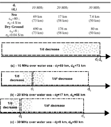
TABLE II. CHARACTERISTIC DISTANCES DI AND (DC) VERSUS SEVERAL

GROUND TYPES AND FREQUENCIES.

di (dc) 10 MHz 20 MHz 30 MHz Sea ε_rg=80 ; σ_g=4 S/m 69 km (73 km) 17 km (58 km) 7.6 km (50 km) Dry Ground ε_rg=8 ; σg=0.04 S/m 690 m (73 km) 176 m (58 km) 80 m (50 km)

Fig. 3. Behavior of the surface wave propagation along a path: according to the frequency and the ground type, the surface wave attenuation decreases as 1/d to reach smoothly 1/d². (a) – At 10 MHz over a sea water path, the surface field strength attenuation decreases as 1/d up to di=69 km ~ dc. (b) – At

20 MHz over a sea water path, the surface field strength attenuation decreases as 1/d over up to di=17 km, then decreases as 1/d² up to dc=58 km. (c) – At

30 MHz over a sea water path, the surface field strength attenuation decreases as 1/d over up to di=8 km, then decreases as 1/d² up to dc=50 km.

C. Millington’s Model

The Millington’s model is applied as soon as the environment contains several ground types along the propagation path. A simple case is sketched in Fig. 4 with two transitions through three media.

Fig. 4. Sketch of the Millington’s model: The transmitting antenna (Tx) is

located over the medium 1 while the receiver antenna (Rx) is located over the

medium 3. The medium 1 represents a segment range of length d1, the

medium 2 represents a segment range of length d2 and the medium 3

represents a segment of a variable length d.

According to Fig. 4, the semi empirical method can be explained with the following equations (19)-(21) coming from [11] and [14]: The total field ET along a multi-mixed propagation path at the

receiver is defined by:

( 19 )

Where ED and ER are respectively the fields along the direct and

reverse paths:

( 20 ) ( 21 )

Where E1, E2 and E3 are respectively the field over the medium 1, the

medium 2 and the medium 3.

The Millington’s method shows that the EM surface wave field strength is subject to the medium change. According to the modification of electrical ground characteristics, sea-ground or ground-sea, the EM field could respectively increase or decrease from each transition.

III. MEASUREMENT SETUP

1) Global description

This section presents the objectives of the measurements and describes the setup used to measure the attenuation of the electric field over the sea. The goals of our measurements are:

• To validate the 1/d and 1/d² attenuation of the surface wave propagation in the HF band calculated with the planar model.

• To validate Millington’s model.

In order to check the different attenuation behaviors over the sea, we have selected three frequencies (10 MHz, 20 MHz, and 30 MHz). The sea has been constantly calm (Sea State 0) all over the experimentation, so no sea roughness parameter has been considered in the theories.

The experimentation took place at the Mediterranean Sea in June 2013, at distances varying from the transmitting antennas. Fig. 5 depicts the environmental topography of the measurement area. The attenuation of the electric-field strength versus distance from the transmitting antennas was measured at 10, 20, and 30 MHz. Each measurement has been geo-localized and stored with an acquisition software developed by TDF. HF antennas installed on the coast (Tx)

have the capability to emit HF signal at each chosen frequency (10, 20, and 30 MHz) and the received signals are carried out with a loop antenna installed on a boat (Rx). The boat followed a southwestward

path across the Mediterranean Sea, steering a constant course. The three transmitting antennas operating respectively at 10 MHz, 20 MHz, and 30 MHz are located over salt ponds. A sand zone is located between the sea water and the transmitters. The relative permittivity εrg1 of the salt ponds is 80, and the conductivity σg1 is

8.8 S/m. For the sand transition, εrg2=8 and σg2=0.038 S/m. For the

sea water, εrg2=80 and σg2=5 S/m. The path over the salt ponds and

the sand is respectively 1 km and 6 km. These conductivities have been measured thanks to the following commercial devices:

• HANNA HI 993310 with HI 76305 probe for ground

• HANNA HI 9033 with HI 76302 probe for liquid

The measurements have been carried out in Continuous Waves (CW). No sky waves could be received, due to:

• A low Sunspot Number of 52.5 observed for June 2013

• A maximal path of 50 km

• A monopole shape radiation pattern for the transmitting antennas

This medium characteristic change allows observing the Millington’s effect.

• At 10 MHz, we measure the electric field strength from 9 km until 35 km. Consequently, the “smoothly” attenuation can be observed. At this frequency, the Millington’s effect is notable because of the sand transition.

• At 20 MHz, we measure the electric field strength from 6.5 km until 60 km. Consequently, the 1/d² attenuation can be observed. At this frequency, the Millington’s effect is more significant.

• At 30 MHz, we measure the electric field strength from 6.5 km until 50 km. Consequently, the 1/d² attenuation can be observed. At this frequency, the Millington’s effect increases.

Fig. 5. The measurement path over the sea by boat from the vicinity of the transmitter (Tx) until the receiver (Rx).

The measurement setup used 2 types of antennas (see Fig. 6 and Fig. 7). The transmitting antenna, a patented surface-wave antenna, called DAR antenna [19], has been manufactured by TDF (see Fig. 6). The antenna is manufactured with a steel galvanized wire with a diameter of 2.7 mm. Its dimensions have been adjusted according to the selected frequency. The horizontal radiation pattern is omnidirectional. Table III summarizes the horizontal length Lt, the

vertical height h, and the gap Ze of the DAR-antennas for each

frequency. The receiving antenna, a loop (see Fig. 7) installed on a boat, operates across a broad frequency band. The table IV presents the performance of the loop at 10, 20 and 30 MHz. The K-Factor is inversely proportional to the gain. So, the lower the K-factor, the higher the efficiency. The receiver antenna is installed 1 meter above the surface of the sea. A Rohde & Schwarz EB200 is used as the receiver.

Fig. 6. DAR-antenna design and tuning parameters: horizontal length (Lt) and vertical height (h).

Fig. 7. Receiver-antenna design: copper tube (16/14 mm) loop of 420 mm diameter

TABLE III. DIMENSIONS OF THE DAR-ANTENNAS.

10 MHz 20 MHz 30 MHz

Lt 6.37 m 2.52 m 1.83 m

h 1.8 m 1.8 m 1.5 m

Ze 0.5 m 0.5 m 0.5 m

TABLE IV. PERFORMANCES OF LOOP ANTENNA VERSUS FREQUENCY.

10 MHz 20 MHz 30 MHz

K – Factor

(dB/m) 42 41 43

The antenna gain has been measured in the relevant azimuth in order to calculate the electric field strength. The antenna gains at 10 MHz, 20 MHz, and 30 MHz are respectively 3.3 dBi, 5 dBi, and -1.3 dBi (see table V). The electric field strength E(d0) at 1 km is the reference

field used to normalize the theoretical models with the transmitting antenna characteristics. Thus, the reference field E(d0=1 km) at

10 MHz, 20 MHz, and 30 MHz is respectively 90.48 dBµV/m, 92.79 dBµV/m, and 88.24 dBµV/m.

TABLE V. MEASURED ANTENNA GAINS (DBI) AND THE ASSOCIATED ELECTRIC FIELD STRENGTH AT A DISTANCE D0=1 KM.

f (MHz) Antenna Gain _(dBi) Input power _{(dBm) (dBµV/m)} E(d0)

10 3.3 45 90.48

20 5 45 92.79

30 -1.3 47 88.24

IV. COMPARISON BETWEEN MEASUREMENTS AND THEORETICAL CALCULATION

1) The “smoothly” attenuation at 10 MHz

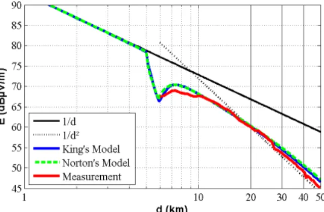
Fig. 8 presents the theoretical and the measured electric field along a 35 km mixed-path (salt ponds, sand, and sea water) at 10 MHz. 46 points per kilometers have been recorded. The theoretical models (King and Norton) and the measurement results are in good agreement besides a maximal deviation of 1.13 dB. The EM field attenuation slope is between the 1/d and 1/d² slopes. This behavior corresponds to the “smoothly” attenuation because the maximum measured distance (35 km) is lower than King’s intermediate distance di which is equal to 69 km. The decrease of electric field level is due

to the sand transition because the sand is a medium which is not suitable to the HF propagation.

2) The 1/d² attenuation and Millington’s effect at 20 MHz and

30 MHz

Fig. 9 presents the theoretical and the measured electric field along a 60 km mixed-path (salt ponds, sand, and sea water) at 20 MHz. 40 points per kilometers have been recorded. The theoretical models (King and Norton) and measurement results are in good agreement. The discrepancies between theories and measurements are less than 2 dB between 6 km and 10 km. From 30 km, the 1/d² attenuation is observed.

Fig. 8. Theoretical and measured electric field attenuation at 10 MHz over a mixed path: salt ponds, sand, and sea water. The theoretical results are calculated from Norton’s and King’s models. The red curve represents the measurements over the sea water.

Fig. 9. Theoretical and measured electric field attenuation at 20 MHz over a mixed path: salt ponds, sand, and sea water. The theoretical results are calculated from Norton’s and King’s models. The red curve represents the measurements over the sea water.

At 20 MHz, the effect of the sand transition is more significant than at 10 MHz. At the interface between the sand and the sea water (6 km), we notice small perturbations on the measured electrical fields. The sand transition includes a sand dune. This relief could induce diffraction and it could be the reason of this perturbation. The phenomenon has not been taken into account theoretically; a bigger change of the slope has been predicted.

Fig. 10 exhibits the theoretical and the measured electric fields along a 50 km mixed-path (salt ponds and sea water) at 30 MHz. 46 points per kilometers have been recorded. The theoretical models (King and Norton) and the measurement results are in good agreement. The maximal deviation between theories and measurements is close to 4 dB between 6 km and 10 km. Starting from 15 km, the 1/d² attenuation behavior is observed.

The perturbation, underlined at 20 MHz at the interface between the sand and the sea water, is amplified at 30 MHz because the relief is higher related to the wavelength.

Fig. 10. Theoretical and measured electric field attenuation at 30 MHz over a mixed path: salt ponds, sand, and sea water. The theoretical results are calculated from Norton’s and King’s models. The red curve represents the measurements over the sea water.

V. CONCLUSION

In this paper, the measurements of surface waves propagating along sea water path in the HF band are compared with theories. First of all,

we have described briefly the theoretical results proposed by Norton and King. Then, we have presented measurement results at 3 frequencies (10 MHz, 20 MHz and 30 MHz) and compared it to the theories including Millington’s modification in order to take into account the interface between the coast and water sea. At 10 MHz, the “smoothly” attenuation is shown and is very well correlated with the theory. The EM field decrease as 1/d² has been clearly observed at 20 MHz and 30 MHz.

A future work is scheduled to measure the electric field strength of the surface wave at larger distances in order to consider the roundness of Earth.

AKNOWLEDGEMENTS

The Authors thank warmly J. Y. Laurent from TDF for his technical support. They also thank TDF and Direction Générale de l’Armement for their funding.

REFERENCES

[1] A. Sommerfeld, “Propagation of waves in wireless telegraphy,” Ann. Phys., vol 28, pp. 665-736, 1909

[2] K.A. Norton, “The propagation of radio waves over the surface of the earth and upper atmosphere - PART 1,” Proceeding of the institute of radio engineers, 1936

[3] K.A. Norton, “The propagation of radio waves over the surface of the earth and upper atmosphere - PART 2,” Proceeding of the institute of radio engineers, 1937

[4] R. W. P. King, “On the radiation efficiency and the electromagnetic field of a vertical electric dipole in the air above a dielectric or conducting half-space,” in Progress in Electromagnetic Research, J. A. Kong, Ed. New York: Elsevier, vol. 4, ch. 1, 1990

[5] R. W. P. King, S. S. Sandler, “The electromagnetic field of a vertical electric dipole over the Earth or sea,” Antennas and Propagation, IEEE Transactions on , vol. 42, no. 3, pp. 382-389, Mar. 1994

[6] R. W. P. King, C. W. Harrison, “Electromagnetic ground-wave field of vertical antennas for communication at 1 to 30 MHz,” Electromagnetic Compatibility, IEEE Transactions on , vol. 40, no. 4, pp. 337-342, Nov. 1998

[7] J. R. Wait, Electromagnetic Waves in Stratified Media, New York, Pergamon Press, first edition 1 962; second enlarged edition 1970; first edition reprinted by IEEE Press 1996

[8] J. R. Wait, “The ancient and modern history of EM ground-wave propagation,” Antennas and Propagation Magazine, IEEE , vol. 40, no. 5, pp. 7-24, Oct. 1998

[9] G. Millington, “Ground-wave propagation over an inhomogeneous smooth earth,” Proceedings of the IEE - Part III: Radio and Communication Engineering , vol. 96, no. 39, pp. 53-64, Jan. 1949 [10] G. Millington, G.A. Isted, “Ground-wave propagation over an

inhomogeneous smooth earth. Part 2: Experimental evidence and practical implications,” Electrical Engineers, Journal of the Institution of , vol. 1950, no. 7, pp. 190-191, July 1950

[11] L. Sevgi, “A mixed-path groundwave field-strength prediction virtual tool for digital radio broadcast systems in medium and short wave bands,” Antennas and Propagation Magazine, IEEE , vol. 48, no. 4, pp. 19-27, 4, Aug. 2006

[12] L. Sevgi, F. Akleman; L. B. Felsen, “Groundwave propagation modeling: problem-matched analytical formulations and direct numerical techniques,” Antennas and Propagation Magazine, IEEE , vol. 44, no. 1, pp. 55-75, Feb. 2002

[13] L. Sevgi, “Groundwave Modeling and Simulation Strategies and Path Loss Prediction Virtual Tools,” Antennas and Propagation, IEEE Transactions on , vol. 55, no. 6, pp. 1591-1598, June 2007

[14] L. Boithias, "Propagation des ondes radioélectriques dans l’environnement terrestre", Dunod, 1983

[15] IUT-R, “Ground-wave propagation curves for frequencies between 10 kHz and 30 MHz,” http://www.itu.int/pub/R-REC/fr

[16] IUT-R,“Calculation of free space attenuation,” http://www.itu.int/pub/R-REC/fr

[17] S. Rotheram, “Ground-wave propagation. Part 1: Theory for short distances,” Communications, Radar and Signal Processing, IEE Proceedings F , vol. 128, no. 5, pp. 275,284, Oct. 1981

[18] http://www.ips.gov.au/Products_and_Services/1/4

[19] S. Palud, P. Piole, P.Y. Jezequel, J.Y. Laurent, L. Prioul, “ Large-area broadband surface-wave antenna,” Patent WO/2012/045847