Optimisation de tubes à vortex à air par des modèles analytiques et numériques

Faculté de génie

Département de génie mécanique

OPTIMISATION DE TUBES À VORTEX À

AIR PAR DES MODÈLES ANALYTIQUES

ET NUMÉRIQUES

Thèse de doctorat

Spécialité : génie mécanique

Junior LAGRANDEUR

Sherbrooke (Québec) Canada

Sébastien PONCET

Mikhail SORIN

Martin BROUILLETTE

Hakim NESREDDINE

Anthony STRAATMAN

Bo ZHANG

Les tubes à vortex permettent de séparer un gaz comprimé entrant à une température

intermé-diaire en un écoulement chaud et un écoulement froid. Toutefois, leur faible efficacité

exergé-tique limite leurs applications. Il est difficile d’optimiser un tube à vortex pour chaque

applica-tion étant donné que le mécanisme de transfert de chaleur reste encore mal compris.

Dans cette thèse, plusieurs techniques sont combinées afin d’éclaircir le mécanisme de fonction-nement des tubes à vortex à contre-courant et d’en prédire les performances. Tout d’abord, une revue de la littérature des modèles analytiques prédictifs permet d’analyser les modes de fonc-tionnement proposés des tubes à vortex sous l’angle de leur capacité à prédire les performances. Aucun des modèles ne prédit adéquatement les performances des tubes, mais cette revue de la littérature a permis d’éliminer déjà quelques options, dont le modèle de l’échangeur de chaleur. Plusieurs des modèles analytiques présentés utilisent le ratio de pression entre l’entrée et la sortie pour calculer les performances du tube. Ce paramètre permet de calculer les propriétés à l’entrée dans un nouveau modèle analytique. Ce modèle calcule la vitesse d’entrée de façon à obtenir un gradient de pression interne correspondant à un vortex forcé. Il utilise aussi un profil de température statique isotherme sur le plan d’entrée pour calculer les températures de sortie. Celui-ci se compare avantageusement avec des résultats expérimentaux issus de la littérature. Ensuite, deux réseaux de neurones artificiels entrainés à partir de mesures provenant de 11

sources différentes prédisent la température de sortie froide et le débit massique à partir d’un

nombre réduit de paramètres d’entrée. Les paramètres retenus sont ceux ayant le plus d’influence sur la performance des tubes. Seule la longueur n’est pas utilisée dans le modèle analytique. Ces deux méthodes ont permis d’optimiser la géométrie du tube à vortex. La configuration op-timale identifiée à l’aide des réseaux de neurones correspond à une condition avec peu de

résul-tats expérimentaux. Pour le modèle analytique, celui-ci a optimisé l’efficacité exergétique d’un

tube à vortex et de combinaisons de tubes à vortex en cascade. Comme ce modèle se base sur une meilleure connaissance du mode de fonctionnement, il a également identifié les principales sources de destruction d’exergie à l’intérieur et à l’extérieur du tube.

Finalement, les modélisations numériques de l’écoulement viennent complèter le modèle ana-lytique. Toutefois, certaines hypothèses sous-jacentes sont inadéquates. Le gradient de pression crée l’échange de chaleur. La conductivité thermique turbulente n’en tient pas compte. Le

mo-dèle k−ω SST avec un solveur basé sur la densité et un terme source additionnel dans l’équation

d’énergie permet de prédire adéquatement la température de sortie froide et la pression de sortie

chaude lorsque la fraction massique froide (µc) est élevée. Lorsque µcest plus faible, les modèles

de turbulence analysés ne prédisent pas correctement l’éclatement tourbillonnaire dans le tube froid, expliquant leur mauvaise performance sous ces conditions. Des pistes d’amélioration sont proposées pour améliorer le résultat des simulations.

Mots-clés : tube à vortex, modèle thermodynamique, réseaux de neurones artificiels, exergie, modélisations numériques, éclatement tourbillonaire, couche limite de Bödewadt

OPTIMIZATION OF AIR VORTEX TUBES BY ANALYTICAL AND NUMERICAL MODELS

Vortex tubes separate a compressed gas at an intermediate temperature into a cold stream and

a hot stream. However, their low exergetic efficiency limits their applications. Optimizing

vortex tubes for a specific application is difficult because the heat transfer mechanism is not

well understood.

This thesis explains the working mechanism of vortex tubes and predicts their performance using

different techniques. To begin, this thesis presents a review of predictive models for vortex

tubes. This review analyzes theory about the vortex tube working mechanism based on their ability to predict their performance. None of the reviewed models is able to predict vortex tubes’ performance. Some model may be discarded, including the heat exchanger analogy. Many of the reviewed models use the pressure ratio between the inlet and the cold outlet to predict vortex tubes’ performance. This ratio is used to calculate the inlet velocity to match the pressure gradient generated by a forced vortex in a new analytical model. In addition, this model assumes an isothermal static temperature profile on the inlet plane to calculate the cold outlet temperature. This new model predicts adequately the cold outlet temperature of two vortex tubes studied experimentally in the literature.

Thirdly, two artificial neural networks (ANN) are trained from 600 measurements from 11 dif-ferent sources available in the literature. These two ANN models predict accurately the cold outlet temperature and the mass flow rate from a limited number of parameters. From these, only the vortex tube length is not used in the analytical model.

One uses these two methods to optimize the geometry of the vortex tube. The optimal configu-ration identified by the ANN models corresponds to a condition with few experimental results.

The analytical model optimizes the exergetic efficiency of both a single vortex tube and a

cas-cade of vortex tubes. In addition, because this model provides a deeper understanding of the heat exchange mechanism, the model identifies the main sources of exergy destruction inside and outside the vortex tube.

Finally, results from numerical simulations complete the outcomes of the analytical model. However, some underlying assumptions are inappropriate. The pressure gradient generates the

heat exchange. The turbulent thermal conductivity assumption does not include this effect. The

k− ω SST model coupled with the density-based solver and an additional source term in the

en-ergy equation predict the right cold outlet temperature for high cold mass fractions (µc). When

µc is lower, the investigated turbulence models do not predict correctly the vortex breakdown

in the cold tube. This may explain the poor performance of these models under this condition. Some improvements to standard turbulence models are finally proposed.

Keywords: vortex tube, thermodynamic modeling, artificial neural networks, exergy, turbulence modeling, vortex breakdown, Bödewadt boundary layer

Je tiens tout d’abord à remercier mes directeurs de thèse, les professeurs Sébastien Poncet et Mikhail Sorin. Faire un doctorat sans avoir fait de recherche depuis huit ans et avec cinq enfants était un projet fou, mais vous y avez cru et m’avez aidé à rendre le tout possible. Merci, Sé-bastien, pour ta grande disponibilité et ton soutien constant. Merci, Mikhail, pour les pistes de recherche inspirantes que tu m’as proposées et qui m’ont permis de développer et d’exploiter le nouveau modèle analytique présenté dans cette thèse.

Je tiens particulièrement à remercier mon collègue Sergio Croquer. Tu m’as bien enseigné la CFD. Ta disponibilité et ta patience m’ont été d’un grand secours pour réaliser cette thèse. Je remercie également mes collègues du LMFTEUS, particulièrement Alla Eddine, Yu, Hazhir, Mohamad et Abbas. Nos discussions et notre camaraderie m’ont souvent permis d’égayer ma journée et d’éclairer mon esprit.

Je remercie également les évaluateurs, Martin Brouillette, Antony Straatman, Bo Zhang et Ha-kim Nesreddine, d’avoir accepté de réviser cette thèse.

Je remercie aussi Carl Binette d’Aéronergie pour avoir cru en moi. Ce projet était risqué, mais

le financement offert pendant 18 mois par le biais du programme Mitacs Accélération a rendu le

doctorat possible. J’espère que nous pourrons collaborer sur d’autres projets à l’avenir.

Je tiens aussi à remercier le Conseil national de recherche du Canada, le Fonds de recherche du Québec - Nature et technologie, Ingénieurs Canada, le centre CREEPIUS et la chaire CRSNG (Hydro-Québec, Ressources Naturelles Canada et Emerson Canada) pour m’avoir octroyé des bourses pour mon doctorat.

Je tiens finalement à remercier toute ma famille, et plus particulièrement mon épouse Caroline et mes enfants Ali, Lily-Rose, Léa, Édouard et Henri. Vous m’avez soutenu et vous avez ac-cepté de faire des sacrifices pour me permettre de réaliser ce rêve. Sans votre appui et votre compréhension, cette thèse n’aurait jamais pu voir le jour.

1 Introduction 1

1.1 Mise en contexte et problématique . . . 1

1.2 Question de recherche . . . 2

1.3 Objectifs du projet de recherche . . . 3

1.4 Contributions originales . . . 3

1.5 Plan du document . . . 5

1.6 Context and Problematic . . . 7

1.7 Research’s Question . . . 8

1.8 Project Objectives . . . 8

1.9 Original Contributions . . . 9

1.10 Document Organization . . . 11

2 Revue des modèles prédictifs pour la conception de tubes à vortex à contre-courant utilisant un gaz parfait 13 2.1 Introduction . . . 16

2.2 Scope of the Present Review . . . 17

2.3 Description of Predictive Models . . . 18

2.3.1 Empirical Methods for Engineering Purpose . . . 18

2.3.2 First and Second Thermodynamic Laws in Vortex Tubes . . . 20

2.3.3 Vortex Tube as an Heat Exchanger . . . 24

2.3.4 Model Based on a Pressure Gradient . . . 27

2.3.5 Gas Dynamics Model . . . 33

2.3.6 Large Scale Unsteadiness . . . 41

2.4 Discussion . . . 45

2.5 Conclusion . . . 49

3 Modélisation à l’aide d’un modèle thermodynamique et de réseaux de neurones artificiels 51 3.1 Introduction . . . 54

3.2 Artificial neural networks . . . 57

3.2.1 Basic principles . . . 57

3.2.2 Proposed ANN models . . . 58

3.2.3 Features selection . . . 59

3.2.4 Parametric optimizations using the ANNs . . . 62

3.3 Thermodynamic modeling . . . 72

3.3.1 Main hypotheses . . . 72

3.3.2 Development of the thermodynamic model . . . 74

3.3.3 Influence of the pressure losses . . . 75

3.3.4 Effect of the Bödewadt boundary layer flow . . . 78

3.4 Comparing ANN and thermodynamic models outputs with experimental data . . 79

3.5 Discussion . . . 81

3.5.1 Artificial neural networks . . . 81

3.5.2 Thermodynamic model . . . 82

3.6 Conclusion . . . 83

4 Analyse exergétique de l’écoulement et optimisation exergétique de tubes à vortex utilisant de l’air 87 4.1 Introduction . . . 90

4.2 Efficiency Metrics . . . 94

4.3 Exergetic Efficiency for a Single Vortex Tube . . . 98

4.3.1 Outlet Temperature Calculation . . . 98

4.3.2 Exergy Generation and Destruction in Vortex Tubes . . . 101

4.3.3 Exergy Transformation Inside the Vortex Tube . . . 108

4.4 Parametric Optimization of the Vortex Tube . . . 110

4.4.1 Cold Outlet to the Atmosphere . . . 112

4.4.2 Swirl Decay Inside the Cold Pipe . . . 114

4.5 Optimum System Configuration . . . 115

4.5.1 Single Vortex Tube . . . 116

4.5.2 Cascade configuration starting with the optimal vortex tube . . . 118

4.5.3 Cascade configuration ending with the optimal vortex tube in the cold cascade . . . 118

4.5.4 Cascade configuration with identical pressure ratio . . . 118

4.5.5 Cold cascade with an ejector . . . 119

4.6 Discussion . . . 121

4.7 Conclusion . . . 122

5 Modélisation numérique d’un tube à vortex de Ranque-Hilsch en se référant à la fraction massique froide 125 5.1 Introduction . . . 128

5.2 Numerical Method . . . 133

5.2.1 Computational Domain . . . 133

5.2.2 Governing Equations and Numerical Algorithms . . . 134

5.2.3 Turbulence Models . . . 135

5.2.4 Boundary Conditions . . . 136

5.2.5 Mesh Grids . . . 137

5.2.6 Fractional Factorial Design . . . 138

5.3 Results and Discussion . . . 139

5.3.1 Fractional Factorial Design . . . 139

5.3.2 Prediction of the Cold Mass Fraction and Cold Outlet Temperature at an Intermediate Pressure . . . 146

5.3.3 Effect of the Additional Source Term in the Energy Equation . . . 152

5.3.4 Interior Velocity Profiles . . . 153

5.4 Conclusion . . . 156

6 CONCLUSION 161 6.1 Contributions originales . . . 161

6.1.1 Modèle analytique . . . 161

6.1.2 Réseaux de neurones artificiels . . . 163

6.1.3 Modélisations numériques . . . 164 6.2 Perspectives . . . 165 6.2.1 Applications . . . 165 6.2.2 Modèle analytique . . . 169 6.2.3 Modélisations numériques . . . 170 7 ENGLISH CONCLUSION 173 7.1 Original Contribution . . . 173 7.1.1 Analytical Model . . . 173

7.1.2 Artificial Neural Networks . . . 175

7.1.3 Computational Fluid Dynamic . . . 176

7.2 Research perspectives . . . 177

7.2.1 Applications . . . 177

7.2.2 Analytical Model . . . 180

7.2.3 Computational Fluid Dynamics . . . 181

A Résultats additionnels des simulations numériques : Plans d’expérience 185

B Résultats additionnels des simulations numériques : Terme source additionnel 227

2.1 Schematic drawing of a counterflow vortex tube. . . 16

2.2 Comparison of actual COP from 12 different authors and isentropic ideal COP. . 21

2.3 Representative behaviour of temperature separation and entropy generation in a

vortex tube. . . 23

2.4 Flow pattern for the heat exchange process across an imaginary tube. . . 25

2.5 Heat transfer process from particles embedded in turbulent eddies. . . 29

2.6 Schematic view showing the heat exchange by turbulent eddies in a vortex tube. 30

2.7 Contour plots of T/pγ−1γ _{from a CFD simulation using the standard k}− ϵ

turbu-lence model. . . 31

2.8 Schematic view showing the heat pump model based on the secondary circulation. 33

2.9 Hypothetical flow patterns (top) from experimental measurements of the swirl,

axial and radial velocity components. . . 35

2.10 Contour plots showing the temperature (top), the shear stress (middle) and the

geometry of the vortex folding inward (bottom). . . 36

2.11 The elementary propulsion system of Polihronov and Straatman. . . 37

2.12 Schematic of the system model by Tuytyuma and Allahverdyan and Fauve. . . . 38

2.13 The dimensionless profiles of the tangential velocity for different radial

Rey-nolds numbers for two different radius ratios. . . 39

2.14 Representative nearly axisymmetric vortex breakdown in water. . . 42

2.15 Isosurface of the instantaneous axial velocity uz = 0 showing a periodic

revolu-tion of the vortex core. . . 43

2.16 Instantaneous streamlines of a vortex tube in a LES simulation. . . 44

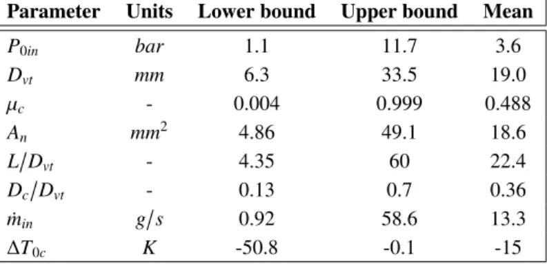
3.1 Schematic flow structure inside a counterflow vortex tube. . . 55

3.2 Mean square errors of the ANN models as a function of the number of iterations. 61

3.3 Linear regression coefficients obtained by the ANN model for the estimation of

∆T0c. . . 63

3.4 Linear regression coefficients obtained by the ANN model for the estimation of

˙

min. . . 64

3.5 Estimation of ˙min as a function of An and L/Dvt for two different values of P0in

and Dvt using the ANN. . . 65

3.6 Estimation of the cold outlet temperature drop as a function of µc and L/Dvtfor

two different values of P0in and three different ratios Dc/Dvt. Results obtained

by the ANN model. . . 67

3.7 Prediction of COP as a function of µcand L/Dvtfor two different values of P0in

and the optimum value of Dc/Dvt. Results obtained by the ANN model. . . 68

3.8 Estimation of the cooling power as a function of µc and L/Dvtfor two values of

P0in and three different ratios Dc/Dvt. Results obtained by the ANN model. . . . 69

3.9 Scatter plot matrix of the most significant input data for the estimation of ˙min. . . 70

3.10 Scatter plot matrix of the most significant input data for the estimation of∆Tc. . 71

3.11 Distributions of the cold outlet pressure as a function of the cold mass fraction

for different inlet pressures and two references. . . 73

3.12 Schematic of the flow structure and of the main hypotheses used to model the

vortex tube. . . 74

3.13 Cold outlet temperature as a function of the cold mass fraction. Comparison between the base thermodynamic model with the experimental data from Camiré

for P0in =3.08 bar. . . 76

3.14 Cold outlet temperature computed by the model of Liew et al., the present ther-modynamic model and the ANN model. Comparison with the experimental data

from Camiré for four different inlet pressures. . . 80

3.15 Cold outlet temperature computed by the model of Liew et al., the present ther-modynamic model and the ANN model. Comparison with the experimental data

from Skye et al.for P0in=5.7 bar. . . 80

4.1 The optimal flow structure inside a counterflow vortex tube. . . 93

4.2 Schematic of the air cycle used to define the COP. . . 96

4.3 Cold outlet temperature as a function of the inlet pressure and cold mass fraction.

Comparison between the original model, the corrected temperature prediction

and the experimental data from Camiré. . . 99

4.4 Cooling power and heating power calculated from the experimental data of Camiré.100

4.5 T0h as a function of the inlet pressure and cold mass fraction . Comparison

bet-ween the corrected model’s temperature prediction , the experimental data from

Camiré and T0h computed from the experimental cold outlet temperature using

the conservation of energy. . . 102

4.6 Exergy efficiency of the vortex tube when ∆e is divided by the total available

mechanical exergy. . . 103

4.7 Mechanical exergy consumed in the vortex tube process. . . 106

4.8 Exergetic efficiency with only the exergy consumed in the vortex tube as the

denominator. . . 107

4.9 Illustration of the various steps in the energy separation process from the

ther-modynamic model . . . 109 4.10 Grassmann diagram showing the exergy consumed and transiting at each step of

the energy separation process. . . 109

4.11 The normalized pressure drop across the vortex tube as a function of ˙mh after

the experimental data of Camiré. . . 112 4.12 Flowchart of the calculation process used to optimize the vortex tube. . . 113 4.13 Schematic of the cold cascade using an ejector. . . 120

5.1 Total temperature contours (in K) in a vortex tube with the main flow features

and the vortex tube dimensions. Results obtained by CFD using mesh 2, the

k− ω SST model, density-based implicit solver and variable physical properties

for condition 7 in Table 5.5. . . 129

5.3 Influence of the turbulence model and of the solver type on the prediction error

for the cold mass fraction (∆µc) with mean values for P0in and nominal µc.▲:

density-based solver ;∎: pressure-based solver . . . 142

5.4 Mach number contours near the inlet for case 16 of Table 5.6. . . 142

5.5 Streamlines at the cold outlet of the vortex tube for simulation 2 of Table 5.6.

Streamlines are colored by the velocity magnitude in m⋅s−1. This figure clearly

shows a recirculation zone along the axis. . . 143

5.6 Influence of P0in and µc on Ls with variable properties, density-based solver,

mesh 2 and k−ω SST turbulence model. ∎ : nominal µc=0.4;▲: nominal µc=0.7;144

5.7 Ratio of the absolute tangential velocity to the absolute axial velocity in the cold

tube and near the inlet. Figures obtained from cases 2 and 10 from Table 5.6

(P0in=1.7 bar, nominal µc=0.4, k− ω SST, fixed properties). . . 145

5.8 Comparison in terms of the cold outlet temperature between the experimental

values of Camiré [32] and the present numerical predictions when using both ex-perimental outlet pressure values at the boundaries. All simulations are

steady-state and use the density-based solver except where specified otherwise. ▲ :

reference ;∎ : k− ω SST, mesh 1;● : k− ω SST, mesh 2;⧫ : k− ϵ mesh 1; ▲:

k− ω SST, mesh 1, unsteady; + : k − ω SST, mesh 1, pressure-based solver; X :

k− ω SST, mesh 2, Skh; – : RSM, mesh 1, transient. The black line represent all

experimental results at this condition. . . 147

5.9 Comparison in terms of the cold outlet temperature between the experimental

values of Camiré [32] and the present numerical predictions when using the experimental cold outlet pressure and changing the hot outlet pressure to get the

experimental µcvalue. All simulations are steady-state and use the density-based

solver except where specified otherwise.▲: reference ;∎: k−ω SST, mesh 1;●:

k−ω SST, mesh 2;⧫: k−ϵ mesh 1; + : k−ω SST, mesh 1, pressure-based solver;

X : k− ω SST, mesh 2, Skh;◻ : analytical model of Lagrandeur et al. [102]. The

black line represent all experimental results at this condition. . . 147

5.10 Turbulent viscosity ratio for three turbulence models at P0in=2.4 bar and µc=0.6.

Results obtained with variable properties. The hot outlet pressure is adjusted to

obtain the experimental µcfor for k− ω SST and k − ϵ, but not for the RSM. . . . 148

5.11 Static temperature (K) for P0in=2.4 bar and µc=0.6. Results obtained with

va-riable properties. The hot outlet pressure is adjusted to obtain the experimental

µc for k− ω SST and k − ϵ, but not for the RSM. . . 149

5.12 Ratio between the tangential and axial velocity components for P0in=2.4 bar

and µc=0.6. Results obtained with variable properties. The hot outlet pressure is

adjusted to obtain the experimental µcfor k−ω SST and k−ϵ, but not for the RSM.151

5.13 Difference between the experimental hot outlet pressure and the value used in

the numerical model (DPh) to get the same µc result. All simulations are

steady-state and use the density-based solver except where specified otherwise. ▲ :

reference ;∎ : k− ω SST, mesh 1;● : k− ω SST, mesh 2;⧫ : k− ϵ mesh 1; + :

k− ω SST, mesh 1, pressure-based solver; X : k − ω SST, mesh 2, Skh. . . 152

5.14 Contours of (a) the radial velocity profile and (b) the density gradient near the

inlet section. Steady-state results obtained for P0in=2.4 bar, µc=0.6, mesh 2, k−

5.15 Tangential velocity profile at the (a) inlet, (b) L/2 and axial velocity profile at

(c) L/2. Results obtained using the k− ω SST model (△) on mesh 2 and the

RSM k− ω BSL model on mesh 1 (◯) and from experimental measurements of

Camiré [32] (●). Both profiles are from unsteady simulations using the

density-based solver at conditions of case 7, Table 5.5. . . 155

6.1 Schéma préliminaire intégrant un tube à vortex en amont d’une pile à combus-tible PEM embarquée dans un véhicule. . . 167

7.1 Preliminary diagram integrating a vortex tube upstream of a PEM fuel cell on board a vehicle. . . 178

A.1 Static temperature for P0in=1.7 and nominal µc=0.4. . . 187

A.2 Static temperature for P0in=1.7 and nominal µc=0.7. . . 188

A.3 Static temperature for P0in=3.08 and nominal µc=0.4. . . 189

A.4 Static temperature for P0in=3.08 and nominal µc=0.7. . . 190

A.5 Total temperature for P0in=1.7 and nominal µc=0.4. . . 191

A.6 Total temperature for P0in=1.7 and nominal µc=0.7. . . 192

A.7 Total temperature for P0in=3.08 and nominal µc=0.4. . . 193

A.8 Total temperature for P0in=3.08 and nominal µc=0.7. . . 194

A.9 Axial velocity for P0in=1.7 and nominal µc=0.4. . . 195

A.10 Axial velocity for P0in=1.7 and nominal µc=0.7. . . 196

A.11 Axial velocity for P0in=3.08 and nominal µc=0.4. . . 197

A.12 Axial velocity for P0in=3.08 and nominal µc=0.7. . . 198

A.13 Radial velocity for P0in=1.7 and nominal µc=0.4. . . 199

A.14 Radial velocity for P0in=1.7 and nominal µc=0.7. . . 200

A.15 Radial velocity for P0in=3.08 and nominal µc=0.4. . . 201

A.16 Radial velocity for P0in=3.08 and nominal µc=0.7. . . 202

A.17 Tangential velocity for P0in=1.7 and nominal µc=0.4. . . 203

A.18 Tangential velocity for P0in=1.7 and nominal µc=0.7. . . 204

A.19 Tangential velocity for P0in=3.08 and nominal µc=0.4. . . 205

A.20 Tangential velocity for P0in=3.08 and nominal µc=0.7. . . 206

A.21 Ratio of the tangential velocity and the axial velocity for P0in=1.7 and nominal µc=0.4. . . 207

A.22 Ratio of the tangential velocity and the axial velocity for P0in=1.7 and nominal µc=0.7. . . 208

A.23 Ratio of the tangential velocity and the axial velocity for P0in=3.08 and nominal µc=0.4. . . 209

A.24 Ratio of the tangential velocity and the axial velocity for P0in=3.08 and nominal µc=0.7. . . 210

A.25 Static pressure for P0in=1.7 and nominal µc=0.4. . . 211

A.26 Static pressure for P0in=1.7 and nominal µc=0.7. . . 212

A.27 Static pressure for P0in=3.08 and nominal µc=0.4. . . 213

A.28 Static pressure for P0in=3.08 and nominal µc=0.7. . . 214

A.29 Static density for P0in=1.7 and nominal µc=0.4. . . 215

A.31 Static density P0in=3.08 and nominal µc=0.4. . . 217

A.32 Static density for P0in=3.08 and nominal µc=0.7. . . 218

A.33 Turbulence kinetic energy for P0in=1.7 and nominal µc=0.4. . . 219

A.34 Turbulence kinetic energy for P0in=1.7 and nominal µc=0.7. . . 220

A.35 Turbulence kinetic energy P0in=3.08 and nominal µc=0.4. . . 221

A.36 Turbulence kinetic energy for P0in=3.08 and nominal µc=0.7. . . 222

A.37 Turbulent viscosity for P0in=1.7 and nominal µc=0.4. . . 223

A.38 Turbulent viscosity for P0in=1.7 and nominal µc=0.7. . . 224

A.39 Turbulent viscosity P0in=3.08 and nominal µc=0.4. . . 225

A.40 Turbulent viscosity for P0in=3.08 and nominal µc=0.7. . . 226

B.1 Static temperature using the additional energy source . . . 229

B.2 Total temperature using the additional energy source . . . 230

B.3 Axial velocity using the additional energy source . . . 231

B.4 Radial velocity using the additional energy source . . . 232

B.5 Tangential velocity using the additional energy source . . . 233

B.6 Ratio of the tangential velocity and the axial velocity using the additional energy source . . . 234

B.7 Static pressure using the additional energy source . . . 235

B.8 Static pressure gradient magnitude using the additional energy source . . . 236

B.9 Static density using the additional energy source . . . 237

B.10 Turbulence kinetic energy using the additional energy source . . . 238

2.1 Summary of model for vortex tubes’ performance prediction . . . 46

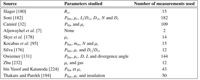
3.1 Experimental studies of counterflow vortex tubes working with air used to train,

validate and test the two ANN models. . . 60

3.2 Range of inputs and outputs for the data presented in Table 3.1 and the most

relevant parameters. . . 61

3.3 Optimum values of Dc/Dvt, L/Dvtand µc found in the literature. . . 66

3.4 Influence of the proposed improvements on the prediction of T0cfor P0in = 3.08

bars and µc= 0.6965. Results obtained by the thermodynamic model. . . 75

4.1 Specific exergy at various steps inside the vortex tube. Results obtained by the

thermodynamic model. . . 108

4.2 Optimum working conditions according to different performance criteria when

the vortex tube discharges directly to the atmosphere. . . 113

4.3 Optimum working conditions of the vortex tube at ¯Pc= 1 bar. . . 114

4.4 Optimum working conditions of the vortex tube at ¯Pc= 3 bars. . . 115

4.5 Optimum working conditions of the vortex tube at ¯Pc = 1 bar, but with T0in= 265

K (L) or T0in= 380 K (H) and Tre f = 295 K. . . 116

4.6 Vortex tubes combinations when the efficiency of the first tube is maximized. . . 117

4.7 Vortex tubes combinations when the efficiency of the last tube is maximized. . . 117

4.8 Vortex tubes cascades with identical pressure ratio for the two vortex tubes of

the cold cascade . . . 117

4.9 Optimization of the first vortex tube according to ηcfor various µc and the

asso-ciated ejector’s outlet conditions. T0p= 295 K for all cases. . . 120

4.10 Characteristic of the last vortex tube in the ejector-based configuration. . . 121

5.1 Former numerical studies on the predictions of air vortex tubes . . . 130

5.2 Main dimensions of the vortex tube. . . 133

5.3 Mesh independence study for case 4 of Table 5.5. . . 138

5.4 Factors investigated using the fractional factorial design method and their levels 138

5.5 Input parameters used for the different simulations. Experimental data extracted

from Camiré [32]. . . 139

5.6 Summary of the numerical results following the fractional factorial design

sche-dule. Svtand Sctare swirl numbers calculated using Eq. 5.7 at one diameter from

the inlet in the vortex tube and in the cold tube. Ls is the distance between the

stagnation point and the inlet. The last two columns show the difference between

the experimental and the calculated values for the cold outlet temperature (∆T0c

and the cold mass fraction (∆µc). . . 141

Symb. Définition anglaise Définition française Unités

A input weight on the hidden

layer in ANN or scaling factor or surface area

poids des neurones d’entrée sur ceux dans la couche caché ou facteur de mise à l’échelle ou surface

-, -, m2

b nozzle width largeur des buses d’entrée m

B hidden layer weight on the

output in ANN

poids des neurones de la couche cachée sur la sortie

-C input weight on the output

in ANN

poids des neurones d’entrée sur la sortie

-Cp specific heat at constant

pressure

chaleur spécifique à pression constante J⋅ kg−1⋅ K−1

Cv specific heat at constant

volume

chaleur spécifique à volume constant J⋅kg−1⋅K−1

Cµ empirical constant of the

k− ϵ model

constante empirique du modèle k− ϵ

-D diameter diamètre mm, m

Dµc error on µc prediction erreur sur la prédiction de µc

-e specific exergy exergie spécifique kJ⋅kg−1

E total exergy exergie totale W

˙

Eloss rate of exergy destruction taux de destruction d’exergie W

g gravitational acceleration accélération gravitationnelle m⋅s−2

h nozzle height or specific

enthalpy

hauteur des buses d’entrée ou enthalpie spécifique

m, J⋅kg−1

k turbulence kinetic energy énergie cinétique de la turbulence m2⋅s−2

kl laminar kinetic energy énergie cinétique laminaire m2⋅s−2

L vortex tube length (or

following the indices)

longueur du tube à vortex (ou selon l’indice)

mm, m

Ma Mach number nombre de Mach

-˙

m mass flow rate débit massique g⋅s−1

N number of nozzles nombre de buses d’entrée

-P pressure pression Pa

Prt turbulent Prandlt number nombre de Prandlt turbulent

-q specific cooling or heating

energy

énergie spécifique de chauffage ou de

refroidissement

kJ.kg−1

Q cooling or heating power puissance de chauffage ou de

refroidissement

W

Symb. Définition anglaise Définition française Unités

r radius rayon mm, m

Ra average surface roughness rugosité moyenne de surface µm

R, Rg specific perfect gas constant constante spécifique des gaz

parfaits

J⋅kg−1⋅K−1

Re Reynolds number nombre de Reynolds

-s specific entropy entropie spécifique J⋅kg−1⋅K−1

S swirl number nombre de swirl

-Skh additional source term in the

energy equation from Khait et

al.[88]

terme source additionnel de Khait

et coll.[88] dans l’équation de

l’énergie

W⋅m−3

T temperature température K

u velocity vitesse m⋅s−1

V mean velocity magnitude amplitude de la vitesse moyenne m⋅s−1

W combined weight of inputs on

the output

poids combiné des entrées sur la sortie

-˙

WT power required to compress the

air isothermally

puissance requise pour une compression isotherme

Symb. grec

Définition anglaise Définition française Unités

α dimensionless local radius (r/rvt) rayon local adimensionnel

-α∗ _{damping coefficient of k− ω}

models

coefficient d’amortissement des

modèles k− ω

-β nozzle aspect ratio (= b/h) ratio d’aspect des buses d’entrée

-η exergetic efficiency efficacité exergétique

-γ specific-heat ratio

∇e specific mechanical exergy

consumed

exergie spécifique consommée kJ.kg−1

∆e specific thermal exergy generated exergie spécifique générée kJ.kg−1

∆T temperature difference between

inlet and the specified outlet

différence de température entre

l’entrée et la sortie spécifiée

K

ϵ turbulent dissipation rate taux de dissipation de la

turbulence

m2⋅s−3

ϵn nozzle surface roughness rugosité de surface des buses

d’entrée

mm

κ dimensionless pressure drop

coefficient

coefficient de perte de pression

adimensionnel

-λ thermal conductivity conductivité thermique W⋅m−1⋅K−1

µm,t,e f dynamic viscosity viscosité dynamique N⋅s⋅m−2

µx mass fraction ˙mx/ ˙min fraction massique

-ν kinematic viscosity viscosité cinématique m2⋅s−1

Π total pressure ratio P0in/P0c ratio de pression totale

-ρ static density densité statique kg⋅m−3

τt turbulent stress tensor tenseur des contraintes

turbulentes

Pa

ω swirl velocity or specific

dissipation rate (CFD)

vitesse angulaire ou taux de dissipation spécifique (CFD)

rad⋅s−1, s−1

ωr ejector entrainment ratio ratio d’entrainement de l’éjecteur

-Exposant Définition anglaise Définition française

is isentropic isentropique

¯ mean value or time-averaged

(CFD)

valeur moyenne ou moyenne temporelle (CFD)

Indices Définition anglaise Définition française

0 stagnation condition condition de stagnation

1, 2 first or second vortex tube in a

cascade

premier ou second tube à vortex d’une cascade

atm atmospheric condition conditions atmosphériques

bl Bödewadt boundary layer couche limite de Bödewadt

c cold outlet sortie froide

cas cascade cascade

ch between the cold stream and the

hot stream

entre les écoulements chaud et froid

crit critical critique

ct cold tube tube froid

e ejector outlet sortie de l’éjecteur

ed, e f effective (eddy) viscosity viscosité effective

ev exchange between the vortex

tube and the environnement

échange entre le tube à vortex et l’environnement

ex exergetic exergétique

f inlet when nozzle pressure drop

is removed

entrée du tube lorsque la perte de pression par friction dans les buses est considérée

gen generate généré

h hot outlet sortie chaude

in inlet entrée

m molecular moléculaire

mix mixing mélange

n nozzles’s inlet entrée des buses d’entrée

N nozzles buses d’entrée

out outlet sortie

p ejector primary inlet entrée primaire de l’éjecteur

r radial radial

re f reference condition condition de référence

s point de stagnation or ejector

secondary inlet

point de stagnation ou entrée secondaire de l’éjecteur

t turbulent turbulente

u uncorrected non-corrigé

vc vortex chamber chambre de vortex

vt vortex tube tube à vortex

x, z axial axial

θ tangential tangentiel

LISTE DES ACRONYMES

Acronyme Définition anglaise Définition française

2D bidimensional bidimensionnel

3D tridimensional tridimensionnel

AI artificial intelligence intelligence artificielle

ANN artificial neural network réseau de neurones artificiels

ANOVA analysis of variance analyse de la variance

CO2 carbon dioxyde dioxyde de carbone

BSL Baseline model modèle de base

CFD computational fluid dynamics dynamique des fluides numérique

COP coefficient of performance coefficient de performance

DNS direct numerical simulation simulation numérique directe

DOE design of experiment plan d’expérience

DRSM differential RSM RSM différentiel

EARSM explicit algebraic RSM RSM algébrique explicite

EVOP evolutionary operation méthode évolutive d’optimisation des

opérations

FANS Reynold average Navier-Stokes équations de Navier-Stokes selon la

moyenne de Favre

FDS flux difference splitting division de la différence des flux

FRS filtered Rayleigh scattering diffusion de Rayleigh filtrée

H2 dihydrogen dihydrogène

LES large eddy simulation simulation des grandes échelles

LDA laser Doppler anemometry vélocimétrie laser Doppler

MUSCL monotonic upstream-centered scheme

for conservation laws

schéma centré avant monotone pour les lois de conservation

PEMFC proton-exchange membrane fuel cell pile à combustible à membrane

d’échange de protons

PVC precessing vortex core cœur du vortex effectuant une

précession

RANS Reynold-Averaged Navier-Stokes équations de Navier-Stokes selon la

moyenne de Reynolds

RHVT Ranque-Hilsch vortex tube tube à vortex de Ranque-Hilsch

RMS root-mean-square error racine de l’erreur quadratique

moyenne

RNG renormalization group groupe renormalisé

RSM Reynolds stress model modèle des tensions de Reynolds

SA Spalart-Allmaras model modèle de Spalart-Allmaras

SAS scale-adaptive simulation simulation adaptée à l’échelle

SST shear stress transport model modèle du transport de la tension de

Introduction

1.1

Mise en contexte et problématique

Dans un tube à vortex, un gaz sous pression à une température intermédiaire est séparé en un écoulement chaud et en un écoulement froid. Le tube à vortex ne contient aucune pièce mobile et utilise souvent des gaz à faible impact pour l’environnement, ce qui en fait une source de chauf-fage et de refroidissement fiable et écologique. Malgré ses qualités, Brown et Domanski [29]

affirment que les tubes à vortex sont une avenue peu prometteuse comme système de

refroi-dissement étant donné la faible efficacité énergétique de cycles de réfrigération basés sur cette

technologie. Dans une revue des différentes applications potentielles de ces tubes, Zhang et

Guo [227] arrivent à la même conclusion.

Toutefois, les tubes à vortex consomment de l’exergie, mais pas de l’énergie. C’est le compres-seur qui utilise de l’énergie électrique pour augmenter la pression en l’enthalpie de l’air. En industrie, environ 10% de toute l’énergie consommée est utilisée pour compresser de l’air [161]. De plus, seulement 5 à 10% de l’énergie électrique fournie au compresseur sert à comprimer l’air. Entre 80 et 93% de l’énergie fournie est convertie en chaleur qu’il est possible de récupérer pour d’autres usages [161, 203].

En plus de la chaleur récupérée, les tubes à vortex permettent d’améliorer ce système en y ajoutant une source additionnelle de chaleur et de refroidissement. Dans une étude préliminaire, Khennich et Sorin [90] ont modélisé ce système à l’aide de données empiriques pour le tube à vortex et les résultats sont prometteurs. Le système proposé permet de générer 1.5 fois l’énergie

injectée au compresseur en chauffage et 0.5 en refroidissement, ce qui en fait une solution plus

efficace qu’une résistance électrique ou un brûleur au gaz naturel pour chauffer. En plus, le froid

généré pourrait permettre d’améliorer le confort des travailleurs.

La compagnie Aéronergie, le partenaire industriel du projet, installe déjà des unités de récupé-ration de chaleur sur les compresseurs. De plus, la plupart de leurs clients ont des compresseurs de réserve qui pourraient servir à générer de la chaleur et du froid à l’aide des tubes à vortex. Le compresseur étant la composante la plus coûteuse du système, le fait d’utiliser ceux déjà existants rend le système attrayant. Aéronergie souhaite donc développer l’utilisation de tubes à

vortex de grande taille pour des applications industrielles de chauffage et de refroidissement.

Pour accomplir cette tâche, plusieurs types de tubes existent. Selon Yilmaz et coll. [221], les principaux types de tubes sont les tubes à contre-courant, les tubes à écoulements parallèles, les tubes à double circuit, les tubes avec une troisième sortie pour le condensat et les éjecteurs à vortex. Tous ces tubes peuvent être adiabatiques ou refroidis. La configuration la plus commune est le tube adiabatique à contre-courant, aussi appelé tube à vortex de Ranque-Hilsch. Cette der-nière configuration est retenue dans cette thèse étant donné qu’elle permet de générer facilement

du chauffage et du refroidissement simultanément, que la littérature à ce sujet est abondante et

qu’il y a moins de paramètres à optimiser.

Même si le tube de Ranque-Hilsch est le plus simple, il n’existe pas de modèles analytiques permettant de les concevoir. La conception de ces tubes se fait actuellement par essais et erreurs, même lorsque des méthodes empiriques existent [191]. Finalement, même si la construction de tubes de Ranque-Hilsch est relativement simple, il y a tout de même six paramètres géométriques et quatre paramètres opérationnels à choisir et ceux-ci sont interdépendants. Ces paramètres

principaux sont le diamètre du tube à vortex (Dvt), le diamètre de la chambre à vortex (Dvc),

le diamètre de la sortie froide (Dc), la longueur du tube à vortex (L), l’aire totale des buses

d’entrée (An), le nombre de buses d’entrée (N), la pression d’entrée (P0in), la pression de sortie

(P0c), le débit massique à l’entrée ( ˙min) et la fraction massique froide (µc = ˙mc/ ˙min). En plus,

les chercheurs trouvent régulièrement de nouveaux paramètres à inclure dans cette liste, par exemple l’angle de divergence du tube froid [61]. De plus, le tube à vortex optimal n’est pas

unique, mais diffère plutôt pour chaque application [70].

Pour concevoir des tubes de grandes tailles pour des applications industrielles, une méthode de conception systématique est requise. Pour y arriver, il faut améliorer la compréhension du mécanisme de transfert de chaleur à l’intérieur du tube et développer des outils permettant de déterminer précisément et rapidement les principaux paramètres géométriques et opérationnels pour une application spécifique.

1.2

Question de recherche

Comment déterminer les principales caractéristiques de tubes à vortex à contre-courant

utilisant de l’air pour en maximiser l’efficacité en se basant sur une meilleure

1.3

Objectifs du projet de recherche

L’objectif principal de ce projet est de prédire les performances de tubes à vortex en se basant sur la géométrie et les conditions d’opération pour ensuite inverser le processus et déterminer

la géométrie optimale. Pour y arriver, ce projet utilise différents outils. Plus spécifiquement, les

éléments suivants seront présentés dans cette thèse :

1. La création et la validation d’un nouveau modèle analytique permettant de prédire les performances de tubes à vortex en utilisant un nombre limité de paramètres.

2. L’identification des paramètres et des interactions ayant le plus d’influence sur la tempéra-ture de sortie froide et sur le débit massique en utilisant des réseaux de neurones artificiels (ANN) entrainés à l’aide de mesures expérimentales provenant de la littérature.

3. L’utilisation des données provenant du modèle analytique et des réseaux de neurones afin

d’optimiser l’efficacité énergétique ou exergétique de tubes à vortex.

4. L’identification des paramètres adéquats de modélisation pour les simulations numériques de l’écoulement (CFD) en utilisant un modèle bidimensionnel (2D).

La prochaine étape aurait été la validation expérimentale des valeurs optimales obtenues. Tou-tefois, comme le partenaire industriel a quitté le projet à mi-chemin, ce fut impossible. Une solution de rechange serait des simulations numériques directes.

1.4

Contributions originales

Ce projet de recherche a contribué de multiples façons à améliorer la compréhension des tubes à vortex. Voici les contributions originales principales de cette thèse :

– Une revue de la littérature des modèles analytiques prédisant les performances des tubes à vortex est présentée. Celle-ci a montré beaucoup de similitudes entre les modèles, mais elle a également permis d’exclure certaines pistes de solution, dont l’analogie avec les échangeurs de chaleur.

– Un nouveau modèle analytique est proposé. Celui-ci est le premier à adéquatement prédire la température de sortie des tubes à vortex de manière quantitative et qualitative.

– Le nouveau modèle a démontré que le paramètre ayant le plus d’influence sur les tubes à vortex est le ratio entre la pression chaude et la pression froide. La pression froide est négligée la plupart du temps dans la littérature.

– Ce modèle a démontré que les pertes par friction en amont et en aval des tubes à vortex ont un impact majeur sur leurs performances et sur la destruction d’exergie. C’est la première fois que l’impact de la friction sur les performances des tubes est quantifié.

– Le modèle montre également que la couche limite de Bödewadt qui se forme près de l’en-trée a un impact majeur sur les performances des tubes pour une faible fraction massique. – Pour la première fois, des réseaux de neurones artificiels sont entrainés à partir de données publiées provenant de plusieurs sources afin de prédire la température de sortie et le débit massique des tubes à vortex.

– Un réseau de neurones prédit la température totale de sortie froide (T0c) en utilisant

seule-ment P0in, µc, L/Dvt et Dc/Dvt. Un second réseau de neurones prédit le débit massique

( ˙min) en utilisant seulement P0in, µc, Dvtet An. Ces facteurs sont donc ceux qui ont le plus

d’influence sur la performance des tubes.

– Le modèle analytique sépare le processus de transfert de chaleur en plusieurs étapes. Le modèle est combiné avec le concept d’exergie de transit, c’est à dire l’exergie qui traverse le dispositif sans aucune modification [28]. Cette combinaison permet de quantifier les

pertes exergétiques à différentes étapes du processus. En se basant sur les données

expéri-mentales de Camiré [32], ce modèle a démontré que la consommation d’exergie cinétique est dominante à l’intérieur du tube. À l’extérieur, 45% de l’exergie disponible à l’entrée est détruite en aval du tube lorsque le tube opère à la condition optimale.

– L’optimisation exergétique d’un tube permet de faire passer l’efficacité exergétique de

2.88% (meilleur résultat de Camiré) à 4.4%, soit une augmentation de 53%.

– Le modèle démontre que l’ajout de tubes en cascade permet d’augmenter l’efficacité

exer-gétique considérant l’exergie en transit lorsque le ratio de pression est supérieur à celui qui est nécessaire pour générer un écoulement sonique. De plus, une configuration avec un éjecteur est testée, mais celle-ci est moins performante.

– Pour les modélisations numériques, cette thèse propose une nouvelle approche afin de déterminer les paramètres optimaux de modélisation en utilisant la méthode des plans d’expériences factoriels fractionnaires et l’analyse de la variance (ANOVA). Pour ce faire, un modèle 2D du tube de Camiré [32] est créé. Cette analyse démontre que le modèle

k− ϵ standard, le plus utilisé pour la modélisation de tubes à vortex, n’est pas du tout

approprié pour cet usage. Le modèle k− ω SST permet d’estimer plus précisément la

fraction massique froide et la pression de sortie du côté chaud.

– Le modèle numérique a démontré que les solveurs basés sur la pression sont excellents pour obtenir rapidement une solution initiale. Toutefois, un solveur basé sur la densité est nécessaire pour modéliser précisément l’écoulement compressible dans un tube à vortex. – Pour la prédiction de la température de sortie froide, l’équation de l’énergie basée sur la

conductivité équivalente est inadéquate. Un terme additionnel est ajouté à l’équation de l’énergie pour tenir compte des échanges de chaleur générés par des particules se dépla-çant dans un gradient de pression. Avec ce terme additionnel, les simulations numériques

utilisant le modèle de turbulence k− ω SST prédisent adéquatement la température de sortie froide pour les plus hautes fractions massiques. Avec ce terme additionnel, la tem-pérature statique au centre du tube à vortex est plus faible qu’en périphérie. Cette décou-verte confirme que les modèles basés sur une analogie avec les échangeurs de chaleur sont inadéquats et vient conforter les découvertes de Cockerill [39], Shtern et Borissov [173], Khait et coll. [88] et Kobiela et coll. [94].

– Les modélisations numériques ont permis de confirmer la présence de la couche limite de Bödewadt près de l’entrée, mais aussi d’un éclatement tourbillonnaire dans le tube froid pour les plus faibles fractions massiques. Ces deux mécanismes sont liés à la moins bonne performance des tubes à vortex dans ces conditions. Obtenir des simulations plus précises pour ces deux éléments pourrait permettre d’obtenir de meilleures prédictions de la température de sortie froide pour les faibles fractions massiques.

– Le modèle 2D utilisant des modèles de turbulence à deux équations ne permet pas de prédire adéquatement les profils de vitesse dans le tube, ce qui explique la piètre per-formance des modèles pour la prédiction de la zone de recirculation du côté froid. Cette thèse propose plusieurs pistes de solutions pour améliorer les prédictions des modèles de turbulence basés sur la moyenne de Favre (FANS).

1.5

Plan du document

Tous les chapitres de cette thèse sont des articles concernant les tubes à vortex produits grâce aux travaux de recherche de ce doctorat. Ils sont présentés dans l’ordre chronologique de leur publication.

Le chapitre 2 de cette thèse est une revue de la littérature concernant les modèles analytiques prédisant la performance des tubes à vortex. Étant donné que l’objectif principal de cette thèse est de concevoir des tubes à vortex en se basant sur une meilleure connaissance de leur fonc-tionnement, ce chapitre constitue l’état de l’art à ce sujet. Des références additionnelles sont fournies au début de chacun des articles de la thèse pour préciser des éléments additionnels au besoin.

Le chapitre 2 n’a pas permis d’identifier un modèle analytique permettant de prédire quantitati-vement la performance de tubes à vortex. Dans le chapitre 3, un nouveau modèle analytique est proposé. Celui-ci permet de prédire qualitativement et quantitativement les performances des tubes à vortex de Camiré [32] et de Skye [178]. Cet article présente également deux réseaux de neurones prédisant la température de sortie froide et le débit massique à l’aide de seulement six paramètres. Comme chacune de ces deux méthodes utilise seulement quelques paramètres

pour prédire la performance des tubes, ce sont ceux ayant le plus d’influence sur la performance des tubes. Les réseaux de neurones ont permis d’identifier une géométrie optimale. Toutefois, le manque de données expérimentales sous certaines conditions limite la validité de cette prédic-tion.

Le troisième article pousse plus loin l’analyse des tubes avec le modèle analytique en utilisant ce

modèle pour optimiser l’efficacité exergétique des tubes à vortex (chapitre 4). Des arrangements

en cascade de tubes à vortex ou de tubes à vortex et d’éjecteur sont également étudiés. Cet article

est le point de départ pour l’optimisation des tubes à vortex pour différentes applications.

Les travaux nécessaires pour produire le quatrième et dernier article se sont fait en parallèle des travaux sur le modèle analytique. Le chapitre 5 présente les résultats obtenus à l’aide de modé-lisations numériques en deux dimensions de l’écoulement dans le tube à vortex. L’objectif de ces travaux est de déterminer les paramètres adéquats du modèle numérique afin d’obtenir une représentation réaliste de l’écoulement. Les résultats des chapitres précédents se sont avérés

es-sentiels pour obtenir les conclusions de cet article. Effectivement, la simulation CFD modélisait

l’échange thermique comme si le tube à vortex était un échangeur de chaleur à contre-courant en passant par une conductivité thermique équivalente. Le chapitre 2 avait déjà démontré que cette hypothèse est erronée, ce qui confirme que l’équation de l’énergie doit être modifiée dans

les simulations CFD. Ce chapitre est donc une continuité du travail effectué avec les modèles

analytiques.

La thèse se termine par un résumé des principaux résultats et dresse une liste des pistes de recherche pour des travaux futurs dans le chapitre 6.

1.6

Context and Problematic

In a vortex tube, a pressurized gas at an intermediate pressure is separated in a hot stream and a cold stream which can be used for simultaneous heating and cooling. The vortex tube is reliable because it contains no moving part. Additionally, it can work with environmentally friendly gases. Most often, vortex tubes are driven by compressed air. Despite these qualities, vortex tubes are considered as a low-promising cooling technology by Brown and Domanski [29]

be-cause of the low energetic efficiency of refrigeration cycle based on this technology. While

reviewing the actual and potential applications of vortex tubes, Zhang and Guo [227] arrived at the same conclusion.

However, the vortex tube consumed exergy, but not energy. In fact, the electrical energy is consu-med in the compressor to increase the pressure and enthalpy of the gas. Approximately 10% of all energy consumed in the industry is used to compressed air [161]. Additionally, only 5 to 10% of the electrical energy supply to air compressor is converted into compression work. Between 80 and 93% of the input energy is converted to heat [161, 203].

Vortex tubes can generate additional heating and some cooling in addition to the heat recovered at the compressor. Khennich and Sorin [90] modeled this system using EES. This constituted a preliminary analysis since the vortex tube was modeled as a black box using empirical data from the literature. However, results are promising. They calculated that 1.5 times (resp. 0.5) the energy injected at the compressor is available for heating (resp. for cooling). The proposed

system is more energy efficient than an electric heater or natural gas burner for heating industrial

processes. At the same time, cooling is available to increase the thermal comfort of workers operating this equipment.

The company Aéronergie, the industrial partner of the project, already installs heat recovery sys-tems on industrial compressors. In addition, most of their customers have a backup compressor that can be used to generate heating and cooling simultaneously using vortex tubes. Because the compressor, the most expensive equipment in the system, is already on site, the company is interested in installing large size vortex tubes for industrial heating and cooling applications. To accomplish this task, there is a variety of vortex tube configurations. According to Yilmaz

et al. [221], the main configurations are the counterflow vortex tube, the uniflow (or parallel)

vortex tube, vortex tube with an additional stream, the triple stream vortex tube and the vortex ejector. All these tubes can be adiabatic or non-adiabatic. The most common configuration is the adiabatic counterflow vortex tube, also known as the Ranque-Hilsch vortex tube.

The adiabatic counterflow configuration is chosen in this research because it generates simulta-neously heating and cooling, a lot of papers are published about them and there are less para-meters to optimize. However, even for this configuration, there is no existing analytical model able to design a large size vortex tube. Design is mostly achieved by a trial and error method even for small size vortex tubes for which empirical methods exist [191]. Finally, even if this configuration is the simplest, there are still six main geometrical parameters and four

operatio-nal parameters, which interact. These parameters are the vortex tube diameter (Dvt), the vortex

chamber diameter (Dvc), the cold outlet diameter (Dc), the vortex tube length (L), the total nozzle

inlet area (An), the number of nozzles (N), the inlet pressure (P0in), the cold outlet pressure (P0c),

the inlet mass flow rate ( ˙min) and the cold mass fraction (µc= ˙mc/ ˙min). Researchers are still

fin-ding new parameters to investigate, for example the cold orifice angle [61], which adds some

complexity to the design. In addition, the optimal vortex tube design is different for each specific

application [70].

To design vortex tubes for large scale industrial heating and cooling applications, a design me-thod based only on an experimental trial and error meme-thod with so many parameters involved is not practical. One needs a better knowledge of the flow inside the vortex tube and access to quick design tools to obtain the main geometrical parameters of a the optimal vortex tube for a specific system.

1.7

Research’s Question

How to determine the main vortex tube characteristics to achieve the optimum efficiency

for a specific application based on the knowledge of the energy transfer mechanism and not on a trial and error approach ?

1.8

Project Objectives

The main objective of this project is to predict the vortex tube performances based on the geo-metry and operational parameters and to reverse the analysis to design the optimal vortex tube

for a specific application. To achieve this objective, this project develops and analyzes different

design tools. More specifically, the following items are considered :

1. To create a new analytical model to predict the vortex tube performances using a limited number of parameters and to validate it with experimental data from the literature.

2. Identify parameters and their interactions that have the greatest influence on the cold outlet temperature and the inlet mass flow rate using artificial neural networks (ANN) trained from experimental data published in the literature.

3. To use the new model and the ANN to identify the most efficient vortex tube or the most

efficient vortex tube combination.

4. To identify the appropriate modeling parameters for computational fluid dynamics (CFD) simulation of vortex tubes on a simplified 2D model.

The next step would have been to validate the optimal configuration discovered using the ana-lytical model and ANN with some experiments, but as the industrial partner left halfway during the project, it was not possible to achieve that goal. An alternative would be to perform high resolution 3D CFD simulations.

1.9

Original Contributions

This research project has led to many significant original contributions regarding the modeling of air vortex tubes, which may be summarized as follows :

– Analytical models already published in the literature are reviewed for the first time. A lot of them show great similarity between them.

– A new analytical model is proposed. This model is the first to provide an acceptable quan-titative prediction of vortex tube cold outlet temperature.

– The new model demonstrates that the main parameter to determine the cold outlet tempe-rature is the ratio of the inlet pressure to the cold outlet pressure. The cold outlet pressure is a neglected parameter in most experimental and CFD papers about vortex tubes. – The new model demonstrates that pressure losses upstream and downstream of the vortex

tube have a great impact on the cold outlet temperature. This is the first time that friction

effects upstream and downstream of vortex tube are reported quantitatively.

– It shows that the Bödewadt boundary layer flow between the inlet and the cold outlet changes significantly the cold outlet temperature at low cold mass fractions.

– For the first time, two ANN models using data from multiple sources predict accurately the cold outlet temperature and the inlet mass flow rate of vortex tube.

– The first ANN model uses only P0in, µc, L/Dvt and Dc/Dvt to predict the cold outlet total

temperature (T0c). The second ANN model predicts ˙min using only P0in, µc, Dvt and An.

These factors have the most influence on the vortex tube performances. However, the cold outlet pressure is not included in the analysis because there is not enough data available in the literature.

– The analytic model is based on a description of the energy separation phenomenon. The model is combined with the transiting exergy concept, which is the exergy that goes through the system without any transformation [28]. It allows the first description of the exergy losses at various steps of the process. Based on a specific case from the experiment of Camiré [32], this analysis shows that kinetic exergy destruction is dominant inside the vortex tube. Outside the vortex tube, the model demonstrates that 45% of the inlet exergy is consumed downstream through pressure losses at the optimal working conditions.

– According to the model, it is possible to increase the exergetic efficiency from 2.88% (best

value from [32]) to 4.4%, which represents an increase of 53%.

– The model demonstrates too that cold and hot cascade configurations can use the leftover

pressure to increase the exergetic efficiency considering exergy in transit of vortex tubes

when the pressure at the inlet of the first tube is too high to keep the flow subsonic. – A cold cascade configuration including an ejector in the middle is investigated, but it does

not show enhanced performance compared to the other cascade configurations.

– A new approach using design of experiments and analysis of variance (ANOVA) is used to identify the optimal simulation parameters on a 2D CFD model of the vortex tube of

Camiré [32] using two-equation turbulence model. The standard k− ϵ model, the most

popular for the simulation of vortex tubes, is in fact not adequate for this purpose. The

k− ω SST is more precise for the prediction of the cold mass fraction and the pressure at

the boundary.

– CFD simulations show that pressure-based solvers are useful to initiate the calculations, but that they underestimate the cold mass fraction compared to the density-based solver. In consequence, the density-based solver must be used to simulate the highly compressible flow within vortex tubes.

– Simulations using the turbulent conductivity assumption cannot capture the energy trans-fer mechanism. An additional energy term accounting for the energy transtrans-fer by particles moving across a pressure gradient improves the cold outlet temperature prediction

obtai-ned from the CFD model using the k− ω SST turbulence model. On the inlet place, the

static temperature in the core of the tube is lower than at the periphery. This confirms the analysis of heat exchanger models presented in the review and results found in [39], [88] and [94].

– 2D transient simulations are equivalent to 2D steady state simulations for air vortex tubes. – The 2D model using two-equation turbulence model does not predict the appropriate ve-locity profile inside the tube. 3D models or more advance turbulence models should be used to predict the velocity profile inside the tube.

1.10

Document Organization

Chapters of this thesis are journal papers produced from the work done on vortex tubes. They are presented in the chronological order of their publications.

The first chapter is a literature review of thermodynamic models to predict vortex tube perfor-mances. Since the goal is to design vortex tubes based on knowledge of their working mecha-nism, this chapter acts as the state of the art for this thesis. Additional references are included in other articles to complete the state of the art for each part of this work.

Since the literature review highlights that no thermodynamic model predicts accurately the per-formance of vortex tubes, a new model is proposed in the second article. In addition, the second article includes the work done using artificial neural networks. Both of these methods could pre-dict the cold outlet temperature of two vortex tubes. In addition, the thermodynamic model and the neural networks identify parameters that have the most influence on the performance. An optimal geometry is obtained with neural networks. However, the range of validity is limited by the availability of experimental data.

The third article uses the new thermodynamic model presented in the second article to optimize the geometry and the operating conditions of vortex tubes. This article is based on the exergy

efficiency considering transiting exergy to evaluate the different possibilities. Cascade

arrange-ments and a combination with an ejector are investigated too. This article is a starting point for the analysis of vortex tubes in various processes.

In parallel with the development of the analytical model, numerical modelings using ANSYS Fluent are performed. CFD simulations are in fact a more complex analytical model of the flow field, but it is still a model with many hypotheses and limitations. This article investigate how these assumptions change the output of the 2D numerical simulations. In the case of vortex tubes, the turbulent conductivity assumption used in RANS models assumed that heat is transferred from the core to the periphery as in a counterflow heat exchanger. However, the first article already proved that this equation may be wrong, which confirms that an additional energy source is necessary to fully model the energy transfer mechanism.

Revue de la littérature concernant les modèles

prédictifs pour la conception de tubes à vortex

à contre-courant utilisant un gaz parfait

Avant-propos

Auteurs et affiliation :

J. Lagrandeur, étudiant au doctorat, Université de Sherbrooke, Faculté de génie, Départe-ment de génie mécanique.

S. Poncet, professeur titulaire, Université de Sherbrooke, Faculté de génie, Département de génie mécanique

M. Sorin, professeur titulaire, Université de Sherbrooke, Faculté de génie, Département de génie mécanique.

Date d’acceptation : 18 mars 2019

État de l’acceptation : version finale publiée Revue : International Journal of Thermal Sciences Référence : [101]

DOI : https://doi.org/10.1016/j.ijthermalsci.2019.03.024

Contribution au document : Ce chapitre sert à établir l’état de l’art concernant la modélisation

thermodynamique des tubes à vortex. Les différents modèles et leurs hypothèses sous-jacentes

sont présentés. Certaines hypothèses sont à la base du modèle analytique présenté dans le cha-pitre 3. L’état de l’art a également permis d’exclure certains modèles, dont ceux basés sur l’ana-logie avec un échangeur de chaleur à contre-courant. Cette conclusion a permis d’identifier une lacune importante dans l’équation de l’énergie des modèles numériques présentés au chapitre 5.

Résumé en français : Cette revue de la littérature présente les modèles analytiques basés sur l’hypothèse des gaz parfaits utilisés pour prédire la performance des tubes à vortex à contre-courant. Les modèles présentés dans cet article sont séparés en modèles empiriques, modèles thermodynamiques, modèles basés sur une analogie avec des échangeurs de chaleur, modèles basés sur le transfert de quantité de mouvement avec des particules tourbillonnant vers le centre et en modèles basés sur des phénomènes instationnaires comme les éclatements tourbillonnaires. Une comparaison détaillée de ces modèles démontre que la plupart utilisent les mêmes équations

de base même s’ils utilisent des explications différentes pour décrire le phénomène. L’équation

de conservation de l’énergie permet de relier les températures de sortie des écoulements chaud et froid pour une fraction massique donnée à la condition que l’énergie cinétique soit incluse dans le calcul. Deuxièmement, presque tous les modèles réduisent l’équation de conservation de la quantité de mouvement dans la direction radiale à une équation simple reliant le gradient de pression et la vitesse tangentielle. En général, un profil de vitesse (vortex forcé ou vortex de Rankine) permet de fermer cet ensemble d’équations. La forme du profil de vitesse peut dépendre de l’amplitude de la vitesse radiale.

Aucun des modèles analysés dans cet article n’est en mesure de prédire les paramètres géomé-triques optimaux pour un tube à vortex. L’utilisation de modèles empiriques est encore requise

pour les concevoir. Toutefois, la différence entre la pression d’entrée et la pression de sortie

froide est une composante importante. Ce paramètre est relié à la perte de pression en aval du tube du côté froid. Ensuite, pour prédire les dimensions principales du tube à vortex (diamètre et longueur), l’avenue la plus prometteuse est liée à la localisation de l’éclatement tourbillonnaire à l’intérieur du tube. Pour conclure, cette revue de la littérature présente quelques avenues pro-metteuses pour améliorer les prédictions des modèles actuels et accroître la compréhension des mécanismes de transfert d’énergie à l’œuvre dans les tubes à vortex.