Optimal system management of a water pumping and desalination process supplied with intermittent renewable sources

(1)

To cite this version :

Roboam, Xavier and Sareni, Bruno and Nguyen, Duc

Trung and Belhadj, Jamel. Optimal system management of a water pumping and

desalination process supplied with intermittent renewable sources. (2012). In: 8th

Power Plant and Power System Control Conference, 02-05 Sep 2012, Toulouse,

France.

O

pen

A

rchive

T

OULOUSE

A

rchive

O

uverte (

OATAO

)

OATAO is an open access repository that collects the work of Toulouse researchers and

makes it freely available over the web where possible.

This is an author-deposited version published in :

http://oatao.univ-toulouse.fr/

Eprints ID : 9249

To link to this conference :

URL :

http://dx.doi.org/10.3182/20120902-4-FR-2032.00066

Any correspondance concerning this service should be sent to the repository

administrator:

staff-oatao@listes-diff.inp-toulouse.fr

(2)

ROBOAM Xavier*, SARENI Bruno*, NGUYEN Duc Trung*, BELHADJ Jamel**

* Université de Toulouse, LAPLACE (Laboratory on Plasma and Conversion of Energy), UMR CNRS-INPT-UPS, site ENSEEIHT, 2 rue Charles Camichel BP 7122, 31071 Toulouse, France

e-mail: {dtnguyen, sareni, roboam}@laplace.univ-tlse.fr).

** Université de Tunis ElManar, Laboratoire des systèmes électriques (LSE) ENIT BP 37, Le Belvédère 1002 Tunis,

Tunisie. Jamel.Belhadj@esstt.rnu.tn

Abstract: this paper aims at defining energy management strategy for a water pumping and desalination

process which would be powered by a hybrid (solar PV & wind) renewable generation system. Several pumping subsystems for well pumping, water storage and desalination are coupled. The particularity of the proposed architecture with its management deals with the absence of electrochemical storage, only taking benefit of hydraulic storage in water tanks: in such an autonomous device, given a certain level of intermittent power following wind and sun irradiation conditions, and given hydraulic characteristics of water pumping subsystems, this study puts forward the prime importance of a water and power flow management optimization. For this purpose, both dynamic and quasi static models are proposed before stetting the management strategy based on optimal power dispatching. Subsequent results are analyzed in terms of robustness and performance.

Keywords: energy management, autonomous system, renewable energy, intermittent power, desalination,

Bond Graph, optimization.

1. INTRODUCTION

Many dry regions and isolated areas of the world have to face the issue of water, especially fresh water scarcity (Turki et al., 2008). The use of autonomous water pumping and desalination units supplied by renewable energy sources can be a viable solution for remote areas, where there is sometimes no access to the electrical grid, but where renewable energy resources based on sun and/or wind power are abundant (Kalogirou et al., 2005; Koklas et al., 2006). Such autonomous systems (see Fig.1) are characterized by an

intermittent generated power ‘given’ or offered along wind

speed and solar irradiation conditions. On the other way, the

load characteristics are also set for all subsystems here

constituted of motor pumps, desalination process and hydraulic network (pipes and vales). More generally, this class of autonomous systems with intermittent input power for generation and given characteristics for loads are more and more spread in modern systems as in smart grids or renewable energy processes. Such class of standalone system requires a specific and optimized management for power and material flows: here water, but hydrogen or thermal flows for other cases of process (Ben Rhouma et al., 2008). The issue is always to take benefit of the given power from an impedance adaptation given load characteristics. Usually, storage devices (i.e. flywheels, ultracapacitors, accumulators or H2/O2 storage) are used and specifically sized to decouple the intermittent power generation and the power needs for loads. But the owning cost of such storage devices due to investment costs and life duration are sometimes excessive so

that minimizing or even suppressing storage devices should be a challenge. For our case study, the issue is then to minimize electrical storage only using a capacitor (at maximum a ultracapacitor) to stabilize the DC bus link. Our idea is to take benefit on the one hand of hydraulic storage in water tanks and, on the other hand to exploit modularity (several pumping subsystems that can be switched on/off and tuned). In such a case, the intermittent power ‘given’ by generators has to be dispatched in all subsystems: an optimization strategy is then necessary for maximizing their efficiency characteristics and fulfilling technological (power and pressure ranges) and functional constraints (tank filling).

This paper then proposes a first approach for water production optimization based on specific modeling and management strategy. First, after having set the problem, a dynamic model based on Bond Graph formalism is compared with a quasi static model for validation. Being very rapid to simulate, this latter model is well suited for long term representation of complex systems, especially as the optimization process requires a large number of system runs to converge. Then, we will see that setting the objective function is not so obvious for this class of problem: five different objective functions are then compared in terms of robustness and performance. The influence of system environment (here the power cycles related to wind and sun conditions) is also analyzed, being strongly coupled with system efficiency. Finally, the effect of device sizing, especially for motor pumps, is also analyzed, which put forward the necessity of a ‘systemic optimal design’ integrating simultaneously couplings between architecture (modularity), sizing and flow (power, water) management.

(3)

2. PROCESS MODELING

As previously introduced, the considered system is constituted of renewable energy generation system (presented in details in Dali et al., 2009) coupled through a DC link with several water pumping and desalination subsystems as illustrated in the synoptic of Fig.1. Those processes and the corresponding dynamic models have been characterized in previous studies (Ben Rhouma et al., 2008; Turki et al., 2008) through two experimental test benches of LSE Lab facilities (see Fig 2). DC Bus Hybrid wind solar sources Water pumping

Capacitor Reverse osmosis desalination process

Tank Fresh

water

Fig. 1. Synoptic of the autonomous water process system

Induction Motor-pumps Valves Flowmeter Control & Power Electronics Control Valve Pressure Sensor _HP Motor-pump Boost Motor-pump M o d u le & M e m b ra n e Flow

Fig. 2. Water desalination and pumping experiments

In these studies, we have considered the Bond Graph (BG) formalism (Karnopp et al., 2000), especially adapted for dynamic modeling of multidisciplinary energy systems. Energy based analogies between physical models are considered: for example a C element characterizes a potential storage, as for an electrical Capacitor, a mechanical

Compliance or a hydraulic tank. Power variables

(effort-flow) are supported on bonds, respectively corresponding to voltage-current in electricity, force (or torque) and speed in mechanics and pressure-flow in hydraulic devices.

2.1. The RO (Reverse Osmosis) desalination module

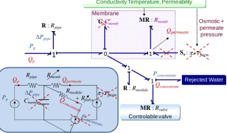
The desalination device involves several power losses in pipes (with its restriction Rpipe), RO membrane, and in the controllable rejection valve (with variable restriction Rvalve) at the output of the rejected salted water. This process is an example of multidisciplinary device coupling chemical, thermal and hydraulic flows (Turki et al., 2008). However, in order to achieve the energy management of the whole system,

a reduced ‘full hydraulic’ model can be extracted in which the membrane is composed of a C element (usually also neglected) and a R variable phenomenon (Rmemb) depending on the membrane conductivity. The feed flow is then shared between the fresh water flow (i.e; the permeate Qpermeate) and the rejected water (i.e; the concentrate Qconcentrate). In our case, we consider brackish water with very small concentration so its osmotic pressure is neglected. A dynamic equivalent hydraulic circuit and its corresponding Bond Graph are displayed in Fig. 3.

1 0

Pp

Qp

Pconcentrate Conductivity Temperature, Permeability

Qpermeate MR : Rmemb C:Cmemb R : Rpipe R : Rmodule 1 1 1 Se:π+Pperm Qconcentrate Controlable valve Membrane Osmotic + permeate pressure MR : Rvalve Pp Qp Rpipe Rmemb Cmemb Qpermeate perm P + π Rmodule + Rvalve Rejected Water ∆Ppipe ∆Ppipe

Fig. 3. Equivalent hydraulic circuit and BG of RO module. From this dynamic BG, a quasi static model of the RO module can be expressed, neglecting the storage effect in

Cmemb (due to the high ‘stiffness’ of the membrane) and the output pressures of permeate and concentrate circuit:

2

)

( module valve concentrate

pipe p P R R Q P −∆ = + (1) membrane pipe p permeate R P P Q = −∆ (2) e concentrat permeate p Q Q Q = + (3)

where Pp, Qconcentrate, Qpermeate, Qp are respectively the output pressure of the high pressure pump , the flow of the rejected water (concentrate), the flow of the fresh water (permeate), and the input flow feed from the pump.

2.2. The pump model

In the same way, a dynamic BG model can be established for the centrifugal pump (see Fig. 4). In this model Pp, Tm, Ω, Qp, are respectively the output pressure and flow of the pump, the motor torque and speed. The mechanical−hydraulic power conversion is modeled by a nonlinear gyrator (see Eq. 4,5) with a and b coefficients (Turki et al., 2008).

Motor 1 _MGY 1 Se : ∆Po Qp R : fm+fp Pp R : c I : Jm+Jp Tm Ω a.Ω b.Qp

Fig. 4. BG of the centrifugal pump

During the pump operation, some losses and dynamic effects appear because of the suction pressure (∆P0), hydraulic

(4)

(Jp + Jm, fp + fm) (Gülich, 2008). By neglecting the Jp + Jm equivalent inertia effect, the static part of the motor-pump model can be expressed as:

) ( ) (a bQ cQ2 P₀ P_p = Ω+ _p Ω− _p+∆ (4) Ω + + + Ω =( p) p ( m p) m a bQ Q f f T (5)

The pump parameters (a, b, c, fm + fp, ∆P0) can be extracted

from experiments or from manufacturer data sheets. 2.3. The pipe model

The pressure drop in the pipe is composed of dynamic and static pressure (Gülich, 2008):

gh KQ P

P

P_pipe = _dynamic+ _static= _p+ρ

∆ 2 ₍₆₎

h being the height of water pumping and ρ the water density.

2.4. The DC equivalent motor model

Classically, centrifugal pumps are driven by Field Oriented Controlled (FOC) inverter fed induction motors (Sul, 2011). If only the energetic behavior is concerned in order to optimize the system management strategy, a simplification should be to consider an equivalent chopper fed DC machine of which parameters are calculated to set the equivalence with the induction motor drive. Then, a BG of this converter motor device can be obtained while simple motor equations are established for the quasi static model by neglecting the motor inertia: Ω Φ + = m m m m R I V (7) m m m I T =Φ (8)

where Tm and Ω are respectively the motor electromagnetic torque and the rotation speed, Φm is the torque equivalent coefficient, Rm is the stator resistance. Then, the electrical power Pe can be expressed from (7) and (8) as:

m m m m m m m m e T T R I V P Φ       Ω Φ + Φ = = (9)

2.5. Whole system modeling

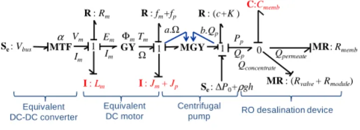
Finally, for the case of the RO subsystem with the HP pump, the whole dynamic BG model is displayed in Fig. 5 in which several series connected elements have been merged as for pump and pipe’s R elements and effort sources. Note that the model is nearly the same for pumping subsystems, except of the hydraulic load which slightly differs.

a.Ω b.Qp R : (c+K ) 1 MGY 1 R : fm+fp Se: ∆P0+ρgh Tm I : Jm+ Jp GY 1 R : Rm I : Lm Em Im Φm MTF Vm Im Se : Vbus α 0 Qp Qpermeate MR: Rmemb C:Cmemb Qconcentrate MR : (Rvalve+ Rmodule) Equivalent DC-DC converter Equivalent DC motor Centrifugal

pump RO desalination device

Ω

Pp

Fig. 5. BG of the whole system

The global static model can be established by neglecting I and C dynamic elements (in red color). In case of pumping operation with no hydraulic load, the motor-pump speed Ω can be derived from (4) and (6) by choosing the positive root of the 2nd order equation:

a gh P Q K c a bQ bQ Q_p p p p 2 ] ) [( 4 ) ( ) ( 0 2 2₊ ₊ ₊_∆ ₊_ρ + − = Ω (10)

The motor torque Tm can then be expressed versus the pump flow Qp from (5) and the electrical power Pe (system input) can be found from (9).

Similarly, in case RO desalination, the pump pressure Pp can be expressed versus the pump flow Qp considering the hydraulic load defined by (1), (2), (3), and (6). A nonlinear expression of the electrical power Pe versus Qp is found by combining (4), (5) and (9).

3. CHARACTERIZATION OF DYNAMIC AND STATIC MODELS

The static model strongly reduces the simulation time for such system. This model reduction is all the more important than an optimization approach is necessary for the power dispatching strategy. In this case, several system simulations have to be performed to reach an optimum value. The dynamic model of Fig. 5 is implemented in the 20-Sim BG solver. The quasi static model is coded in Matlab software. Equation (9) can be inversed by using the “fsolve” function for calculating the pump flow versus the input electrical power. In order to compare the dynamic and quasi-static models, the simplified structure of Fig. 6 is proposed with a well pump and a high pressure pump for desalination.

Pump P1 RO Module Pump P2 Tank T1 Tank T2

Fig. 6. System configuration for BG/static model comparison All tests are based on two pumps from Grundfos:

- The pump P1 (well pump) is rated at 1.5 kW (type SP 5A-17): to feed water to the T1 tank,

- The pump P2 (HP pump for RO) is rated at 2.2 kW (type SP 5A-25) to increase the pressure from T1 to T2 through the RO module. The RO module includes one element (TM710) from TORAY with one pressure body (PV-3110).

Table 1. Grundfos pump parameters

Pump Parameters P1 (SP 5A-17) P2 (SP 5A-25)

a (Ns2/m2) 10.87 13.74

b (Ns2/m5) -6251 -20010

c (Ns2/m8) 1.839×1011 2.193×1011

fm + fp (Nms) 0.0043 0.0050

∆Po (N/m2) 2124 14200

Table 2. The RO module parameters Rmemb (Ns/m5) 1.695.1010

Rmodule (Ns2/m8) 1.038.1012

(5)

The initial level of both tanks (T1 and T2) is 0.2 m. The input power (see Fig.7) is distributed into two equal parts to both pumps (i.e 50% of power sharing factor).

0 50 100 150 200 250 300 0 1 2 3 4 Time (s) In p u t P o w e r (k W ) 1st_transient 4th_transient

Fig. 7. Input power used for model comparison

60 60.2 60.4 60.6 60.8 4.5 5.5 x 10-4 F lo w ( m 3 /s ) Time (s)

Static Model BG Model

Pump P1 60 60.2 60.4 60.6 60.8 2.5 3 x 10 -5 Time (s) Pump P2

F lo w (m 3 /s ) 60 60.2 60.4 60.6 60.8 0.25 0.50 E ff ic ie n cy

Pump P2 Pump P1

Time (s)

Fig. 8. Difference between models during the 1st transient

0.9 1.5 x 10 F lo w ( m 3 /s ) 240 240.2 240.4 240.6 240.8 -3 Pump P1

Time (s) 240 240.2 240.4 240.6 240.8 6 9 x 10-5 F lo w (m 3 /s ) Time (s) Pump P2

240 240.2 240.4 240.6 240.8 0.15 0.55 E ff ic ie n cy Pump P2 Pump P1

Time (s)

Fig. 9. Difference between models during the 4th transient The resulting difference between both dynamic and quasi static models is not significant in terms of power/energy balance over a wide range of operation. A small difference only occurs at transients as illustrated in Fig. 8 and Fig. 9 (note that results are also the same for second and third transients). Finally, the reduced quasi static model is considered as acceptable in order to optimize the system management which allows reducing significantly the convergence time of optimization as presented in the next section.

4. WATER MANAGEMENT STRATEGY 4.1. Setting the problem of water management

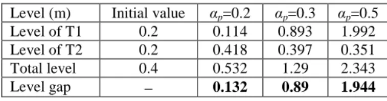
This section sets the problem to be solved in order to simultaneously manage power and water flows with a maximum efficiency during the system operation. We still use the simplified configuration as in Fig. 6 with the input power of Fig. 10. We show in Fig. 11 and in Table 3 the water level stored in both tanks when this power is dispatched according to different power sharing factor αp defined as: 2 1 1 1 e e e in e p P P P P P + = = α (11)

where Pe1 and Pe2 denotes the electrical powers feeding respectively the pump P1 and the pump P2, Pin is the input power to be dispatched. It can be seen from Table 3 and Fig. 11 that different water levels can be obtained in each tank according to the αp value. In the first case (αp = 0.2), the increase of total level is the smallest because the pump P1 operates in the region of low efficiency with very low input power. This example emphasizes the first coupling between power and subsystems efficiency: the generated power from renewable sources is then strongly coupled with the water process system efficiency. In particular, the importance of respecting pumping power limits to prevent problematic operations that degrade efficiency and that could also reduce the life duration of pumps. The last case (αp = 0.5) gives the best result because both pumps operate with good efficiency.

0 500 1000 1500 2000 2500 1.4 1.6 1.8 P o w e r (k W ) Time (s)

Fig. 10. Input power used for showing the influence of the energy management based on power dispatching

Pe1 Pe1 Q1 η1 η2 η1 Q1 Pe2 Q2 η2 Pe2 Q2 Pe1 Q2 η2 η1 Q1 Pe2 L2 L2 L1 L1 L2 L1 (Initial) L2 L1 α p=0.2 α p=0.3 α_p=0.5 α p=0.2 αp=0.3 αp=0.5

(a) Operating points: efficiency (η) and flow (Q) (b) Water levels

Fig. 11. Water levels obtained from various operating points corresponding to different power sharing factors

Table 3. Tank levels for different power sharing factors

Level (m) Initial value α_p_=0.2 α_p_=0.3 α_p_=0.5

Level of T1 0.2 0.114 0.893 1.992 Level of T2 0.2 0.418 0.397 0.351 Total level 0.4 0.532 1.29 2.343 Level gap − 0.132 0.89 1.944

(6)

Note that this result is only related to a particular sizing of the two pumps (here respectively 1.5 and 2.5 kW). Modifying its sizing should also vary the system performance: this latter issue emphasizes the second coupling between sizing and management performance. A third coupling, between tank level and power management has also to be managed: indeed, after a certain operation time, the maximum level of tanks can be attained. On the opposite, operating the pumps P2 is only possible if the tank T1 is not empty. Based on this strongly coupled system design (water management and pump sizing), the next subsection aims at optimizing the operation and especially the power dispatching strategy. 4.2. Formulation of the optimal power dispatching

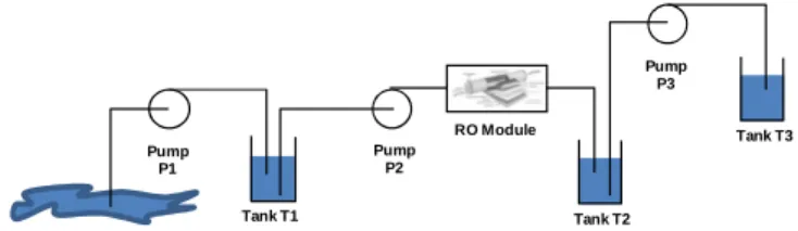
In the following, we will consider a more complete system with 3 pumps, corresponding with the synoptic of Fig.1 and displayed in Fig. 12. All tanks have the same volume with a base area of 1 m2 and a height of 2 m. The initial level of all tanks is set at: 1m for T1, 0.2 m for T2 and 0.2 m for T3.

Pump P1 RO Module Pump P2 Tank T1 Tank T2 Pump P3 Tank T3

Fig. 12. Desalination system base on RO module

The input power is sampled every 10 min. At each sample, a dispatching algorithm is performed in order to share the input power between all pumps, while ensuring operating constraints: in particular, the shared power assigned to each pump has to be bounded by pump technological limits (i.e.

Pemin ≤ Pe ≤ Pemax) and the level L in each tank has to lie in the interval Lmin ≤ L ≤ Lmax corresponding to the capacity

limits. Each of the three pumps having two possible operating states SP (i.e. SP = 1 or SP = 0 respectively for on/off operations), eight possible states S=SP3SP2SP1 are a priori feasible at every sampling period (from S = 000 to S = 111). The dispatching algorithm first identifies the number of possible states, i.e. which pump can be switched according to the input power range conditions and to the current levels of the tanks. For example, if the tank T3 is full, the pump P3 has to be switched off and only four states are feasible (from

S = 000 to S = 011). Then, for each feasible state a second

step is performed consisting in optimizing the input power dispatching. The optimal dispatch problem can be formulated into the following constrained optimization problem:

      ≤ ≤ ≤ ≤ = = = 3 .. 1 max min 3 .. 1 max min , , ) ( max 3 2 1 i i i i i ei ei ei obj Q Q Q L L L P P P f p p p x x (12)

where the objective function to be maximized should represent the efficiency of the energy and flow transfers in the system. Such problem can be solved using standard nonlinear programming methods (typically by means of

fmincon Matlab function). Note also that pump flows Qpi are

used for the decision variables instead of the corresponding shared electrical power Pei in order to avoid the inversion

of (9). Each feasible state leads to an optimal objective function and the best value obtained among all states is returned. The corresponding power values for switched on pumps are considered as power references. In this particular problem, the choice of the objective function is not obvious. Indeed the issue is to minimize the time needed to fill the superior tank T3. Then, given a certain input power fed by the renewable intermittent sources, the power dispatching strategy has to pay attention of energy efficiency of the three pumps but also of the tank levels: five different objective functions are proposed and compared in the next subsection. 4.3. Proposed objective functions for the dispatching strategy The f1 objective function deals with the system efficiency:

in i pi pi in i hydraulics in out P Q P P P P P f

∑

= = ₌ = = 3 1 3 1 1 (13)

The f2 objective function aims at maximizing the total flow:

∑

= = 3 1 2 i pi Q f (14)

The f3 objective function is the same as f3 but with weighting

coefficients depending on the tank level:

∑

= = 3 1 3 i pi iQ f ω where min max max i i i i i L L L L − − = ω (15)

The f4 objective function is similar to f3 but with quadratic

flows:

∑

= = 3 1 2 4 i pi iQ f ω (16)

Finally the f5 objective function aims at maximizing the

output hydraulic powers as for f1 but with weighting

coefficients ωi linked with tank levels similarly to (15):

∑

= = = = 3 1 3 1 5 i pi pi i i hydraulics iP P Q f ω ω (17)

The proposed objective functions need to be tested with different input power waveforms. The criterion to compare the objective function robustness is the “finishing time”, that means the time needed to fill the three tanks T1, T2 and T3 (with 2 m of height for everyone) from an initial level of 1 m for T1, 0.2 m for T2 and 0.2 m for T3.

4.4. Results and analysis

All tests have been applied with three waveforms of input power. Time (s) 4 4.2 4.4 4.6 x 104 0 3 6 9

Triangle (A) Guadeloupe (B) Tun isia (C)

In te rm it te n t I n p u t P o w e r (k W ) 20 min

(7)

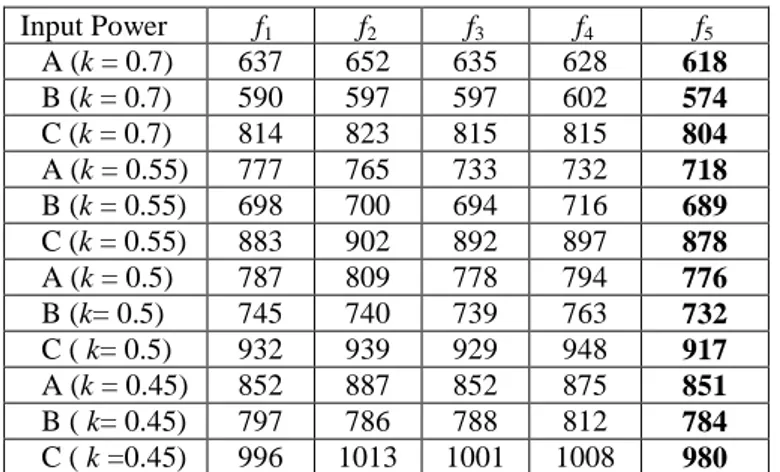
The first waveform (A) is for an input power with a theoretical triangle shape. The second waveform (B) corresponds to an intermittent power issued from wind turbine measurements in Guadeloupe (with small sampling period). Similarly, the third waveform (C) is relative to a power cycle extracted from wind turbines in Tunisia (with higher sampling period). In the following, the amplitude of the input power waveform is multiplied by several reduction factors k varying from 0.45 to 0.7 in order to analyze the coupling between the system environment (i.e. the shape and the amplitude of the given input power) and the system efficiency. It can be observed from Table 4 that the most appropriate objective function is f5 (column in bold type in

Table 4) which corresponds to the maximization of the output power weighted with the level of the tanks. This objective function can also be considered as robust versus input profiles as it always offers the smallest finishing time whatever the power waveform and its reduction factor k.

Table 4. Finishing time (in min) for different objective functions Input Power f1 f2 f3 f4 f5 A (k = 0.7) 637 652 635 628 618 B (k = 0.7) 590 597 597 602 574 C (k = 0.7) 814 823 815 815 804 A (k = 0.55) 777 765 733 732 718 B (k = 0.55) 698 700 694 716 689 C (k = 0.55) 883 902 892 897 878 A (k = 0.5) 787 809 778 794 776 B (k= 0.5) 745 740 739 763 732 C ( k= 0.5) 932 939 929 948 917 A (k = 0.45) 852 887 852 875 851 B ( k= 0.45) 797 786 788 812 784 C ( k =0.45) 996 1013 1001 1008 980

5. INFLUENCE OF THE PUMP SIZING ON THE SYSTEM EFFICIENCY

This section aims at analyzing the coupling effect between sizing and system management. Only the most robust objective function f5 is used in that part in order to test

different combinations of motor pump sizing. These combinations include electrical converters, electrical motors and pumps. Several combinations with rated powers from 1.5 kW to 11 kW are displayed in Table 5. Only the waveform C of the input power from Tunisia with three different reduction factors k is considered.

Table 5. Finishing time (in min) for different sizing

Rated powers of P1, P2, P3* C k = 0.7 C k = 0.55 C k = 0.5 (1.5 kW 1.5 kW 1.5 kW) 914 965 985 (1.5 kW 2.2 kW 1.5 kW) 804 878 917 (1.5 kW 4.0 kW 1.5 kW) 801 898 879 (1.5 kW 7.5 kW 1.5 kW) 757 827 886 (1.5 kW 11 kW 1.5 kW) 748 840 938 *

Reference of used pumps from Grundfos manufacturer: 1.5kW– SP5A-17; 2.2kW – SP5A-21; 4kW – SP5A 44N; 7.5kW – SP 5A 75; 11kW – SP8A 73.

Best results (i.e. the smallest finishing time) are indicated in bold type in this table. As we can observe, it is necessary to investigate the sizing of the three pumps combination to get an optimal system design. It is interesting to note that the smaller the amplitude of input power (i.e. when k decreases), the smaller the optimal rated power for the combination of pumps. It should also be noted that there is a strong coupling between sizing and environment profile (i.e. shape and intensity of the input power).

6. CONCLUSIONS

In this paper, the energy management of a water pumping and desalination process has been studied. Based on a quasi static model validated with a dynamic BG model, an optimal dispatching strategy has been proposed for sharing the intermittent input power between different pumps. In particular, the choice of the objective function used in this strategy for assessing the operating efficiency has been analyzed. It is shown that a robust solution consists in taking as objective function the sum of hydraulic powers weighted by the associated tank levels. On the other hand, the influence of the pump sizing on the system efficiency is also underlined. This justifies new studies in order to investigate global optimization approaches taking account of the couplings between the system architecture, sizing and energy management.

REFERENCES

Ben Rhouma A. Belhadj J., Roboam X. (2008). Control and energy management of a pumping system fed by hybrid Photovoltaic-Wind sources with hydraulic storage.

Journal of Electrical Systems, Vol. 4, 1−16.

Charcosset C. (2009). A review of membrane processes and renewable energies for desalination. Desalination, Vol. 245, 214–231.

Dali M., Belhadj J., Roboam X. (2009). Hybrid wind-photovoltaic power systems: Structure Complexity and Energy Efficiency, Control and Energy management.

EJEE RIGE, Vol. 12, 669–700.

Gülich. J.F. (2008). Centrifugal Pumps, 964. Springer, Verlag Berlin Heidelberg, New York.

Kalogirou. S. A. (2005). Seawater desalination using renewable energy sources. Progress in Energy and

Combustion Science, Vol. 31, 242–281.

Karnopp D., Margolis D., Rosenberg R. (2006), System

Dynamics: Modeling and Simulation of Mechatronic Systems, 563. John Wiley & Sons, Hoboken.

Koklas P.A., Papathanassiou S.A. (2006). Component sizing for an autonomous wind-driven desalination plant.

Renewable Energy, Vol. 31, 2122–2139.

Sul S. K. (2011). Control of Electric Machine Drive System, 399. John Wiley & Sons, Hoboken, New Jersey.

Tanaka, K., Rong, W., Suzuki, K., Shimizu, F., Hatakenaka, K., and Tanaka, H., (2000) Detailed Bond Graph of Turbomachinery. IEEE IECON, 1550–1555.

Turki M., Belhadj J., Roboam X., (2008). Control strategy of an autonomous desalination unit fed by PV-wind hybrid system without battery storage. Journal of Electrical