To cite this document:
Bolting, Jan and Defaÿ, Francois and Moschetta, Jean-Marc
Differential GPS for small UAS using consumer-grade single-frequency receivers. (2013)
In: International Micro Air Vehicle Conference and Flight Competition (IMAV2013), 17
September 2013 - 20 September 2013 (Toulouse, France).
O
pen
A
rchive
T
oulouse
A
rchive
O
uverte (
OATAO
)
OATAO is an open access repository that collects the work of Toulouse researchers and
makes it freely available over the web where possible.
This is an author-deposited version published in:
http://oatao.univ-toulouse.fr/
Eprints ID: 10619
Any correspondence concerning this service should be sent to the repository
administrator:
[email protected]
Differential GPS for small UAS
using consumer-grade single-frequency receivers
Jan Bolting
1, Francois Defa¨y
2and Jean-Marc Moschetta
21 University of Braunschweig - Institute of Technology, Braunschweig, Germany
2 Institut Supérieur de l’Aéronautique et de l’Espace, Toulouse, France
[email protected], [email protected] Abstract
Consumer-grade single-frequency GPS receivers with their known limitations are the predomi-nant means of localization for small Unmanned Aircraft Systems (UAS). More intricate maneuvers such as automatic landings require a level of accuracy this class of receivers does not provide. As a contribution to improve the positioning accuracy without sacrificing the low-cost approach of this class of vehicles, a Local Area Augmentation System (LAAS) has been developed, based on consumer-grade single-frequency miniature GPS receivers both for the base station and airborne positioning.
On the part of the airborne receiver, the conventional approach of carrier phase smoothing has been extended by incorporating Doppler measurements to propagate the position during carrier phase signal outages or in the event of cycle slips. Pseudoranges and the augmented carrier phase observations are merged by means of an indirect linear Kalman filter in the position domain. The characteristics of the error state allow for some simplifications that reduce the computing effort of the filter.
To evaluate the system’s performance under dynamic conditions, raw GPS data have been collected on a ground based moving platform and processed with Simulink. The results show a significantly improved 3D position accuracy compared to the standalone receiver solution.
Contents
1 Introduction 2
2 Observations of a GNSS receiver 2
3 Base station 3
3.1 Base station positioning . . . 4
4 Airborne positioning algorithm 4
4.1 Background Trajectory . . . 5 4.2 Absolute positioning . . . 6
5 Experimental results 7
5.1 Base positioning . . . 7 5.2 Dynamic tests on the ground . . . 7
1
Introduction
Progress in low-cost sensor and computing technology within the last years has led to a growing num-ber of new low-cost UAS designs for civil applications. Typically, they rely on single-frequency GPS receivers for localization due to their low-cost profile. Despite the efforts of manufacturers to improve the accuracy of single-frequency receivers by better modeling of atmospheric effects and the availabil-ity of space based augmentation systems such as EGNOS, today’s low cost receivers are limited to 3D positioning errors of the order of several meters (1 σ). This is adequate for cruise flight navigation but is expected to be a severe constraint for enlarging the flight envelope of small UAS including more advanced maneuvers such as automatic takeoffs and landings in confined areas and formation flight of multiple UAS.
In civil and military aviation, Ground Based Augmentation Systems (GBAS) are used to enhance the accuracy of GNSS positioning to a level that, for instance, allows fully automatic approaches. Unfortunately, commercial differential GNSS receivers do not meet the cost requirements of small UAS for civil applications. There are however low-cost receivers on the market that output raw code, carrier phase and Doppler observations and are thus in principle suitable for differential positioning techniques. This has been the motivation to investigate the achievable accuracy of a ground based augmentation system for UAS based on low-cost consumer-grade receivers.
There have been efforts before to use inexpensive single-frequency receivers for kinematic precise po-sitioning applications, mostly for popo-sitioning of ground vehicles, see e.g. [4], [7]. The authors of [9] use L1 phase observations collected with a u-blox LEA-4T for the reconstruction of relative flight trajectories and obtain positive results using time-differenced carrier phase observations.
Precise absolute positioning with low cost single-frequency receivers is challenging compared to dual-frequency navigation grade receivers that are routinely used for surveying applications. Their observa-tions typically exhibit a higher noise level, degrading the accuracy of the code based position and thus enlarging the search space for carrier ambiguity resolution. Since the ionospheric range error cannot be eliminated by forming the ionosphere-free combination of the two signals, corrections are valid only for up to about 10 km. In addition, they lack the advantage of accelerated ambiguity resolution by means of the wide-lane combination of the two carrier phase observations.
Embedded systems on board of small UAS are typically based on sub - GHz microcontrollers due to power and size constraints, thus a positioning system that requires low computing power is desirable. Moreover, continuous availability of a position estimate is of the essence to ensure operational safety. This article describes an approach towards meeting these two requirements. Results are given of a first implementation of the augmentation system in Matlab/Simulink. It has been applied to raw data collected on a ground based moving platform.
The article is organized as follows: after introducing the observation model in section 2, section 3 presents the computation of broadcast corrections and the method that is proposed to obtain the reference station position, section 4 is devoted to the positioning algorithm of the airborne receiver. Finally, section 5 presents our experimental results and section 6 gives a short summary and an outlook on future work.
2
Observations of a GNSS receiver
A GNSS receiver’s pseudorange, carrier phase and carrier Doppler shift observations are commonly modeled as
ρi= ri+ c(∆trx+ ∆tSV,i) + ∆rion,i+ ∆rtrop,i+ ∆reph,i+ ∆rM P,ρ,i+ ∆rHW,ρ,i (1) Φi= ri+ c(∆trx−∆tSV,i) − ∆rion,i+ ∆rtrop,i+ ∆reph,i+ λiNi+ ∆rM P,Φ,i+ ∆rHW,Φ,i (2) vDo,i= ˙rRx,i+ c( ˙∆trx−∆tSV,i˙ ) −∆rion,i˙ +∆rtrop,i˙ +∆rM P,Φ,i˙ +∆reph,i˙ + ∆vHW,Do,i (3) with
˙rRx,i= ˙ri−˙rSV,i
where ρi is the pseudorange observation, ri the slant range according to the broadcast ephemeris, c the nominal speed of light used by the GNSS system, ∆trx the receiver clock offset, ∆tSV,i the satellite clock offset, ∆rion,i the range error due to ionospheric diffraction, ∆rtrop,i the range error due to tropospheric diffraction, ∆reph,i the line of sight (LOS) broadcast ephemeris error, ∆rM P,ρ,i the range error due to code multipath, Φi the carrier phase range observation, λ the nominal carrier phase wavelength, N the carrier cycle ambiguity, ∆rM P,Φ,icarrier phase multipath, vDo,ithe Doppler shift observation, transformed to a velocity and ˙rRx,i the slant range rate corrected for the satellite’s LOS velocity. Hardware noise is represented by ∆rHW,ρ,i, ∆rHW,Φ,iand ∆vHW,Do,irespectively. ˙rSV,i is the range rate due to satellite motion as computed from broadcast ephemeris.
Differential augmentation systems exploit the fact that a major part of the measurement errors is highly correlated between two receivers that are sufficiently close to one another, due to the fact that the signals they receive experience very similar conditions on their way through the atmosphere. This allows the estimation of the common errors once the position of one receiver - herein referred to as the base station - is known.
3
Base station
The base station consists of a GPS receiver that is placed at a known location and a data processing system that computes the corrections and broadcasts them via a wireless datalink to an unlimited amount of UAS.
Both code and phase observations evolve rapidly in time due to the high orbital velocity of the satellites (affecting ri) and the rapidly drifting clock offset ∆trxof the u-blox receiver’s free running clock. While the latter is common to all observations and thus is eliminated by solving the nav-igation equation, the first imposes hard timing constraints on the data link and the synchronicity of the measurements of the base receiver and the airborne receiver when using a single-differencing approach. Therefore, ri is computed from broadcast ephemerides (see [2]) and subtracted from the pseudorange observations to form estimates of the common range errors. The base receiver’s clock error is not removed from the corrections to avoid increasing the variance of the corrections. Thus the pseudorange corrections are formed as
ρc,i= c(∆trx+ ∆tSV,i) + ∆rion,i+ ∆rtrop,i+ ∆reph,i+ ∆rM P,ρ,i+ ∆rHW,ρ,i (4) The phase observations are treated in the same way, forming carrier phase corrections:
Doppler corrections are obtained by time-differencing of carrier phase corrections.
Note that due to the fact that the broadcast ephemerides are only local approximations of the satellite orbits, it has to be made sure that the base station and the airborne receiver use the same set of ephemerides.
3.1
Base station positioning
It will seldom be the case that a surveyed reference point is available for the base station. Conse-quently, a way has to be found to estimate its position in a reasonable amount of time. An error of the base position directly translates into an additional position offset of receivers using its corrections, thus the quality of the ground station positioning determines the achievable accuracy for the UAS. The International GNSS Service (IGS) provides observation data of a worldwide network of GNSS ref-erence stations. A subset of these stations provide their data in close-to-real-time via NTRIP streams. Tests have been run and it could be demonstrated that, using the open-source RTK positioning soft-ware rtklib, the base receiver position can be computed with sufficient accuracy within 20 minutes, provided there is a reference station that is sufficiently close. Please see section 5.1 for experimental time-to-ambiguity-resolution results for three baselines up to 134 km.
4
Airborne positioning algorithm
The airborne component applies the received corrections to its own observations, canceling the major part of common errors, leading to the corrected observations
ρi,c= c∆trx,c+ ∆rM P,ρ,i+ ∆rHW,ρ,i,c+ ǫ∆rρ,c (6) Φi,c= c∆trx,c+ λNc+ ∆rM P,Φ,i+ ∆rHW,Φ,i,c+ ǫ∆rΦ,c (7)
vDo,i,c= c ˙∆trx+ǫ∆r˙Φ,c+ ∆vHW,Do,i,c+ ǫ∆rDo,c (8)
where ∆trx,cis the difference of the clock offsets of base and airborne receiver, Nc the difference of their integer ambiguities, ∆rHW,ρ,i,c,∆rHW,Φ,i,cand ∆vHW,Do,i,c the combined noises of observations and corrections. Residual common errors due to timely and spatial de-correlation are represented by ǫ∆rρ,c, ǫ∆rΦ,c and ǫ∆rDo,c.
The UAS position is obtained in two steps. First, a relative trajectory based on carrier phase time differences and integrated Doppler observations is computed. Second, the absolute position is obtained from pseudoranges and both are merged by an indirect Kalman Filter. Both steps are described in more detail in the following sections.
Position domain code smoothing is superior to range domain approaches under dynamic conditions for two major reasons: First, three coordinates to be estimated instead of up to e.g. about seven ranges for GPS leads to smaller filter matrices and thus reduces execution time.
Second, and more importantly, in the range domain, after loss of lock and reacquisition of a satellite, its smoothed range is lost and the respective filter channel is re-initialized. Afterwards, the smoothed range will be unusable while the filter re-converges. This can be impractical if less than 4 converged ranges are available, forcing the rover to use a range being still in the convergence phase and leading to a degraded position estimate.
On the other hand, in the position domain only an arbitrary set of four or more range and delta range observations has to be available at all times to keep up a continuous smoothed position. A reacquired satellite can be used immediately for positioning. This is a particularly valuable property
in urban environments. Imagine an airborne rover that subsequently looses lock to all satellites for a few epochs, but manages to maintain a set of 4 satellites all the time. If the rover uses a range domain filter, it is left with a set of filtered ranges whose error is thrown back to that of their pseudorange measurements. A position domain filter might experience an increased noise level due to a higher PDOP associated with fewer satellites in view, but run continuously.
4.1
Background Trajectory
Numerous approaches exist to solve for the unknown integer ambiguities to obtain a highly accurate purely carrier phase based position. Most of them are search-based (e.g. LAMBDA, introduced by [8] ), but there are promising analytical approaches for On-The-fly ambiguity resolution as well, e.g. [3]. There is no known technique that provides reliable and instantaneous ambiguity resolution for L1-only receivers though. The author of [5] shows, based on theoretical considerations, that at least 12 satellites in view are necessary for on-the-fly ambiguity resolution in 100% of all cases, a condition that is not met by the GPS constellation.
A simple alternative to exploit the excellent accuracy of carrier phase measurements without the need for ambiguity resolution consists in time-differencing. Since for a continuously tracked signal the am-biguities are constant in time, they are canceled by subtracting the observations of two subsequent epochs. The method has been successfully applied to standalone L1 phase observations for the analysis of flight maneuvers of aircrafts and birds (see [10], [11]).
As every technique involving phase observations, this method is susceptible to cycle slips and loss of the carrier signal. In situations where - e.g. due to steep maneuvers - the number of available phase observations drops below four, the accurately tracked trajectory is lost.
To overcome this drawback, the method has been extended by incorporating integrated Doppler ob-servations that are less susceptible to dynamic stress, leading to better availability. Whenever the number of available carrier phase time differences drops below the minimum of four, they are aug-mented by integrated Doppler observations, i.e.
δr = δrcp,1 .. . δrcp,ncp for ncp ≥4 (9) δr = δrcp,1 .. . δrcp,ncp δrDo,1 .. . δrDo,(ncp−4) for ncp <4 (10) with δrDo,i= Z tk tk−1 vDo,idt (11)
δrcp,i are carrier phase time differences, δrDo,i are integrated Doppler delta ranges of satellites whose carrier phase time differences are not available and ncp represents the number of available carrier phase time differences.
Doppler observations are a snapshot of the derivative of the trajectory, i.e. the velocity, at the time of measurement. Their integral therefore only approximates the true displacement and integrated Doppler ranges are noisier than carrier phase ranges. The advantage of not loosing track of the tra-jectory however largely outweighs this drawback, the more so as integrated Doppler observations are only used during the short periods of carrier phase outages.
The position increment between two epochs is calculated by linearizing the observation equation (here given for one range, note that δri,k represents the carrier phase time differences augmented by integrated Doppler delta ranges)
δri,k= q (xSV k −xRxk )2+ (ySVk −ykRx)2+ (zSVk −zkRx)2 − q (xSV k−1−xRxk−1)2+ (ySVk−1−yk−1Rx )2+ (zk−1SV −zk−1Rx )2 (12) +c(∆tRx,k−∆tRx,k−1) + (ǫk−ǫk−1) and by solving it iteratively for xk by the method of least squares.
4.2
Absolute positioning
Based on the corrected pseudoranges, the absolute position is computed following the standard proce-dure of linearizing and iteratively solving the navigation equation. To correct for the signal propagation delay, pseudoranges are time-tagged at the receiver, as proposed by [1]. The resulting noisy position estimate is used to correct the position offset of the background trajectory by means of a simple linear Kalman filter.
The prediction-correction structure of a Kalman Filter usually requires a dynamic model of the system whose state is to be estimated and knowledge about the control inputs. In this case, the offset of the background trajectory from the true trajectory drifts very little over time thanks to its excellent relative precision. It can therefore be approximately modeled as being constant, i.e the dynamics matrix A ≈ I3 which is equivalent to omitting the state prediction step.
This naturally leads to an indirect i.e. error state filter formulation, as the difference between the pseudorange trajectory and the background trajectory is a noisy measurement of the background trajectory offset. The filter equations become
∆xk = xb,k−∆xtrue,k (13) ∆ˆx− k = A∆ˆxk−1 (14) P− k = APk−1AT+ Q (15) ∆zk = xρ,k−xb,k (16) Kk = P−k(P−k + R)−1 (17) ∆ˆxk = ∆ˆx−k + Kk(∆ˆxk−∆zk) (18) Pk = (I − Kk)P−k (19)
∆xk being the error state, ∆zk being the error state measurement, Kk being the filter gain, ∆ˆx−k, ∆ˆxk being the a priori and a posteriori error state estimate respectively, P−k, Pk being the a priori and a posteriori estimation covariance matrix respectively, Q being the process noise and R being the measurement noise.
5
Experimental results
The system has been implemented in Matlab/Simulink and applied to observations collected on a rotating test bench on the ground. Flight tests have been performed as well but are not considered in this article since no RTK trajectory could be obtained in post processing. Base positioning using freely available close-to-real-time observations by the IGS network ([6]) has been tested for three baseline lengths up to 134 km.
Hardware Data have been collected with GPS receivers of type u-blox LEA-6T. The LEA-6T chipset is one of the least expensive on the market providing raw observations on the GPS L1 band. Receiver modules integrating the same receiver chip as the evaluation kit used for our experiments are available with a weight of 16g including an active antenna, making them suitable for small UAS down to a few hundred grams TOW. The rover and base antennas where an active patch antenna (u-blox ANN-MS-0-005) and a survey grade antenna on a surveyed reference position, respectively.
5.1
Base positioning
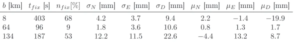
To verify the assumption that the position of the base receiver can be determined in a reasonable amount of time using freely available reference observations and open source software, tests for three successively large baselines have been performed. Data have been collected for 20 minutes and pro-cessed with rtklib. The positions obtained by averaging all positions with fixed ambiguities are of centimeter-level quality (see Table 1), better accuracy can be expected for longer sampling periods. Longer baselines have been tested but did not lead to fixed ambiguities within 20 minutes.
b[km] tf ix [s] nf ix[%] σN [mm] σE [mm] σD[mm] µN [mm] µE [mm] µD [mm]
8 403 68 4.2 3.7 9.4 2.2 −1.4 −19.9
64 96 9 1.8 3.6 10.6 0.8 1.3 1.7
134 187 53 12.2 11.5 22.6 −4.4 13.2 8.7
Table 1: LEA-6T base positioning with rtklib for different baselines (stations TLMF, PAYR, NARB). tf ix is the time when ambiguities where fixed for the first time, nf ix the percentage of epochs for which ambiguities could be fixed within 20 minutes.
5.2
Dynamic tests on the ground
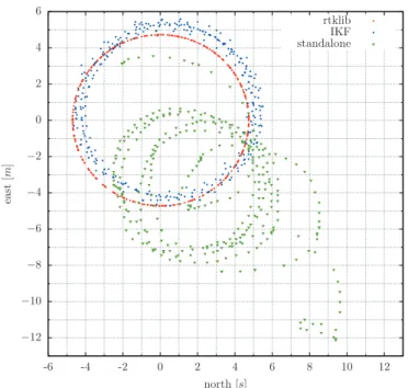
To emulate flight conditions, the receiver has been placed on a freely rotating turntable with a radius of 4.2 m. As with all localization systems, a key challenge consists of the comparison of measurements from the system to be tested versus a known truth source. In this case the true trajectory could be reconstructed with RTK-level accuracy using the open-source software rtklib (see e.g. [7]). The bar
−12 −10 −8 −6 −4 −2 0 2 4 6 -6 -4 -2 0 2 4 6 8 10 12 east [m ] north [s] rtklib IKF standalone
Figure 1: North and east coordinate of trajectory in local NED frame
was rotated by one person. A second receiver was set up to record raw data at the campus’ surveyed reference antenna. In parallel to the raw observations, the standalone position solution of the receiver has been logged. The test site was located 40 to 80 m from two two-story buildings, thus the rover receiver was likely to experience multipath.
The position errors over time are given in Fig. 2, see Fig. 3 and Tab. 2 for error statistics.
While not exceeding 5 m most of the time, the standalone error rises to up to 16 m in the east coordinate around 330 s. The filtered differential solution error stays well close to 1 m most of the time and exhibits a smaller variance. Note also that the filtered solution shows no sign of the two discontinuities at 25 s and 305 s in the receiver’s solution. Regarding the total error (norm of the error vector), for the standalone solution 95 % of all 3D errors are smaller than 11.15 m. The Kalman filtered differential solution brings the 95% error range down to 1.35 m.
σN [m] σE [m] σD [m] µN [m] µE [m] µD [m] HDOP VDOP Circular trajectory, baseline 180 m
standalone 2.18 2.06 1.74 2.67 −4.41 0.74 -
-Differential C/A 0.86 0.65 2.39 0.06 −0.2 −0.47 1.2-1.4 2.1-3.6
IKF 0.21 0.21 0.26 0.38 0.49 −0.85 1.2-1.4 2.1-3.6
Table 2: Position error standard deviations σ and means µ under static and dynamic conditions (300 s, 1 Hz)
−15 −10 −5 0 5 10 15 error north [m ] −15 −10 −5 0 5 10 15 error east [m ] −15 −10 −5 0 5 10 15 0 50 100 150 200 250 300 error do w n [m ] time [s]
IKF C/A standalone
IKF C/A standalone
IKF C/A standalone
Figure 2: Position offset to RTK trajectory in local NED system: indirect Kalman Filter, differential C/A, LEA-6T standalone solution (SBAS enabled, configured for airborne platforms ≤ 4 g)
0
50
100
0
0.4 0.8 1.2 1.6
2
Cum
ulativ
e
probabilit
y
[%]
error [m]
IKF
0
4
8
12 16 20
error [m]
differential C/A
0
4
8
12 16 20
error [m]
standalone
Figure 3: Cumulative distributions of 3D error on circular trajectory. Note the different scales of the x axes.
6
Conclusions and future work
This work has investigated the feasibility of a local GPS augmentation system based on low cost hardware components. A code smoothing filter has been developed that takes advantage of the complementary qualities of carrier phase, Doppler and pseudorange observations, based on an indirect linear Kalman filter. The positioning filter has been implemented in Matlab/Simulink and applied to observation data collected on a rotating test bench. A highly accurate reference trajectory could be reconstructed using open - source RTK post-processing software. The results are quite promising and reveal the shortcomings of standalone dynamic GPS positioning. Differential positioning shows an improvement of the mean position error (the only exception being the vertical error whose mean values are of similar magnitude) as well as the error variance by roughly one magnitude. Further efforts will be focused on the implementation of the proposed system on an embedded system and the verification of its performance under flight conditions, including the tracking of the reference trajectory by means of GPS-independent instruments such as theodolites to exclude the possibility of common errors. Its robustness thanks to the integration of Doppler measurements makes the proposed system an excellent basis and safety fall-back for the evaluation of more accurate but less reliable techniques involving ambiguity resolution.
References
[1] Neil Ashby and Marc Weiss. NIST Technical Note 1385 "Global Position System Receivers and Relativ-ity". Technical report, United States National Institute of Standards and Technology, 1999.
[2] Interface Control Working Group. Global Positioning System Interface Specification IS-GPS-200G. Global Positioning Systems Directorate - Systems Engineering & Integration, September 2012.
[3] Xiaogang Gu and A. Lipp. DGPS positioning using carrier phase for precision navigation. In Position Location and Navigation Symposium, 1994., IEEE, pages 410 –417, apr 1994.
[4] Kjeld Jensen, Morten Larsen, Tom Simonsen, and Rasmus N. Jørgensen. Evaluating the performance of a low-cost gps in precision agriculture applications. In RHEA-2012 - First International Conference on Robotics and Associated High-Technologies and Equipment for Agriculture, 2012.
[5] Dennis Milbert. Influence of Pseudorange Accuracy on Phase Ambiguity Resolution in Various GPS Modernization Scenarios. NAVIGATION, 52:29–38, 2005.
[6] International GNSS Service. http://igscb.jpl.nasa.gov/network/netindex.html.
[7] Tomoji Takasu and Akio Yasuda. Development of the low-cost RTK-GPS receiver with an open source program package RTKLIB. International Symposium on GPS/GNSS, 2009.
[8] P. J G Teunissen. A new method for fast carrier phase ambiguity estimation. In Position Location and Navigation Symposium, 1994, IEEE, pages 562–573, 1994.
[9] J. Traugott, G. Dell’Omo, A.L. Vyssotski, D. Odijk, and G. Sachs. A time-relative approach for precise positioning with a miniaturized L1 GPS logger. In Proceedings of ION GNSS 21th International Technical Meeting of the Satellite Division, pages 1883–1894. ION GNSS, 2008.
[10] Johannes Traugott, Dennis Odijk, Oliver Montenbruck, Gottfried Sachs, and Christian Tiberius. Making a Difference with GPS. GPS World, May 2008:48–57, 2008.
[11] Johannes P. Traugott. Precise Flight Trajectory Reconstruction Based on Time-Differential GNSS Carrier Phase Processing. PhD thesis, Technische Unversitaet Muenchen, 2011.