Quaterninic Kähler manifolds, constrained instantons, and the magic square

AVIS

Ce document a été numérisé par la Division de la gestion des documents et des archives de l’Université de Montréal.

L’auteur a autorisé l’Université de Montréal à reproduire et diffuser, en totalité ou en partie, par quelque moyen que ce soit et sur quelque support que ce soit, et exclusivement à des fins non lucratives d’enseignement et de recherche, des copies de ce mémoire ou de cette thèse.

L’auteur et les coauteurs le cas échéant conservent la propriété du droit d’auteur et des droits moraux qui protègent ce document. Ni la thèse ou le mémoire, ni des extraits substantiels de ce document, ne doivent être imprimés ou autrement reproduits sans l’autorisation de l’auteur.

Afin de se conformer à la Loi canadienne sur la protection des renseignements personnels, quelques formulaires secondaires, coordonnées ou signatures intégrées au texte ont pu être enlevés de ce document. Bien que cela ait pu affecter la pagination, il n’y a aucun contenu manquant.

NOTICE

This document was digitized by the Records Management & Archives Division of Université de Montréal.

The author of this thesis or dissertation has granted a nonexclusive license allowing Université de Montréal to reproduce and publish the document, in part or in whole, and in any format, solely for noncommercial educational and research purposes.

The author and co-authors if applicable retain copyright ownership and moral rights in this document. Neither the whole thesis or dissertation, nor substantial extracts from it, may be printed or otherwise reproduced without the author’s permission.

In compliance with the Canadian Privacy Act some supporting forms, contact information or signatures may have been removed from the document. While this may affect the document page count, it does not represent any loss of content from the document.

Université de Montréal

Quaternionic Kahler Manifolds, Constrained

Instantons, and the Magic Square

par

Alisha Wissanji

Département de Physique Faculté des arts et des sciences

Mémoire présenté à la Faculté des études supérieures en vue de l'obtention du grade de

Maître ès sciences (M.Sc.) en Physique

Octobre 2008

© Alisha Wissanji, 2008

Faculté des études supérieures

Ce mémoire intitulé

Quaternionic Kahler Manifolds, Constrained

Instantons, and the Magic Square

présenté par

Alisha Wissanji

a été évalué par un jury composé des personnes suivantes:

Yvan Saint-Aubin

(président-rapporteur)

Véronique Hussin

(directeur de recherche)

Keshav Dasgupta

( co-directeur)

Richard Mackenzie

(membre du jury)

Mémoire accepté le:

La date d'acceptation

iii

DEDICATION

To the most extraordinary people l know: my parents, my sister and my brother.

We are lost in space and no longer follow certain paths.

80

be it! When we fail, it is best to fall from the skies.

Girodet

SUMMARY

We define the concepts of real, Kahler, and quaternionic manifolds from a math-ematical and physical point of view. We then introduce the results of previous classifications of these spaces and present the new technique we developed to classify these manifolds. Our method relies on the existence of constrained in-stantons, Seiberg-Witten curves, and the use of Freudenthal, Rosenfeld, and Tits' magic square. We conclude by arguing that our classification method reproduces the results of the previous classifications and show how it also leads to the dis-covery of a new set of Kahler manifolds.

Keywords: Mathematical physics, manifolds, instantons, quaternionic, Kahler, magic square, Seiberg-Witten curves.

v

SOMMAIRE

Nous définissons les notions de variétés différentiables réelles, de Kahler et quater-nioniques d'un point de vue mathématique ainsi que physique. Nous introduisons par

la

suite les résultats des classifications antérieures de ces espaces et présen-tons la nouvelle technique que nous avons développée pour classifier ces variétés. Notre méthode est basée sur l'existence d'instantons contraints, des courbes de Seiberg-Witten et utilise le carré magique de Freudenthal, Rosenfeld et Tits. Nous concluons en montrant que notre méthode de classification reproduit les résultats des classifications précédentes et permet la découverte d'un nouvel ensemble de variétés de Kahler.

Mots-Clés: Physique mathématique, variétés différentiables, instantons, quater-nionique, Kahler, carré magique, courbes de Seiberg-Witten.

CONTENTS

Dedication. . .

III

Summary...

IV

Sommaire...

v

List of figures. . .

IX

List of tables . . .

X

Acknowledgments. . .

1

Introduction. . .

2

Chapter 1.

Mathematical definitions. . .

6

1.1. Riemannian geometry. . .

6

1.1.1. Riemannian manifold. . .

6

1.1.2. Topology...

6

1.1.3. Lie groups as manifolds. . . .. . . .. . . .. . .. .

7

1.1.4. Curvature tensor. . .

7

1.1.5. Symmetric spaces . . .

7

1.1.6. Complex manifold...

8

1.2. Manifolds...

9

1.2.1. Holonomy... 9

1.2.2. Berger's classification. . .

9

1.2.3. Kahler manifolds ... " 11

1.2.4. Calabi-Yau Manifold... 11

VIl

1.2.5. Quaternionic manifold. . . .. 11

1.2.6. HyperKahler manifold. . . .. 11

1.2.7. Quaternions.... . . .. 12

1.2.8. Maps... . . .. 12

1.3. Previous classifications. . . .. 12

1.3.1. Isometry Group. . . .. 12

1.3.2. Alekseevskii's classification. . . .. 13

Chapter 2. Physical descriptions. . . ..

15

2.1.

Supersymmetry and Supergravity... 15

2.2.

Moduli space, target space, and sigma models. . . .. 16

2.2.1.

Manifolds' description in supergravity theories. . . .. 17

2.3.

Previous Classifications. . . .. 17

2.3.1.

Generating functions. . . .. 17

2.3.2.

Cecotti's classification. . . .. 18

2.3.3. De Wit and Van Proeyen's classification. . . .. 18

Chapter 3. Our classification. . .

21

3.1. Preliminary notions. . . .. 21

3.1.1. Gauge the ory ... 21

3.1.2. Seiberg-Witten theory . . . .. 22

3.1.3. Instantons... 22

3.2. Analysis of instantons. . . .. 23

3.3. Construction of instantons and quaternionic manifolds. . . .. 24

3.4. Realisation of the quotient space. . . .. 26

3.5. Magic square. . . .. 26

3.5.2. Beyond the ma.gic squa.re. . . .. 28 3.6. Generating functions revisited. . . .. 29

Chapter 4.

Quaternionie Kahler manifolds, constrained instantons,

and the magie square... ... .. 31

Chapter 5.

Conclusion. . . .. 81

Bibliography ... , 82

Appendix A.

Comments on the derivation of holomorphie functions

IX

LIST OF FIGURES

1.1

Links between manifolds. Notation: Quaternionic Kahler (QK),

HyperKahler (HK), Calabi-Yau (CY) ... 10

LIST OF TABLES

1.1 Classification of normal quaternionic spaces. . . . .. 14

2.1 Homogeneous special real, Kahler, and quaternionic spaces. Rank (R) of quaternionic spaces indicated. The rank of the corresponding real and Kahler spaces is found by decreasing R by 2 or 1 respectively. Integers

P, P,

q and m can take values

2:

1. . . . .. 20

3.1 Magic square. . . .. 27

3.2 Sequential gauging method applied to the entire magic square. . . . .. 28

1

ACKNOWLEDG MENTS

l am grateful to my advisor Professor Véronique Hussin for having accepted me as a Master student at Université de Montréal. l thank her for having been available and offering me support and guidance when l needed her. l would like to thank her for the liberty she conferred to me in the course of my research.

l am thankful to Professor Keshav Dasgupta for the co-direction he offered me. l would like to thank him for proposing the original subject of this thesis, for his dedication to the project, and for having trained me until l could become autonomous enough to contribute significantly to this project.

l could not have gone as far without the constant support and guidance of my family. l express to them my gratitude.

Financial support was granted by Véronique Hussin, Keshav Dasgupta, and the Physics Department at Université de Montréal.

Real, Kahler, and quaternionic manifolds play an important role in physics.

It

is known today that they appear as moduli space of sigma models for

N

=

2

supergravity theories in five, four and three space-time dimensions respectively.

In fact, in the framework of

N

=

1 supersymmetry in four dimensions with global

susy, the target manifold of a non-linear sigma model can be any Kahler manifold

lI].

In

N

=

2 supersymmetry in four space-time dimensions with local

supersym-metry, the target manifolds of a non-linear sigma model coupled to supergravity

can only be quaternionic Kahler manifolds

[21,

43].

The classification of quaternionic manifolds was started in

[18,

44] using

tran-sitive solvable groups of isometries and finally completed in [25] through the use

of supergravity arguments. In this thesis, we classify non-compact symmetric

quaternionic manifolds using a different technique than what has been do ne

pre-viously. In particular, we look for gauge theory with certain global symmetries

and show that all the symmetric quaternionic manifolds can be succintly

classi-fied by constrained semilocal instantons. One can show that the low momentum

dynamics of this theory gives a sigma model with quaternionic target space. Such

an approach was first discussed in [45] and later elaborated in [46, 47]. In this

thesis, we complete the analysis by detailing the corresponding gauge theory

con-struction.

Our theory resembles a sector of Sei berg-Witten theory in certain

parametriza-tions but is not asymptotically free. More precisely, the action for our model is

3

given by the following generic form (see Section 3.1 of [24]):

S =

J

d4

x [ltr

SU (2)

(F{ivP

W

)

+

tr(D{iqt. D{iq)

+

V(tr(qt. q))

+

fermions]

(0.0.1) where q is a generic quaternion written as a 2 x 2 matrix,

F{iV

is the field strength, and Dfi is the covariant derivative. This is not quite a Seiberg Witten theory as

it stands but it suffices to modify this equation a little for the action to resemble a part of the standard N

=

2 action with a potential V. It is then possible to use Seiberg-Witten curves to determine the global properties of this model.

Our goal is to study instantons in (0.0.1). We perform this analysis in two ways: from a group theory perspective by reinterpreting Freudenthal, Rosenfeld, and Tits' magic square

[31]

and from the Seiberg-Witten theory point of view [30, 38]. The latter leads to the concept of fibration of semilocal defects over quaternionic spaces. This technique is ideally suited to study several types of manifolds in the magic square. Also, it proves to be convenient for theories that may not have a good Lagrangian description and for which the existence of instantons might be questioned.

Our new method of studying the magic square and classifying the quaternionic manifolds through Seiberg-Witten curves allows us to reproduce the results of previous classifications and to discover a new set of Kiihler manifolds. In addition, we study the sigma model description of our quaternionic manifolds by deriving for the first time in detail the prepotential functions for the relevant cases. These functions determine Kiihler metrics and potentials. Using a given map, we can finc1 the metrics of the associated quaternionic manifolds.

The article presented in this thesis is self-contained. However, we take the time, in the following first chapters, to introduce mathematical and physical no-tions that might not be familial' to the reader. We also introduce subjects that were not addressed in detail in the article such as Alekseevskii and De Wit-Van Proeyen's previous classifications of real, Kahler and quaternionic manifolds. We finally summarize the main results found in the article.

In

Chapter 1 of this thesis, we introduce many notions of Riemannian geom-etry required to understand our work. We also define in detail the several types of manifolds with which we work. Finally, we present the first classification of quaternionic manifolds which used the concept of isometry groups. This will al-low the reader to see the results that our classification method has to reproduce.

In

Chapter 2, we introduce the notions of moduli spaces, target manifolds, and sigma models. This gives a better understanding of the importance of real, Kah-ler, and quaternionic manifolds in physics. We also present in detail the functions generating these manifolds and introduce briefly the concepts of supersymmetry and supergravity. These are the basis to understand the complete classification of De Wit and Van Proeyen. We conclude this chapter by presenting their results.

Chapter 3 presents the physical and mathematical concepts required to un-derstand our classification: gauge theory, Seiberg-Witten theory, and constrained semilocal instantons. We discuss about the construction of these instantons and of the associated quaternionic manifolds. We also introduce the magic square, explain how to construct several manifolds from it using the technique of sequen-tial gauging, and summarize the results obtained. We conclude this section by presenting the new set of Kahler manifolds we found and summarizing the tech-nique used to find the prepotential functions.

Chapter 4 of the thesis contains the article that l wrote in collaboration with Keshav Dasgupta from McGill University and Véronique Hussin from Université de Montréal. The article presents a detailed classification of symmetric quater-nionic manifolds.

It

was published Ïn Nuclear Physics B in April 2008.

During the preparation of our article, l studied in detail several previous clas-sifications of real, Kahler, and quaternionic manifolds as well as the properties

5

of these spaces and the maps that link them. l participated in the study of how quaternionic manifolds appear from string theory and their realisation of the quotient spaces. l analyzed the construction of the magic square as weIl as the manifolds associated to it. My contribution in the classification of quaternionic manifolds was to address spaces in string theory that were not realised directly in the magic square. FinaIly, l wrote the entire Section 4.6 of

[24]

where l de-rived aIl prepotential functions associated to the Kahler manifolds realised in the magic square. These functions allow one to derive the metric of the corresponding quaternionic Kahler manifolds.

MATHEMATICAL DEFINITIONS

1.1.

RIEMANNIAN GEOMETRY

ln this chapter, we introduce

definitions required to fully understand

the mathematical concepts forming the background of the article presented in

this thesis.

1.1.1. Riemannian manifold

A real (complex) n-dimensional manifold

M

is a space which looks like an

Euclidean space IRn

(C

n )

around each point. 1Vlore precisely, a manifold is

de-fined by introducing a set of neighborhoods

U

i

covering

M

and coordinates which

maps these neighborhoods onto open subsets of]Rn

(C

n ).

A manifold is said to be

smooth or differentiable if the coordinate maps are differentiable functions. The

spaces we classify are Riemannian manifolds (AI,

g).

They are smooth manifolds

M

with a Riemannian metric

g.

The Riemannian metric is a natural

general-ization of the inner product between two vectors in

IRn

defined at each tangent

space

TpM.

Such a tangent space is defined as the vector space spanned by the

tangents at point

p

E

M

to an curves passing through

p

in the manifolds [2].

1.1.2.

Topology

A Riemannian manifold

M

is said to be connected if and only if the only

subsets which are both open and closed are the void set and the space

Iv!

itself.

lt is said to be orientable if every closed path is orientation preserving [9]. A

collection of open subsets of

j\;[

is called a covering if the union of these elements

7

generates

NI.

A Riemannian manifold is compact if every covering of

M

has a

finite subcovering

[li]

and is said

to

be locally reducible if it resembles locally to

a product space of submanifolds.

1. 1.3. Lie groups as manifolds

A Lie group G is a manifold together with differentiable maps that constitute

group product and inversion, aIl of which

turn

the smooth manifold into a group

[15]. In addition, the Lie algebra of a Lie group is the tangent space TeG at

the group identity e. Let G be a Lie group and

H

any subgroup of G. The

coset space G

j

H

admits a differential structure and G

j

H

becomes a manifold,

caIled a homogeneous space. Note that dim

(GjH)

=dim G-dim

H

[14]. The

homogeneous space G

j

H

provided with an invariant Riemannian metric is called

a Riemannian homogeneous space

1131.

1.1.4. Curvature tensor

There exist intrinsic objects whose geometrical meaning is a measure of how

much a manifold is curved, namely the torsion tensor and the curvature tensor

which is also called the Riemann curvature tensor. The components of the

cur-vature tensor are represented by the Riemann tensor denoted

Rjkl.

The Ricci

tensor is a contraction of the curvature tensor.

components are by definition

Rik = R/kj'

The Riemann curvature scalar or Ricci scalar is given by

R

= gij

R

ij

[Il].

We say that a Riemannian manifold is

if its Ricci tensor is

pro-portional to the metric tensor i.e.,

R

ij

=

Àgij

with sorne constant

À

E

IR.

A

Riemannian manifold is called Ricci flat if

R

ij =

0

[12,

8].

1. 1.5. Symmetric spaces

A Riemannian manifold is locally symmetric if and only if it has a constant

Riemann curvature

l12]

and is said to be nonsymmetric if it is not locally

sym-metric. An equivalent definition involves geodesic symmetries. A function defined

on a neighborhood of

p E

lvI

is called ageodesic symmetry if it

point

p

and reverses geodesics passing through that point. In particular, this function

aets as minus the identity mapping on the tangent space of

p.

So a Riemannian

locally symmetric manifold is such that for each p E

M

there exists a certain neighborhood of p on which the geodesic symmetry with respect to pis an isom-etry. We say that the manifold is globally symmetric (symmetric for short) if the geodesic symmetry extends to a global isometry [7].

1.1.6. Complex manifold

Let

M

be a real manifold of even dimension. An almost complex structure on

M

is a tensor

JI

satisfying j2

=

-1. J

can be viewed as a matrix acting on tangent vectors. In particular it gives each tangent space

TpM

the structure of a complex vector space. We can associate a tensor

N

==

N]k

to J called the Nijenhuis tensor

(1.1.1)

An almost complex structure is integrable if and only if N

=

O. In this case, it is called a complex structure. A complex manifold

(1'vl,

J)

is a manifold

M

with a complex structure J

[12].

We pause for a moment to discuss an analogy with general relativity that would allow us to better understand the implication of a vanishing Nijenhuis ten-sor [3].

Suppose we are given a manifold

K

with a symmetric tensor field 9ij which

could be considered, for instance, as the metric tensor. By linear algebra, one can show that given any point

p

E

NI

there is a coordinate system such that the metric tensor 9 takes the standard form 9ij

=

Oij at p. Now, we would like to ask

whether we can find coordinates which will put 9 in the standard form not just at one point p but in a whole neighborhood of p. Such a coordinate system is called a fiat coordinate system. A necessary condition for the existence of a fiat co or-dinate system in a whole neighborhood of a point

p

is that the Riemann tensor

R

ijkl , which is made of 9 and its derivatives, should vanish in this neighborhood.

9

We would like to carry out an analogous argument in the case of an almost complex structure. Given a manifold

I<

with an almost complex structure

J

and any point

y

E

I<,

one can find a suitable basis of complex coordinates and their complex conjugates in which

J

takes the form

J]

=

i8j,

J]

=

-i8~ at that one point

y.

Note that the bar symbol specifies that we are working with complex conjugate coordinates. We will calI these expressions the canonical form of J. We would like to know if we can choose complex coordinates to put J in the canonical form not just at the point y but in a whole open set containing y. Coordinates with this property are called local holomorphic coordinates.

If

such coordinates exist in a neighborhood of each point y E

I<

then, the almost complex structure is said to be integrable. There is essentially only one tensor field constructed from

J]

and its derivatives namely, the Nijenhuis tensor. The condition N

=

0 refiects the fact that

J

will be in the canonical form not only in one point but in a neighborhood of that point, in the same way that a zero Riemann tensor assures that the Riemann metric is fiat not only at one point but in its neighborhood.

l.2.

MANIFOLDS

1.2.1. Holonomy

Holonomy is the pro cess of assigning to each closed curve the linear transfor-mation measuring the rotation which results when a vector is parallei transported around the given curve. From these linear transformations we get a set of ho-lonomy matrices. This set forms a group called the hoho-lonomy group

r

=

r(g)

where 9 is the Riemannian metric [2].

1.2.2. Berger's classification

In 1955, Berger classified in [5] the possible holonomy groups associated to n-dimensional simply-connected, locally irreducible, and nonsymmetric Riemann-ian spaces. The possible holonomy groups for these manifolds are compact Lie subgroups of

SO(n)

and are listed in the following Berger's classification where exactly one of the following class holds [12, 4]:

(1)

r

=

SO(n)

(2)

r

=

U(m)

C

SO(2m) with n

=

2m, m ;:::

2

(3)

r

=

SU(m) C SO(2m) with n

=

2m, m ;::: 2 (4)

r

=

Sp(m) C SO(4m) with n

=

4m, m ;::: 2

(5)

r

= Sp(m) x Sp(l) C SO(4m) with n = 4m, m ;::: 2 (6)

r

=

G2 C SO(7) with n

=

7

(7)

r

=

Spin(7) C SO(8) with n

=

8 or (8)

r

=

Spin(9) C SO(16) with n

=

16

Recall that SO(k) is the special orthogonal group. For generic Riemannian met-ries,

r

= SO(n). The unitary group and special unitary group are represented by U(k) and SU(k) respectively. The symplectic group is denoted Sp(k) with Sp(l)

==

SU(2) in complex dimension 2. G2 is one of the exceptional Lie groups. Spin(n) is the Spin group which is the universal cover of SO(n)

[15].

The holo-nomy groups G2 and Spin(7) are called, in

[12],

the exceptional holonomy groups. Metrics with these holonomy groups are Ricci-fiat. Berger's original classification took the case

r

=

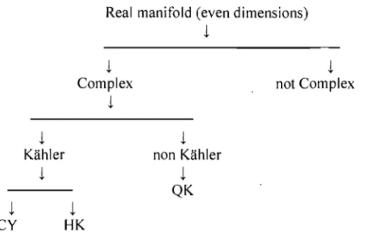
Spin(9) into account. However, it has been proved in [4] that there exists no locally nonsymmetric Riemannian space with this holonomy group. The figure below summarizes the links between the manifolds we will use.

l

Kahler

l

l

l

Real manifold (even dimensions)

l

l

Complex

l

l

non Kahler

l

QK

l

not Complex

CY

HK

FIG. 1.1. Links between manifolds. Notation: Quaternionic Kiih-1er (QK), HyperKiihler (HK), Calabi-Yau (CY).

11

1.2.3. Kahler manifolds

We call 9 a Hermitian metric if gij

=

JikJJgkl' A Hermitian metric 9 on a complex manifold

(M, J)

is called a Kahler me tric if

J

is a constant tensor on

M i.e., if its covariant derivative is equal to zero. Riemannian metrics 9 with

r

ç

U

(m)

are also Kahler metrics. Kahler met ri cs are a natural class of metrics on complex manifolds and generic Kahler metrics on a given complex manifold have

r

=

U(m).

A manifold that admits such a me tric is called a Kahler manifold [3,12].

1.2.4. Calabi-Yau Manifold

Metrics

9

with

r

=

SU(m)

are called Calabi-Yau metrics. Calabi-Yau metrics are locally the same as Ricci-fiat Kahler metrics. Thus, a Calabi-Vau m- fold is a Ricci-fiat Kahler manifold with holonomy

SU(m)

[12]. Some authors also define a Calabi-Yau manifold as a Kahler manifold with vanishing first Chern class [3].

1.2.5. Quaternionic manifold

A Riemannian manifold with holonomy

r

c

Sp(l)

x

Sp(m)

is called a quater-nionic space. These spaces are Einstein if 4m

=

n.

Quaternionic manifolds have non-zero Ricci curvature. If the Ricci curvature is equal to zero, the holonomy groups of these spaces reduces to

Sp(m):

these are the hyperKahler manifolds. Quaternionic Kahler manifolds are manifolds with

r =

Sp(l)

x

Sp(m).

They are in fact not Kahler: they are Einstein, but not Ricci-fiat. They are not locally symmetric spaces. The quaternionic Kahler manifolds we will be working with have negative curvature. Compact, homogeneous, globally symmetric quater-nionic manifolds are called Wolf spaces

[4, HI].

1.2.6. HyperKahler manifold

A Riemannian 4m-manifold

(M, g)

is called hyperKahler if

r

=

Sp(m).

These manifolds are Ricci-fiat, Kahler and thus complex manifolds.

1.2.7. Quaternions

The quaternions are an extension of complex numbers. Quaternions form a

4-dimensional associative algebra denoted by

]HI

=

(1, il, i

2 , i

3)

f"V

JR4

where objects

take the form

q

_{(a+bi l +ci}

2

+di

3 ,

a, b,

c,

dE

JR).

Addition is given by

ql +q2

=

q3

with

q3

(al +a2)+(b

1

+b

2

)i

l

+(CI +c2)i2+(d

1

+d2

)i3 .

Multiplication respects:

1.2.8. Maps

There exists two maps connecting certain manifolds together, namely the

r-map, which links real manifolds to Kahler ones, and the c-r-map, which connects

Kahler manifolds to quaternionic Kahler manifolds:

where

n

1,

n and n

+

1 denote the

complex and quaternionic dimensions

of the real, Kahler and quaternionic spaces respectively

[17].

Important physical

results regarding the c-maps can be found in

[16].

1.3.

PREVIOUS CLASSIFICATIONS

Several classifications of real, Kahler and quaternionic Kahler manifolds were

made over the years using either mathematical or physical approaches. In the

next section, we will introduce the concept used by Alekseevskii to generate the

first classification of these manifolds. We will then expose his results. This will

allow us to better understand the results that we should recover through our

classification.

1.3.1. Isometry Group

A map between two manifolds is called a homeomorphism if it is

continu-ous and has an inverse which is also continucontinu-ous. To illustrate this, suppose we

have two manifolds made of ideal rubber that we can deform at our will. These

manifolds are homeomorphic to each other if we can deform one into the other

13

continuously, that is, without tearing it apart and pasting it.

If

a homeomor-phism and its inverse are differentiable the function is called a diffeomorhomeomor-phism and the two manifolds are said to be diffeomorphic. Two diffeomorphic spaces are regarded as the same space. A diffeomorphism is an isometry if it preserves the metric

[14].

An isometry group of a manifold is the set of all isometries from the manifold onto itself, with the function composition as group operation. Its iden-tity element is the ideniden-tity function. As we will see in the next chapter, isometry groups were used to create the first classification of quaternionic manifolds.

1.3.2. Alekseevskii's classification

Alekseevskii made the first classification of homogeneous quaternionic spaces. He conjectured that all homogeneous quaternionic spaces were exhausted by com-pact symmetric quaternionic spaces and non-comcom-pact normal quaternionic space. Normal quaternionic spaces are quaternionic spaces which admit completely solv-able transitive groups of motions

I.

The rank of the group l that is, the dimension of its Cartan subgroup, is called the rank

R

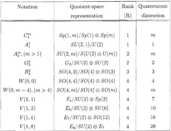
of the normal quaternionic manifold. Alekseevskii classified in

[18]

normal quaternionic manifolds. He found that the rank of these spaces does not exceed four and all spaces of rank sm aller than four are symmetric. He also found that there exists two series of non symmetric quaternionic spaces of rank four which were denoted l;V(p, q) and V(p, q) with p, q integers. Among these, there exists symmetric exceptions:

W(p, q)

with

p

= 0 and

V(p, q)

when

p

=

1. See the table on the next page for Alekseevskii's classi-fication of normal non-compact symmetric quaternionic spaces.

Notation

Quotient-space

1 Rank Quaternionic

representation

(R)

dimension

cm

_l 5p{1, m)/ 5p(1) ® 5p(m) 1

m

Al

1 5U(2,1)/U(2) 1

1

A;'\

(m

>

1) 5U(2, m)/ 5(U(2) U(m))

2

m

G~ G2/5U(2) 5U(2)

2

2

B

3 3

50{ 4,3)/ 50( 4)

®

50(3)

3

3

~V(O,

0)

50(4,4)/50(4)

50(4)

4

4

W(O,m

4),

(m

>

4)

50{4,m)/50(4) 50(m)

4

m

V(l,l)

_F4

/5U(2)

G 5p(3)

4

7 V(1,2) E6/5U(2) G 5U(6)

4

10

V(1,4) E7/SU(2)

50(12)

4

16

V(1,8) Es/5U(2)

4

28

Chapter 2

PHYSICAL DESCRIPTIONS

One can better understand the relevance of studying real, Kahler and quaternionic

Kahler manifolds if we analyze these spaces in the framework of supergravity.

In

this section, we will first of all introduce briefiy the concepts of supersymmetry

and supergravity. We will then explain how our manifolds can be thought of in

this language. This will allow us to better understand another very important

classification of these manifolds that was made a few years ago.

2.1.

SUPERSYMMETRY AND SUPERGRAVITY

Supersymmetry is a continuous symmetry that mixes up fermions (matter)

with bosons (the carriers of force), either in fiat space (supersymmetry) or in

curved space-time (supergravity). A model which possesses local (gauged)

su-persymmetry is called supergravity. A supersymmetric theory cornes with an

algebra which indicates how the various symmetry transformations affects each

other. The possible systems on which the supersymmetry transformations act are

multiplets of particles or quantum fields involving bosons and fermions.

Super-symmetry transformations are generated by quantum operators Q which

trans-form different members of a multiplet into each other i.e., change fermionic states

into bosonic states and vice versa. These operators are in fact spinor operators,

and in four space-time dimensions have at least four real components. Often

called supercharges, they are denoted

Qai

with

Cl: =

1, ... ,4 and

i =

1, ... , N

where

Cl:

is the spinor index and

i

is an internaI index which indicates how many

supersymmetry there is. The simplest supersymmetric theory is called

N

=

1 su-persymmetry. It is invariant under the transformations generated by just the four independent components of a single spinor operator. In the case of additional su-persymmetry, there will be several spinor generators with four components each: these theories are called N-extended supersymmetries. For a flat-space renormal-isable field theory, the allowed values of

N

are 1, 2, and 4.

N

=

3 has the same algebra than

N

=

4.

N

can equal 8 for supergravity theories [27, 28, 29]. In this note, we will be concerned with

N

=

2 supersymmetry in four dimensions. As it is described in details in Section 2.2 of [24], this theory has severalgeneric multiplets. We will be concerned with two of them: the first one being the vector multiplet that contains a (massless gauge) vector field

AM'

two real scalar fields (or one complex scalar field) and two fermions aIl in the adjoint representations of the gauge groups. The second multiplet will be the hypermultiplet, which has four real scalar fields (or two corn plex on es ) and two fermions

[30

J.

2.2.

MODULI SPACE, TARGET SPACE, AND SIGMA MODELS

The set of zero-mode solutions of any quantum field theory fonns a moduli space. Moduli are the parameters labeling a space of degenerate and, usually, physically inequivalent vacua in quantum field theory. The moduli space is the space of geometries or vacua, whose coordinat es are the moduli

[48].

Thus, a moduli space can also be thought of as the space spanned by the scalar fields of a multiplet. A sigma model is a model whose Lagrangian is given by 0MxiO//xj hM// 9ij

where Xi, xj are the coordinates of the target space (the space-time), 9ij is the

metric on the target space, and hM// is the metric of the sigma model. The sigma model metric is the metric appearing in the string world-sheet action. Aiso known as the string metric, this differs from the Einstein metric be a dilaton-dependent Weyl transformation

[48].

A target space is the space-time as se en from the sigma model point of view: it is the moduli space of the sigma model. The target space is the space in which a function takes its values. This is usually applied to the nonlinear sigma model on the string world-sheet, where the target space is

17

itself the spacetime. Recall that the world-sheet is the two-dimensional surface

in spacetime swept out by the motion of a string [48J.

2.2.1. Manifolds' description in supergravity theories.

We can now better appreciate the l'ole of real, Kiihler and quaternionic Kiihler

manifolds

in

physics.

In

N

=

2 supersymmetry, a real manifold is a moduli space

parametrised by the scalar fields in the vector multiplets for five dimensional

su-pergravity. Dimensionally reducing this to four dimensions yields a Kiihler moduli

space for the vector multiplets and further dimension al reduction to three

dimen-sions yields a quaternionic Kiihler manifold which is a moduli space spanned by

the scalar fields of the hypermultiplets. This last fact is used in Section 2.2 of

[24]

to show in detail how a quaternionic

model appears in string theory

by compactifying Type II strings on a Calabi-Yau three-fold.

The physics literature denotes the spaces mentioned above as special manifolds

[25].

Special Kiihler manifolds are those in the

of an T'-map whereas special

quaternionic manifolds are in the image of a c-map. As we will see in the next

subsection, these spaces are generated by certain functions. Although we will

now drop the term special, these are the manifolds we will be concerned with for

the l'est of this note.

2.3.

PREVIOUS CLASSIFICATIONS

In

this section, we introduce in details the notion of. generating functions.

This is done for two reasons. First of aU, generating functions combined with

supergravity are the pillars on which De vVit and Van Proeyen's classification

relies. Secondly, we studied the generating functions in some details in [24] and

will come back to them in later chapters.

2.3.1. Generating functions

The structure of Kiihler manifolds is encoded in a

holomorphie and

h01110geneous function

F(XI)

of degree two

[191.

Unde!' (an inverse) T'-map, these

These cubic functions were classified by De Wit and Van Proeyen in

[25]

where

they were parametrized by:

(2.3.1)

where

dABC

is a syrpmetric tensor and

hK, K

=

A, E, C

represent scalar fields

with certain restrictions.

It

was shown in

[21]

that the

F

functions could be

written in the form

(2.3.2)

where

Xl, l

=1, ... ,

n

+

1 are complex scalar fields corresponding to certain

N

=

2 vector multiplets. As discussed in

[22],

these

F

functions give us important

physical informations such as the Kahler potential

K(X,

X)

and metric

ds

2

_{of a}

Kahler manifold:

- . -1 1 - 2 l - J .

-K(X, X)

=

z(X FI - X FI), ds

=

NIJdX dX , NIJ

=

z(FIJ - FIJ ) (2.3.3)

where

FI

=

8F/8X I.

These

F

functions are referred to as prepotential functions

in the physics literature and determine the Kahler spaces associated to certain

quaternionic spaces. By using the c-map, one can find out the metric of the

associated quaternionic space.

2.3.2. Cecotti's classification

Cecotti classified in

[20]

normal homogeneous Kahler spaces. The

classifica-tion of symmetric Kahler manifolds was already solved sorne time ago by Cremmer

and Van Proeyen

[26].

Cecotti's main result was that there exists two infinite

families of homogeneous non-symmetric Kahler manifolds allowed in

N

=

2

su-pergravity:

K(p, q),

and

H(p, q)

with sorne symmetric exceptions. These spaces

have rank 3 and are in one-to-one correspondence with the homogeneous

quater-nionic spaces found by Alekseevskii

[18].

See the table at the end of this section

for a complete list of the symmetric cases.

2.3.3. De Wit and Van Proeyen's classification

Alekseevskii and Cecotti's classifications of homogeneous spaces was

com-pleted a few years ago by De Wit and Van Proeyen in

[25]

where they used

19

N

=

2 supergravity arguments. They derived a classification of aIl homogeneous quaternionic spaces that were in the image of

cor

map. Their analysis was per-formed completely at the level of special real spaces and amounted to classifying aIl the cubic polynomials

C(h)

generating these spaces. As a result, they found, in addition to the previously classified spaces, a new class of rank-3 spaces of quaternionic dimension larger than 3 and specified in more details sorne of Alek-seevskii's rank-4 spaces. The table at the end of the section shows the complete classification as it is accepted today. Note that the star symbol corresponds to spaces first discussed by De Wit and Van Proeyen1 and that SC stands for pure

N

=

2 supergravity theory in five, four and three dimensions for real, Kahler and quaternionic spaces respectively. This table, which is a summary of the re-sults presented in

[25, 17],

describes aU the homogeneous real, quaternionic and Kahler spaces known before our classification.

C(h)

real

Kahler

quaternionic

1

R

1

sc

U Sp(2n+2,2) U Sp(2n+2)0SU(2)

SC

_U(1)0U(2) U(1,2) U(n,l) U(n+l,2) U(n)0U(1) U(n+l)0U(2)

SC

SU(l,l) G2 (+2)

----uw

SU(2)0SU(2)

L(-I,O)

80(1,1)

[ SU(l,l) ] 3 SO(3,4)

U(l) (SU(2))3

L( -1,

P)

SO(P+l,l) _SO(P+1)

_*

_*

L(O,O)

[80(1,1)]2

[ SU(l,l) ] 3 SO(4,4)

U(l) SO(4)0S0(4)

L(O,

P)

SO(P+1,1)

080(1 1)

SU(l,l) SO(P+2,2) SO(P+4,4) SO(P+l) ,

----uw

0

SO(P+2)0S0(2) SO(P+4)0S0(4)

L(O,

P, p)

Y(P,p)

K(P, p)

W(P,p)

L(q,

P)

X(P,

q)

H(P,

q)

V(P,

q)

L(4m,

P, p)

_*

_*

_*

L(I,I)

SI(3,lR) Sp(6) F1

SO(3) U(3) USp(6)0SU(2)

L(2,1)

SI(3,1C) SU(3,3) E6

SU(3) SU(3)0SU(3)0U(1) SU(6)0SU(2)

L( 4,1)

SU·(6) SO· (12) E7

Sp(3) SU(6)0U(1) SO(12)0SU(2)

L(8,1)

§.fl. E7 Es

F4 E60U(1) E70SU(2)

..

TAB.

2.1. Homogeneous specIal real, Kahler, and quatermomc

spaces. Rank (R) of quaternionic spaces indicated. The rank of

the corresponding real and Kahler spaces is found by decreasing R

by 2 or 1 respectively. Integers

P,

P,

q

and m can take values

2:

1.

0

1

1

2 2

3

3

4

4

4

4

4

4

4

4

4

Chapter

3

OUR CLASSIFICATION

We are now ready to discuss the classification method presented in our paper.

In

[24],

we tried to understand the classification of non-compact symmetric

quater-nionic Kahler manifolds using a different technique than what has been done

previously. More precisely, our classification does not rely on isometry groups

nor on supergravity. Instead, we describe the whole system via

SU(2)

gauge

the-ories with global symmetries

ç;

and exploit the resemblance of this theory with a

sect or of

N

=

2 Seiberg-Witten theOl'y to classify all quaternionic manifolds. We

st art this section by introducing sorne preliminary concepts. We then walk the

reacler through the different steps of our paper, leaving aside the heavy details

and focusing on the premises.

3.1.

PRELIMINARY NOTIONS

3.1.1. Gauge theory

A lagrangian invariant under a continuous symmetry of a certain group G

is said to be globally gauge-invariant if the transformation does not depend on

space-time coordinates. More precisely, a transformation

cPi(X)

- t

UijcPj(x)

which

acts on scalar fields and which leaves a particular lagrangian invariant is called

a global symmetry transformation. The symmetry group

_Uij

E G is independent

of the space-time label

x and is called a gauge group. A lagrangian invariant

uncler a transformation

cPi(X)

- t

Uij(x)cPj(x)

where the gauge group depends on

space-time coordinat es is said to be locally gauge-invariant [27].

In the rest of this note, we will be concerned with an

SU(2)

gauge theory with

global symmetry

Q

where

Q

=

{Sp(n+

1),

G

2 ,

F4' E6, E7, Es}.

In other words, we

will have a lagrangian locally symmetric un der

SU(2)

and globally symmetric

1

under the group

Q.

3.1.2. Seiberg-Witten theory

In 1994, Seiberg and Witten studied the vacuum structure of

N

=

2

super-symmetric gauge theory in four dimensions with gauge group

SU(2).

The theory

is remarkably rich and has physical properties which can be described precisely;

exact formulas can be obtained, for instance, for the metric on the moduli space

of the vacua. This theory allows one to ob tain information about the strong

coupling behavior of

N

=

2 theories in the case of

SU(2)

gauge theory without

matter multiplets [30] and with matter multiplets [38], Global properties of these

theories are contained in what are known as Seiberg-Witten curves [39, 40]. The

model we study in [24] is a sector of this larger framework.

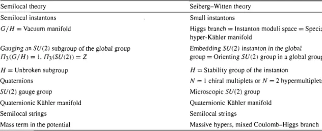
A table of precise connections between elements of the full Seiberg-Witten

theor'y and our theory is provided in Section 3.1 of [24], Our theory being a

small sub-sector of the full theor'y, the complicacies of the original Seiberg-Witten

theory do not affect our analysis. We will come back to this in later subsections.

3.1.3. Instantons

The term instanton has come to refer to localised finite-action solutions of

the classical Euclidean field equations of a theory. In particular, they are

finite-action solutions of the Euclidean

SU(2)

Yang-Mills gauge theory, Instantons

are by definition gauge field configurations. They are associated to self-dual or

anti-dual field strength and carry non-vanishing topological quantum number

[2]. Instantons also play an important role in quantum theOl'y where they lead

IThere is a subtlety here since there might not be a lagrangian description of our model for high global symmetry such as En and F4 . This is discussed in detail in [24].

23 to vacuum tunneling and related phenomena [37]. In our paper, we will be using Euclidean

SU(2)

Yang-Mills instantons in the framework of gauge theory. Although a lagrangian description of our model might not be possible for high global symmetries, this does not affect the existence of these instantons since we find alternative ways to construct them such as embedding the system in F-theory. These details are presented in Section 3.1 of [24].

3.2.

ANALYSIS OF INSTANTONS

The key point we will be using to classify non-compact symmetric quaternionic Kahler manifolds is the following: we look for

SU(2)

gauge theories with global symmetry

9

and find what are called semilocal constrained instantons configu-rations. We know that the low momentum dynamics of these theories are sigma models with quaternionic target spaces.

Thus, our goal is to study instantons in (0.0.1). The analysis of instanton in this theory can be done two ways, both of which will be discussed here and lead to the same results. First, observe that a theory like (0.0.1) will not allow any non-trivial instantons if

(3.2.1) where 7r3 is the third homotopy,

9

is the global symmetry of our theory, and

H

is an ungauged subgroup of

g.

We call the coset space (~) the vacuum manifold

Ml.

A certain type of instantons called constrained instantons will be possible when a subgroup of gis gauged. We will describe this in detail in the next section.

The second way one can analyze instantons in (0.0.1) is through Seiberg-Witten theory. Indeed, when one adds a few terms to (0.0.1) and rewrites the equation in complex coordinates (see Section 3 of [24]), the theory describes a sector called the Higgs branch of the full Seiberg-Witten theory. The vac-uum manifold

Ml

becomes the moduli space of one-instanton. These instantons are described by embedding the

SU(2)

group inside the global symmetry group. The different

SU(2)

orientations de scribe the moduli space of the theory. These

SU(2)

orientations form an S3. In this language, the instanton moduli space will be fibered over a quaternionic Kahler space. Thus, from a mathematical point of view, we have an

SU(2)

instanton fibered over a base space (~). The target space is (~) x

SU(2).

Now that we have laid down the elementary criteria to construct quaternionic manifolds with global symmetry

ç

from instantons configurations, there are sorne important points to analyze.

First, we have to verify if it is possible to construct a Seiberg-Witten-like theory with this global symmetry

ç.

This will be confirmed by the existence of the corresponding Sei berg-Witten curve for the system. A generic curve has the form:

y2 - x3 - a2 x2k (z)

+

alxyl(z)

+

a3yh(z) - a4xf(z) - a6g(z)

= 0 where

ai

are constants and

k(z), l(z), h(z), f(z)

and

g(z)

are polynomials in

z.

The right choice of k, l, h,

f

and 9 can generate a curve that refiects the global symmetry (see Section 3.1 of [24]).

The next step would be to check the existence of instantons in this full Seiberg-Witten theory with global symmetry

ç.

Note that to get a Seiberg-Witten curve for our model, we had to sum over aIl the instantons contributions. Thus the existence of instantons is verified by construction. In the next section, we will construct explicitly these instantons as weIl as the quaternionic spaces on which they are fibered.

3.3.

CONSTRUCTION OF INSTANTONS AND QUATERNIONIC

MANI-FOLDS

The construction of instantons for our model is subtle. First because based on the global symmetries we are using,

ç

=

{Sp(n

+

1),

G

2 ,

E6, E7, Es,

F

4 },

instan-tons are not allowed i.e.,

7r3(Md

=

1 for aIl cases2

. The only allowed instanton

2H

=

{Sp(n) x SU(2),SU(2) x SU(2),SU(6) x SU(2),SO(12) x SU(2),E7 x SU(2),Sp(3) x

25

configuration in our system is the semilocal instanton obtained by gauging an

SU(2)

part of the global symmetry. The second subtlety cornes from the pres-ence of

V(tr(qt . q))

in the action (0.0.1). Namely, the presence of a mass term in the potential makes all the instantons squeeze to zero size. Instantons with this property are called constrained instantons. They resemble the standard instan-tons at short distances but decay exponentially in the infrared limit. Thus, our semilocal instantons are also constrained instantons.

To construct constrained instantons, all we require is for the maximal sub-algebra of the extended Dynkin diagram of

9

to be expressible as a product of two subalgebras and demand that one of these subalgebra be

sp(l).

Constrained instantons are exactly of the gauged

SU(2)

=

Sp(l)

group.

We move on by giving an example which illustrates how to construct the quaternionic manifold which is associated to these instantons. Take for instance the global symmetry group

9

=

Sp(n

+

1) which is studied in detail in Section 3.1 of [24]. The decomposition of the maximal subalgebra into a sum of subalge-bras leads to

sp(n)

EB

sp(l).

Knowing this decomposition, the quaternionic space associated with the global symmetry group

Sp(n

+

1) is built in the following way:

Sp(n

+

1)

= lHIIPn

Sp(n)

x

Sp(l)

.

(3.3.1)

Therefore, the constrained

SU(2)

instantons are non trivially fibered over the quaternionic base lHIIPn. To conclude the argument, we show in [24] that the

vacuum manifold associated to a global symmetry

Sp( n

+

1) is

Ml

=

Q

=

Sp(n+

1)

;::::j s4n+3

1{

Sp(n)

(3.3.2)

Now recall that any

4n

+

3 sphere is equivalent to a

S3

fibration over a quater-nionic base lHIIPn which confirms the validity of our construction.

A few remarks: in order for the reader to see clearly that our classification of quaternionic manifolds is consistent with that of Alekseevskii and De Wit-Van

Proeyen, we will work with the non-compact version of these manifolds. Thus, the compact version of the quaternionic projective space we found earlier i.e.

Sp(n+I) b Sp(n,l)

Q

. .

'f Id . . l . . Sp(n)xSp(l) ecomes Sp(n)xSp(l)' uatermOlllC malll 0 sare wntten III t Ils way III

previous classifications. As we just saw, our method allows us to construct spaces such as lHl]p>n even though these quaternionic manifolds are not in the image of a

c-map. In Section 4 of [24], we show in detail that aIl quaternionic symmetric spaces can be studied using the technique of constrained semilocal instantons.

3.4.

REALISATION OF THE QUOTIENT SPACE

From the steps described in the previous section, the structure of quotient l Sp(n+ 1) l Id b l N I l . l b f

spaces SUCl as Sp(n)xSp(l) S 10U e C ear. ame y, t le maXIma su group 0

Sp( n

+

1)

expressed in terms of a product of two subgroups such that one of those subgroup is

SU(2)

gives us

Sp( n)

x

SU(2).

What remains to study is the precise embedding of the

SU(2)

group inside

9

=

Sp(n

+

1).

Section 3.2 of our paper presents, as an ex ample , the realisation of the quo-tient space Sp(l)~2SP(1) which has been already given in [41, 42J. For the case of

9

=

G2 , we use the embedding of the exceptional complex Lie group G2

(C)

into the complex orthogonal Lie group SO(7,

C).

This allows us to identify the maximal subalgebra

80(4)

=

81L(2)

EB

81L(2)

in G2 .

3.5.

MAGIC SQUARE

The magic square is a mathematical construction which was first developed by Freudenthal, Rosenfeld and Tits in the mid

20

th century and was introduced in string theory a few years later by Gunaydin, Sierra and Townsend [31, 32J.

The magic square is used to show the relation between division algebras, Jordan algebras, and Lie algebras. It consists of a 4 x 4 square with entries given by elements of Lie algebras. The columns of the magic square are defined by the Jordan algebras whereas the rows are defined by the division algebras. The division algebras are the real (IR), complex

(C),

quaternion (1HI), and the octonion

27

(0). The columns are labeled from left to right by

J3(R), J3(C),

J3(Q),

J3(0)

where

J

3

_(OC)

_{is the algebra of 3 x 3 Hermitian matrices over OC. The magic square}

can be represented as follow:

Al A

2

C

3

F

4

A

2 A~

A5

E6

C

3

D6

E7

P4

E6 E7 E8

TAB. 3.1. MagIc square

where

A,

Ci, Di,

,F4

are the usuaI

s'u(i

+

1),

sp(i), so(2i), E

6,7,8

and

F4

Lie

aI-gebras respectively. Through out this note, we will be concerned with the version

of the square associated to the corresponding Lie groups.

3.5.1. Classification of manifolds from the magic square

To construct quaternionic, Kahler, and real manifolds from the elements of the

magic square, we developed a technique called sequential gauging. This method

consists of gauging various subgroups of a gauge group

g

as we move along the

magic square. We argue in Section 4 of

[24]

that the existence of constrained

instantons indicates that we have to gauge by an

SU(2)

subgroup to construct

quaternionic manifolds whereas Kahler manifolds are buil t by gauging a

U

(1 )

subgroup associated to semilocal strings. As indicated in our paper, reai

mani-folds do not require any gauging.

The magic square turns out to be a very useful tool to classify these manifolds

since we can read off from it the global symmetry groups as well as the gauged

maximal subgroups needed to build the quotient space which defines these

man-ifolds. This construction is analyzed in great details in Section 4 of our paper.

Applying the method of sequential gauging through the entire magic square we

find the following results where columns from right to left represent quaternionic

Kahler, Kahler, and two real manifolds respectively3.

SO(3)

SU*(3)

TAB.3.2,

3.5.2. Beyond the magic square

After having described the complete magic square in terms of constrained

stantons and other semilocal defects, we use the same procedure to study other

coset spaces in string theOl'Y. We analyze, in Section 4.5 of our paper, spaces

generated by

U(p)

local symmetry with

SU(n

+

p)

global symmetry and

SU(2)

local symmetry with

SO(p

q)

global symmetry. With these coset spaces, we

exhaust Alekseevskii and De Wit-Van Proeyen's classifications.

In addition of reproducÎng the classification of existing manifolds with our

new technique, we also describe, in Section 4.5 of our paper, the construction

of a new sequence of Kahler manifolds not realized directly in the magic square.

To construct these manifolds, we built coset spaces out of elements of the magic

square and their unused subgroups. By unused we mean here subgroups that our

technique of sequential gauging did not already use to construct real, Kahler and

quaternionic Kahler manifolds.

new sequencing of the magic square follows

rather straightforwardly from our original prescription. Applying this technique

to the elements of the second column of the magic square we found the following

new set of Kahler manifolds:

This construction has recently appeared also in

[35J,

3Notation: the number in the bracket of the global symmetry group Le. E6( +2) denotes the difference between the number of compact and non-compact generators whereas the

*

symbol represents complex matrices with some constraints (see [23]).

29

3.6. G

ENERATING FUNCTIONS REVIsrrED

In previous sections, we discussed the issue of F-functions that could be used

to determine the metric on the quaternionic Kahler manifolds. In this section, we

complete the analysis by postulating the procedure to determine the F-functions

for the

cases. Manifolds with global symmetry

ç;

=

{F4' E6, E7,

Es} are

referred to as the magic cases because they appear in the magic square.

Cecotti constructed in 120] each F-functions corresponding to the normal

quaternionic spaces that appeared in Alekseevskii's classification. However, his

construction of those functions was not explicitly given for the magic cases and

was written in a parametrization that did not allow the use of (2.3.3). In [23],

the authors wrote down the F-functions corresponding to the magic cases but

again in a parametrization that made the computation of the metric in the

for-mat proposed in (2.3.3) not possible. This is why we decided in

[24J

to start

from the beginning and write down these F-functions explicitly in the canonical

parametrization for the magic cases. This form allows one to compute classical

moduli space metrics and Kahler potentials. Note that a general form of the

F-functions which resembles ours was given in

[17]

but where the authors used

an arbitrary linear redefinition of the complex variables instead of the canonical

parametrization.

We start this construction with the cubic functions

C(h)

dABChAhBhc

asso-ciated to real manifolds. These were classified in

[25J.

Imposing certain conditions

[21, 25J

on the generic form of

C(h),

we find a construction for the holomorphie

function

F(X

I)

for the magic cases. These functions can be expressed in terrns

of complex variables

X [

and gamma matrices which generates certain Clifford

algebras. A classification of Clifford algebras in ter ms of gamma matrices already

exits [36]. To classify the several F-functions, we needed to find the right gamma