Statistical methods for investigating the determinants of growth, exports and employment in China

(1)

HAL Id: dumas-00516270

https://dumas.ccsd.cnrs.fr/dumas-00516270

Submitted on 9 Sep 2010

HAL is a multi-disciplinary open access

archive for the deposit and dissemination of sci-entific research documents, whether they are pub-lished or not. The documents may come from teaching and research institutions in France or abroad, or from public or private research centers.

L’archive ouverte pluridisciplinaire HAL, est destinée au dépôt et à la diffusion de documents scientifiques de niveau recherche, publiés ou non, émanant des établissements d’enseignement et de recherche français ou étrangers, des laboratoires publics ou privés.

Statistical methods for investigating the determinants of

growth, exports and employment in China

Donghong Piao

To cite this version:

Donghong Piao. Statistical methods for investigating the determinants of growth, exports and em-ployment in China. Methodology [stat.ME]. 2010. �dumas-00516270�

(2)

Statistical

Statistical methods

methods

methods for

for

for investigating

investigating

investigating the

the

the determinants

determinants

of

of growth,

growth,

growth, exports

exports

exports and

and

and employment

employment

employment in

in

in China

China

UFR de Mathématique et d'Informatique Master 1 Statistique 2009-2010

(3)

Abstract

This paper examines the effects of employment and exports on China's economic growth. Based on export-augmented Cobb-Douglas production function, a set of panel data is used to estimate the contribution of economic growth from exports and employment. We find that both the impacts of exports and employment are positive in the China's economic growth. Besides, we also analyse these effects in different regions in China. The result reveals that the relationship between exports and GDP in the east coastal region is stronger than that in the other regions; the similar situation happens to employment.

Key Key Key

(4)

Acknowledgement

This paper could not be finished without the help and support of many people who are gratefully acknowledged here.

First of all, I would like to show my deepest gratitude to my supervisor, Professor Bertrand KOEBEL, who has led me to doing a research and offered me valuable ideas, suggestions and criticisms with his profound knowledge and rich research experience.

What's more, I wish to extend my thanks to UFR de Mathématique et d'Informatique. I owe special thanks to my professor, Armelle Guillou, for her help

in the last year.

Thanks are also due to my friends, who never failed to give me great encouragement and suggestions. Special thanks should go to Miss. Li Yuanyuan for her brainstorming with me when I failed coming up with ideas.

At last but not least, I would like to thank my family for their support all the way, I am thankful to all my family members for their thoughtfulness and encouragement.

(5)

Table

Table of

of

of contents

1.

1. 1. Introduction

Introduction

In the ranking of the largest economies of the world measured by the gross domestic products (GDP), China stood at the 15th _{position in 1978, but in 2008 the ranking placed}

it at the 3th _{position and this year it will be at the 2}nd _{position instead of Japan. In the}

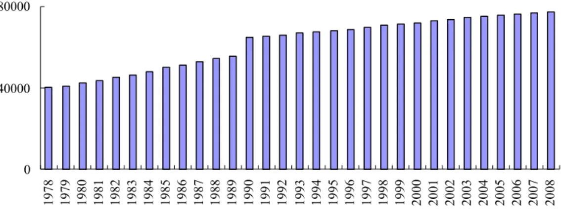
recent 30 years, exports and GDP have increased rapidly (Figure 1) in China. Exports have grown from 164 19 million yuan to 9 936 306 million yuan, while GDP has risen from 364 500 million yuan to 30 285 300 million yuan with an average growth rate over 9%1_{. China has also experienced a process of rapid expansion in employment (Figure 2)}

during this period - 402 million persons were employed in 1978, compared to 775 million persons in 2008, which has played a very important role in China's economic development.

The relationship between foreign trades and economic growth has been investigated in China. Although most of the empirical work supports that the exports led economic growth in China, there is no overall consensus on this issue. Yongjun Li and Justin Yifu Lin (2003) think, according their estimation, a 10% increase in exports will lead to a 1% increase of GDP on average. Shen Lisheng and Wu Zhenyu (2003) gived a method for measuring the contribution to GDP from exports through the I/O table analysis. They found that the rate of contribution from per unit export decreased from 1997 to 2001. Additional, researches based on provincial data have also been carried on these years. Christer Ljungwall (2006) analyzed the relationship between GDP and export at the provincial level, and he found that the export-led growth (ELG) hypothesis is validated in 13 of the 27 provinces in the sample. He Dong and Zhang Wenlang (2010) using input-output analysis showed that the relationship between GDP and exports is stronger in the more developed coastal areas than in the less developed inland areas.

(7)

0 100000 200000 300000 19 78 19 79 19 80 19 81 19 82 19 83 19 84 19 85 19 86 19 87 19 88 19 89 19 90 19 91 19 92 19 93 19 94 19 95 19 96 19 97 19 98 19 99 20 00 20 01 20 02 20 03 20 04 20 05 20 06 20 07 20 08 GDP Export Figure

FigureFigureFigure 1.1.1.1. GDPGDPGDPGDP andandandand ExportExportExportExport 1978-2008(Unit:1978-2008(Unit:1978-2008(Unit:1978-2008(Unit: 100100100100 millionmillionmillionmillion yuan)yuan)yuan)yuan)

Figure

FigureFigureFigure 2.2.2.2. EmploymentEmploymentEmploymentEmployment 1978-20081978-20081978-20081978-2008 (Unit:(Unit:(Unit:(Unit: 10101010 000000000000 persons)persons)persons)persons)

0 40000 80000 1 9 7 8 1 9 7 9 1 9 8 0 1 9 8 1 1 9 8 2 1 9 8 3 1 9 8 4 1 9 8 5 1 9 8 6 1 9 8 7 1 9 8 8 1 9 8 9 1 9 9 0 1 9 9 1 1 9 9 2 1 9 9 3 1 9 9 4 1 9 9 5 1 9 9 6 1 9 9 7 1 9 9 8 1 9 9 9 2 0 0 0 2 0 0 1 2 0 0 2 2 0 0 3 2 0 0 4 2 0 0 5 2 0 0 6 2 0 0 7 2 0 0 8

Source:Comprehensive Statistical Data and Materials on 60 Years of New China

This paper uses a panel data set of 30 provinces, municipalities and autonomous regions in China from 1978 to 2008 to analyse the determinants of China's economic growth and tries to find the contribution of China's economic growth from employment and exports. Besides using static panel data models, dynamic panel data model is also introduced to

(8)

analyse the effects of exports and employment to economic growth. Furthermore, we examine these effects in different regions.

This paper is divided into 5 parts. Part 1 is the introduction. The next part presents the empirical method, in which we will mainly introduce panel data models and the correspondent estimations. The third part introduces our empirical model and the data we choose. The fourth part is the key part, where we will report and analyse the results of the estimation. And finally summaries and conclusions are provided.

(9)

2.

2. 2. Empirical

Empirical

Empirical method

method

2.1 2.1 2.1

2.1 IntroductionIntroductionIntroductionIntroduction ofofofof ppppanelanelanel daneldddataataataata mmmmodelsodelsodelsodels

In recent years, panel data estimation approaches have become widely used. Panel (or longitudinal) data are both cross-sectional and time-series. There are multiple entities, each of which has repeated measurements at different time periods. Therefore, the variables in panel data models have double subscripts with i denoting individuals and t denoting time. As for our study, a panel data set is used for GDP, capital stock, employment and exports in each province of China from 1978 to 2008.

2.2 2.2 2.2

2.2 StaticStaticStaticStatic ppppanelanelanelanel ddataddataataata mmmmodelsodelsodelsodels

Static panel data models is that independent variables do not include lagged dependent variables. Generally, the panel model is given by:

T 1,..., t ; N 1,..., i ' it it = +Χ + + = = Υ α_it β_it µ_i ε_it (2-1)

whereΥ_it (1×1) is the dependent variable, Χit =(Χit₁,L,Χitk)' (1×k) are dependent

variables, α_it(1×1)and (βit₁,L,βijk)'(1×k) are the parameters to estimate and μi and

it

ε are the unobserved effects. This model is under a set of assumptions:

) , 0 ( ~ : Η1 μ_i IDD σ_μ ) , 0 ( ~ : Η2 ε it IDD σ ε i μ : Η₃ is independent of ε ._it

(10)

1) α_i =α_j,β_i = β_j: Using ordinary least squares (OLS) method will provide unbiased, efficient, and consistent estimations.

2) α_i ≠α_j,β_i = β_j : Including fixed effects and the random effects, estimation using separately the least squares dummy variable model (LSDV), the generalized least squares (GLS) and the feasible generalized least squares (FGLS).

3) α_i ≠α_j,β_i ≠ β_j: This model is more complex.

There are two important regressions: the fixed effects regression and the random effects regression. Fixed effects regression is the model to use when we want to control for omitted variables that differ between cases but are constant over time. It lets us use the changes in the variables over time to estimate the effects of the independent variables on our dependent variable, and is the main technique used for analysis of panel data. Statistically, fixed effects are always a reasonable thing to do with panel data (they always give consistent results) but they may not be the most efficient model to run. Random effects will give you better P-values as they are a more efficient estimator. We can utilize the Hausman test to determine which model to be used.

2. 2. 2.

2.3333 DynamicDynamicDynamicDynamic ppppanelanelanel daneldddataataataata mmmmodelsodelsodelsodels

In many economic issues, the future is often correlated with the past. This is to say that

it

y is related to its past realizations y_it_-₁. The dynamic nature of the model reflects the real relationship between the independent and dependent variables more accurately. Thus, the dynamic panel data model is specified as below.

T 1,..., t ; N 1,..., i ' it 1 -it=αit+γyit +x βit+μi+εit = = y (2-2)

Under a set of assumptions: ) , 0 ( ~ : Η₁ μ_i IDD σ_μ ,

(11)

) , 0 ( ~ : Η₂ ε_it IDD σ_ε . i μ : Η₃ is independent of ε ._it

However, the introduction of the lagged dependent variable can pose a variety of problems. For example, the dependent variables Yit and Yit − 1 are functions of μi , and

estimation using OLS will result in biased, inefficient, and inconsistent estimates. Arellano and Bond(1991) used Generalized method of moments (GMM) to estimate dynamic panel data models.

Taking the first difference of the model and we can get:

1 -1 -it ' it ' 2 -it 1 1 -it it-y = ( -y )+(x -x ) + -y γ y_it β ε_it ε_it (2-3) Then we have: t t t t ε β γ Δ ) ΔΧ ΔΥ ( ΔΥ -1 _⎟⎟+ ⎠ ⎞ ⎜⎜ ⎝ ⎛ = (2-4) where ∆Υ_i =(y_i₁,L,y_iT)', ∆Χ_i =(x_i₁,L,x_iT)', and ∆ε_t =(ε₁,L,ε_iT)'.

We can find y_i₀ is highly correlated with y −_i₁ y_i₀ and is uncorrelated to ε −_i₂ ε_i₁. Assuming that the explanatory variables are strictly exogenous, we can use all of them as additional instruments for estimating the parameters. That is, the instrumental variables matrix Ζ is given by_i ⎟ ⎟ ⎟ ⎟ ⎟ ⎠ ⎞ ⎜ ⎜ ⎜ ⎜ ⎜ ⎝ ⎛ = − , , , ) , , ( 0 0 0 0 0 ) , , , , ( 0 0 0 ) , , , ( ' ' 0 2 1 0 ' ' 0 1 0 ' ' 0 0 iT i iT i i iT i i i iT i i i x x y y y x x y y x x y Z L L L O M L L L L (2-5) It is orthogonal if

(

'∆

)

=0 ΕZ ε_i _i (2-6)

(12)

0 1 ' 1 _∆ ₌

∑

= i N i i n Z ε (2-7)

We can get the criterion function as below:

⎟ ⎠ ⎞ ⎜ ⎝ ⎛ ∆ Φ ⎟ ⎠ ⎞ ⎜ ⎝ ⎛ ∆ =

_∑

= − = N i i i i N i i Z n Z n q 1 ' 1 ^ 1 ' 1 1 ε ε (2-8) Where,

(

)

i N i i i i i i i N i i i N i i Z N Z N Z N Ζ ∆ ∆ Ε = ⎟ ⎠ ⎞ ⎜ ⎝ ⎛ Ζ ∆ ∆ Ε = ⎟ ⎠ ⎞ ⎜ ⎝ ⎛ ∆ = Φ

∑

= = = 1 ' ' ' 1 ' 1 ' 1 1 1 var ε ε ε ε ε (2-9) In fact,

(

_N G

)

i i∆ = Ι ⊗ ∆ Ε ' 2 ) ( ε ε σ_ε (2-10) Where, ⎟ ⎟ ⎟ ⎟ ⎟ ⎠ ⎞ ⎜ ⎜ ⎜ ⎜ ⎜ ⎝ ⎛ − − − − − = 1 2 1 0 0 0 0 0 0 0 1 2 1 0 0 0 0 1 2 L M M M O M M L L G (2-11)

From (2-9) and (2-10) we can get:

i N i i N

∑

ZGZ = = Φ 1 ' 2 1 ε σ (2-12)

Taking the derivative of the criterion function:

(

)

(

)

_⎟⎟ ⎠ ⎞ ⎜ ⎜ ⎝ ⎛ ⎥ ⎦ ⎤ ⎢ ⎣ ⎡ ⎟⎟ ⎠ ⎞ ⎜⎜ ⎝ ⎛ ∆Χ ∆Υ − ∆Υ ⎟ ⎠ ⎞ ⎜ ⎝ ⎛ ⎟ ⎠ ⎞ ⎜ ⎝ ⎛ ∆Χ ∆Υ = ⎟⎟ ⎠ ⎞ ⎜⎜ ⎝ ⎛ ∂ ∂

∑

= − − = = − N i i i i i N N i i i N N i i i i N Z ZGZ Z q 1 1 1 1 1 ' 1 1 ' 1 1 _, _, β γ β γ (2-13)

(13)

Take =0 ⎟⎟ ⎠ ⎞ ⎜⎜ ⎝ ⎛ ∂ ∂ β γ q

, then we can get the estimates using the GMM:

(

)

(

)

(

)

⎭ ⎬ ⎫ ⎟ ⎠ ⎞ ⎜ ⎝ ⎛ Υ ⎟ ⎠ ⎞ ⎜ ⎝ ⎛ ⎩ ⎨ ⎧ ⎟ ⎠ ⎞ ⎜ ⎝ ⎛ ∆Χ ∆Υ − ⎭ ⎬ ⎫ ⎟ ⎠ ⎞ ⎜ ⎝ ⎛ ∆Χ ∆Υ ⎟ ⎠ ⎞ ⎜ ⎝ ⎛ ⎩ ⎨ ⎧ ⎟ ⎠ ⎞ ⎜ ⎝ ⎛ ∆Χ ∆Υ = ⎟⎟ ⎠ ⎞ ⎜⎜ ⎝ ⎛

∑

= − = = − − = − − = = − N i i i N N i i i N N i i i i N N i i i i N N i i i N N i i i i N GMM Z GZ Z Z Z GZ Z Z 1 ' 1 1 1 ' 1 1 ' 1 1 1 1 1 ' 1 1 1 ' 1 1 ' 1 1 , , , β γ (2-14)

When independent variables x_it are predetermined variables, when s<t, Ε(x_itε_it)≠0, when s≥t, Ε(x_itε_it)=0. Therefore, only

(

'

)

1 , ' 0 0, i , , is− i x x y L is instrumental variables of the model (2-3) at the time s. In this situation, the instrumental variables of estimation GMM is as below: ⎟⎟ ⎟ ⎟ ⎟ ⎟ ⎟ ⎠ ⎞ ⎜⎜ ⎜ ⎜ ⎜ ⎜ ⎜ ⎝ ⎛ = − − , , , , ) , , , ( 0 0 0 0 0 0 ) , , , , ( 0 0 0 ) , , ( ' 1 , ' 1 ' 0 2 , 1 0 ' 2 ' 1 ' 0 1 0 ' 1 ' 0 0 T i i i T i i i i i i i i i i i i x x x y y y x x x y y x x y Z L L L M O M M L L L (2-15)

Thus, we can get the estimations using GMM when x_it are predetermined variables according to (2-14) and (2-15).

From (2-5) and (2-15), we can know that there may be too many instrumental variables (IV) in the model, which is not reasonable. Generally, we just use the IV that is useful and adjust the matrix of instruments accordingly.

In addition, Arellano and Bond (1991) also proposed the test for over-identifying restrictions, and the statistic of Sargan is given as below:

(14)

) Δ ( ) Δ ( ) Δ ( Δ ^ ' 1 ' ^ 1 ^ ' ' ^ ε Z Z ε ε Z Z ε m i _i n i i i − = ⎥ ⎦ ⎤ ⎢ ⎣ ⎡ =

_∑

Under the null hypothesis of Sargan test,

) ( ~ χ2 L K

m −

(15)

3.

3. 3. Empirical

Empirical

Empirical mode

mode

modellll &

&

& Data

Data

Data selection

selection

3.1 3.1 3.1

3.1 EmpiricalEmpiricalEmpiricalEmpirical mmmmodelodelodelodel

This approach is based on a Cobb-Douglas production function; that is, output is a function of capital, labor, and a term for total factor productivity. And in order to analyse the contribution of exports we consider the export-augmented Cobb-Douglas production function: γ β α E L K A = Υ (3-1)

where Y denotes the aggregate output; A denotes the efficiency parameter; K denotes the capital stock; L denotes the labor input; and E denotes the exports. Taking logarithmic transformation to linearize (3-1) we have:

E L K A ln ln ln ln lnΥ= +α +β +γ (3-2)2

Therefore, we can get the model as below:

it i it it it it = β +β lnK + β lnL + β lnE +μ +ε Υ ln ₀ ₁ ₂ ₃ (3-3)

where β₀_, β₁, β₂, β₃ are the parameters to be estimated.

LnYitdenotes the natural logarithm of aggregate output in the ithprovince in the tthyear.

LnKitdenotes the natural logarithm of capital stock in the ithprovince in the tthyear.

2 _{Using the neoclassical trade theory (NTT) we will have the same model. NTT will be evaluated in a neoclassical}

production function framework incorporating an additional factor of production (exports) into the production function because the exports must have a positive effect on aggregate output . The augmented neoclassical production function is specified as follows: ) , , ( Υ= f K L E

The econometric specification of this relationship will be captured in various bivariate (aggregate output and exports) models without exogenous variables and various bi-variate models with exogenous variables, all expressed in logarithmic form. Below is a representation of an econometric model of bi-variate form with exogenous variables:

E β L β K β β + ln + ln + ln = Υ ln ₀ ₁ ₂ ₃

(16)

LnLitdenotes the natural logarithm of labor input in the ithprovince in the tthyear.

LnEitdenotes the natural logarithm of exports in the ithprovince in the tthyear.

μidenotes the unobserved effects of the ithprovince.

εit denotes the unobserved effects of the ithprovince in the tthyear.

3.2 3.2 3.2

3.2 DataDataDataData selectionselectionselectionselection

Aggregate Aggregate Aggregate

Aggregate outputoutputoutputoutput

The real GDP of each province of China is used to express aggregate output3 _{and take}

1952 as the base year, which is used throughout this paper.

deflator GDP GDP Nominal GDP Real =

We use this formula as follow to calculate GDP deflator.

[

⎩ ⎨ ⎧ > = = 1952 t , ) 100 / Ι ( * GDP / GDP 1952 t , 1 D 1 -it it it it

Where Dit denotes the GDPdeflator of the ith province in the tth year; GDPit denotes the

nominal GDP deflator of the ith_{province in the t}th _{year; I}

itdenotes the GDP indices of the

ith _{province in the t}th _{year (Data are calculated at constant prices and preceding}

year=100)4_.

Capital Capital Capital Capital stockstockstockstock

Wu (2007) has proposed a method of calculating capital stock for China’s regional economies5 _{and we use this kind of data. The general technique of calculating capital}

stock values is the perpetual inventory approach (PIM):

3 _{Chongqing which is created on 14 March 1997 was part of Sichuan province. Therefore, in this paper we}

amalgamate the data of Chongqing and Sichuan.

4 _{Owing to absence of Hainan's GDP indices, we utilize the average GDP indices of the whole China.}

5 _{Capital stock data are in 1952 constant prices from 1952-2006.Wu(2007) indicate:}_{"Economists specializing in the}

Chinese economy have been puzzled by the discrepancy between national and regional data....One possible explanation is that since the mid 1990s capital has become very mobile in China and a lot of cross-regional investment has taken place. As a result, some investment and hence capital formation have been claimed by both the home and hosting regions."

(17)

t i t i t i K K K, =(1−δ) ,−1+∆ ,

where Ki,t is the value of capital stock for the ith region in the tth year; ΔKit is the real

value of incremental capital stock and δ is the rate of depreciation6_.

Labor Labor Labor Labor inputinputinputinput

Labor input should be measured by the standard labor time and labor intensity, but we cannot gain associated data. Therefore, in this paper we use the number of employment of each province of China to represent labor input7_.

Exports Exports Exports Exports

The real exports of each province of China are used, and we do not consider the trade between any two provinces.

6 _{The rates of depreciation are different for different regions.}

7 _{These data are from}_{Comprehensive Statistical Data and Materials on 60 Years of New China Published by China}

(18)

4.

4. 4. Results

Results

4.1 4.1 4.1

4.1 StaticStaticStaticStatic ppppanelanelanelanel ddddataataataata mmmmodelsodelsodelsodels inininin thethethethe wholewholewholewhole countrycountrycountrycountry

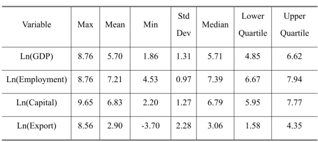
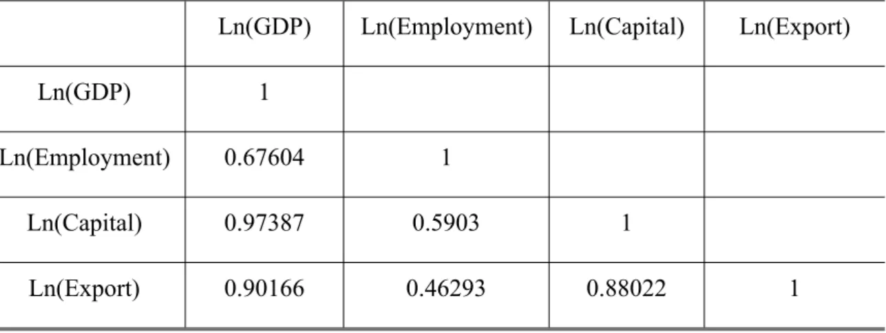
The data used in this study are publicly available from government agencies. The National Bureau of Statistics of China publishes data on nominal GDP and we transform them to real GDP taking 1952 as the base year. The capital stock is calculated in the constant prices in 1952 according to Wu (2007). Table 1 reports the summary of the descriptive statistics on the natural logarithm of GDP, employment, capital stock, exports in the whole country (include 30 provinces) from 1978 to 2008 and Table 2 reports the correlation coefficients of these variables.

Table Table Table

Table 1.1.1.1. TheTheTheThe summarysummarysummarysummary ofofofof thethethethe vvvvariableariableariableariablessss inininin thethethethe wholewholewholewhole countrycountrycountrycountry

Variable Max Mean Min

Std Dev Median Lower Quartile Upper Quartile Ln(GDP) 8.76 5.70 1.86 1.31 5.71 4.85 6.62 Ln(Employment) 8.76 7.21 4.53 0.97 7.39 6.67 7.94 Ln(Capital) 9.65 6.83 2.20 1.27 6.79 5.95 7.77 Ln(Export) 8.56 2.90 -3.70 2.28 3.06 1.58 4.35

(19)

Table 2.2.2.2. CorrelationCorrelationCorrelationCorrelation coefficientcoefficientcoefficientcoefficientssss ofofofof vvvariablevariableariableariablessss inininin thethethethe wholewholewholewhole countrycountrycountrycountry

Ln(GDP) Ln(Employment) Ln(Capital) Ln(Export)

Ln(GDP) 1

Ln(Employment) 0.67604 1

Ln(Capital) 0.97387 0.5903 1

Ln(Export) 0.90166 0.46293 0.88022 1

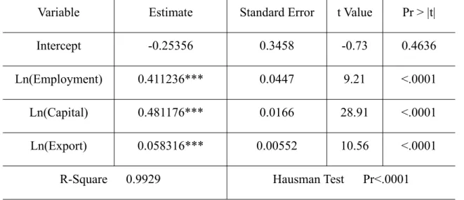
According to Hausman test8 _{(Pr<0.0001), we use fixed estimation method. The results}

are reported in Table 3. As we can see, the estimates of the coefficients of the logarithm capital and labor are significant at 1% level. In this study, we get the estimations for the contributions of capital and labor are 48.1% and 41.1%, respectively. What’s more, the estimate of the coefficient of exports is small (0.0583) but also significant at 1% level, which means that exports has an important impact on GDP. To be specific, GDP increases 0.06% when exports increase 1%. In the whole country, the impacts of employment and exports are both positive for the economic growth. However, the impact of employment is stronger than exports.

As for the positive contributions to GDP of employment and exports, there are several reasons. First, due to the economic reform in China since 1978, a lot of foreign enterprises have entered and invested in China. Therefore, much employment was provided. That is one of the most important reasons for China's economic growth. And in the recent years, China's policy and the huge number of cheap labor (Not only is unskilled labor has low-priced, highly trained labor is also cheap) have attracted a lot of enterprises of original equipment manufacturer (OEM) like Foxconn. That constitutes the inducement of the exports growth. The growth of exports has led to the economic growth,

8 _{The hausman test tests the null hypothesis that the coefficients estimated by the efficient random effects estimator are}

(20)

which in turn attracted more enterprises into China at the same time.

Table

TableTableTable 3.3.3.3. ResultsResultsResultsResults ofof sssstaticofof tatictatictatic ppppanelanelanelanel ddddataataataata mmmmodelsodels inodelsodelsininin wholewholewholewhole countrycountrycountrycountry

***, **, * denote statistically significant at 1%, 5%, and 10% level respectively.

4.2 4.2 4.2

4.2 DynamicDynamicDynamicDynamic ppppanelanelanelanel ddddataataataata mmmmodelsodelsodelsodels inininin thethethethe wholewholewholewhole countrycountrycountrycountry

Static panel data model does not consider dynamic effects of GDP. In fact, lagged values of GDP may have effects on current GDP. Therefore, in this part we apply the dynamic panel data model to consider the influence of the lagged GDP. According to (2-2), we get the empirical model as below:

it i it it it it it = β +γlnΥ − +β lnK +β lnL +β lnE +μ +ε Υ ln ₀ ₁ ₁ ₂ ₃ (3-4)

Since the result of the estimation using OLS is biased, inefficient, and inconsistent estimates, we estimate the coefficient using GMM that Arellano and Bond (1991) proposed for the dynamic panel data model. In the equation (3-4) there is the lag of dependent variable, so we take the first difference of the model and get the empirical model as follows:

Variable Estimate Standard Error t Value Pr > |t|

Intercept -0.25356 0.3458 -0.73 0.4636

Ln(Employment) 0.411236*** 0.0447 9.21 <.0001 Ln(Capital) 0.481176*** 0.0166 28.91 <.0001 Ln(Export) 0.058316*** 0.00552 10.56 <.0001

(21)

it it it it it it γΔlnΥ βΔlnK β ΔlnL β ΔlnE Δε Υ ln Δ = ₋₁+ ₁ + ₂ + ₃ + (3-5)

Estimation by a two-step GMM method is chosen here and five lags of the dependent variables are used as instruments.

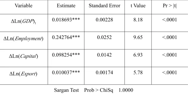
Because the number of instrumental variable (IV) is more than number of endogenous variables, we should use Sargan test to check the over-identifying restrictions. According to Table 4, we can find that Sargan test pass the test at 10% level, so over-identifying restrictions test is valid. Thus, IV is uncorrelated with the error term, which shows that IV is valid9_.

Table 4.4.4.4. ResultsResultsResultsResults ofofofof ddynamicddynamicynamicynamic ppppanelanelanelanel ddataddataataata mmmmodelsodelsodelsodels inin theininthethethe wholewholewholewhole countrycountrycountrycountry

1 ) Ln( Δ GDP 0.018693*** 0.00228 8.18 <.0001 ) Ln( Δ Employment 0.242764*** 0.0252 9.65 <.0001 ) Ln( Δ Capital 0.098254*** 0.0142 6.93 <.0001 ) Ln( Δ Export 0.010037*** 0.00174 5.78 <.0001

Sargan Test Prob > ChiSq 1.0000

***, **, * denote statistically significant at 1%, 5%, and 10% level respectively.

1

)

ln(GDP denotes the one lag of ln(GDP).

Table 4 reports the results of dynamic panel data model in the whole country. We can find that all the estimates are significant at 1% level and all coefficients are positive including

(22)

the estimate of Δln(GDP)₁ , which captures the dynamic relationship in the growth of GDP. For this, we can explain as follows. Firstly, the growth of GDP in the last year will bring more capital input this year; therefore, GDP will grow rapidly. Secondly, the rapid growth of GDP in the last term will attract more investors to come into China. Thirdly, anticipation in economy play an important role, and the situation of the growth of GDP in the last term is the base of the anticipation in this term. Therefore, the rapid growth in the last term leads to the growth in the current term.

The effects of ΔLn(Employment) and ΔLn(Export) are also significant and positive for the growth of GDP. From the results, GDP will increase 0.24% when the employment increases 1%, whereas it grows 0.01% when the exports grow 1%.

4.3 4.3 4.3

4.3 AAAAnalysisnalysisnalysisnalysis ofofofof thethethethe sssstatictatictatictatic mmodelsmmodelsodelsodels inininin threethreethreethree geographicalgeographicalgeographicalgeographical regionregionregionregionssss

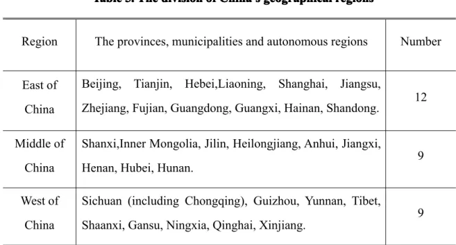
There are the glaring differences of the China's economic development in different regions. The contributions to GDP from employment and exports are different in various regions. In 1978, China transforms its planned economy into a market economy, the east region reformed firstly. Therefore, it develops more rapidly than the other regions. Generally, we divide China into three geographical regions. The detail of the division is reported in Table 5.

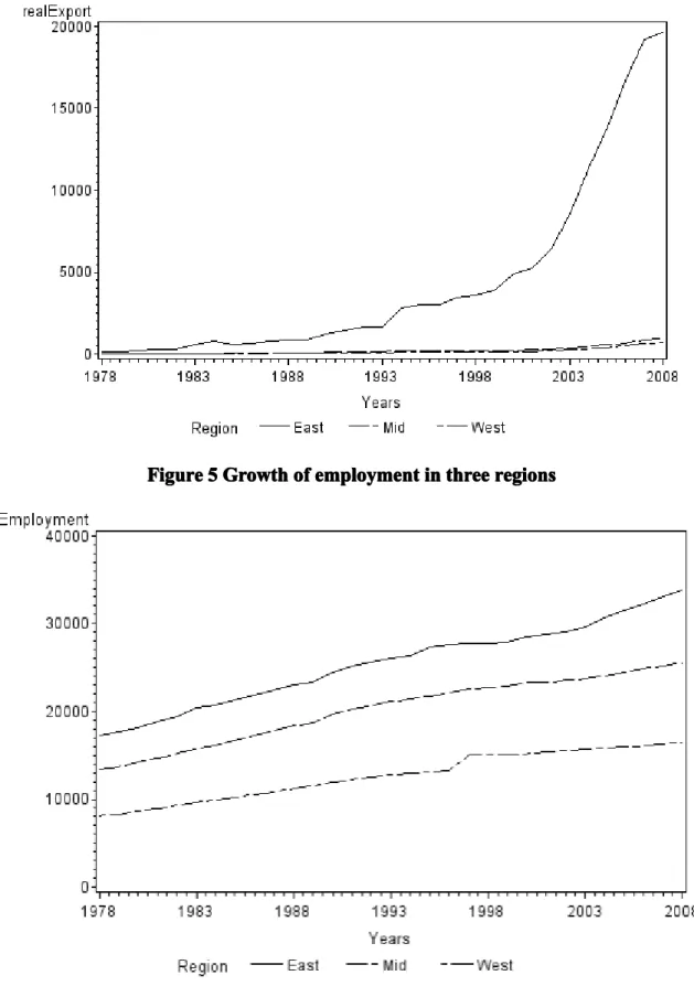
Figure 3 shows the growth of real GDP in different regions. It is obvious that the economy grows faster in the eastern region than the others, and the west region develops slowest. And from Figure 4, real exports of the east region also grow fast, especially in the last decade. Although we can find significant differences in the three regions of China in the respect of both economic growth and exports, Figure 5 indicates that the employment of the three regions grows almost in the same speed. Due to this, it's necessary to analyse the cause of economic growth respectively.

(23)

Table 5.5.5.5. TheTheTheThe divisiondivisiondivisiondivision ofofofof China'sChina'sChina'sChina's geographicalgeographicalgeographicalgeographical rrrregionegionegionegionssss

Region The provinces, municipalities and autonomous regions Number

East of China

Beijing, Tianjin, Hebei,Liaoning, Shanghai, Jiangsu,

Zhejiang, Fujian, Guangdong, Guangxi, Hainan, Shandong. 12

Middle of China

Shanxi,Inner Mongolia, Jilin, Heilongjiang, Anhui, Jiangxi, Henan, Hubei, Hunan.

9

West of China

Sichuan (including Chongqing), Guizhou, Yunnan, Tibet, Shaanxi, Gansu, Ningxia, Qinghai, Xinjiang.

9

Figure Figure Figure

(24)

Figure Figure Figure

Figure 4444 GrowthGrowthGrowthGrowth ofofofof exportexport inexportexportininin threethreethreethree regionsregionsregionsregions

Figure Figure

(25)

In this part, based on the static panel data model we introduce three dummy variables,

w m

e D D

D , , which are specified as follow:

1, The provinces in the eastern region. 0, The provinces in the other regions.

it De _{= ⎨}⎧ ⎩ ⎩ ⎨ ⎧ = . regions other the in provinces The 0, region. middle the in provinces The 1, it Dm

1, The provinces in the western region. 0, The provinces in the other regions. it

Dw _{= ⎨}⎧

⎩

Therefore, the model is represented as below:

it i it it w it it m it it e it it w it it m it it e it it ε μ E Dw β E Dm β E De β L Dw β L Dm β L De β K β β + + × + × + × + × + × + × + + = ) ln ( ) ln ( ) ln ( ) ln ( ) ln ( ) ln ( ln Υ ln 3 3 3 2 2 2 1 0

where e, m, w denote eastern, middle and western region respectively. The variables have the same meaning with (3-3).

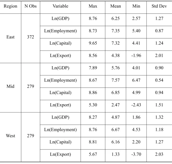
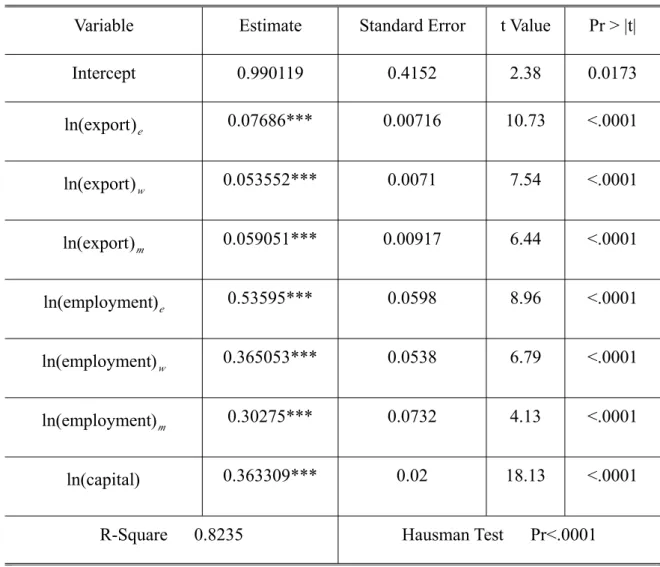
Table 6 reports the summary of the variables in different regions and Table 7 contains the results of the estimation of the coefficients in different regions. We can find all the estimations are significant at 1% level except the intercept. The contribution of GDP from the exports in the eastern area is higher than that in the other two regions, which shows the same result as He Dong and Zhang Wenlang (2010). GDP of the eastern region grows rapidly from 1978, because many foreign direct investments (FDI) were created in many provinces of this region, such as Guangdong, Fujian, Shanghai and so on. That is also why the last global economic crisis brought the greatest impact for the eastern region.

In the western area, although the economic growth is less than the other region, there are a lot of natural resources, such as coal, fossil fuels, rock and mineral resources. Therefore, the contribution of GDP from the exports in the west region achieves almost the level of middle region.

(26)

However, the employment is always the most important factor for the growth of GDP. When the employment increases 1% in the eastern region, GDP will increase 0.54%, whereas in the middle and western regions they are respectively 0.30% and 0.37%.

Table

TableTableTable 6666.... TheTheTheThe summarysummarysummarysummary ofofofof thethethethe vvvvariableariableariableariablessss inininin differentdifferentdifferentdifferent regionsregionsregionsregions

Region N Obs Variable Max Mean Min Std Dev

East 372 Ln(GDP) 8.76 6.25 2.57 1.27 Ln(Employment) 8.73 7.35 5.40 0.87 Ln(Capital) 9.65 7.32 4.41 1.24 Ln(Export) 8.56 4.38 -1.96 2.01 Mid 279 Ln(GDP) 7.89 5.76 4.01 0.90 Ln(Employment) 8.67 7.57 6.47 0.54 Ln(Capital) 8.86 6.85 4.99 0.94 Ln(Export) 5.30 2.47 -2.43 1.51 West 279 Ln(GDP) 8.27 4.87 1.86 1.32 Ln(Employment) 8.76 6.67 4.53 1.18 Ln(Capital) 8.81 6.16 2.20 1.27 Ln(Export) 5.67 1.33 -3.70 2.03

(27)

Table 7777.... ParameterParameterParameterParameter estimatesestimatesestimatesestimates ofofofof staticstaticstaticstatic modelsmodelsmodelsmodels bybybyby regionregionregionregion

Intercept 0.990119 0.4152 2.38 0.0173 e ) export ln( 0.07686*** 0.00716 10.73 <.0001 w ) export ln( 0.053552*** 0.0071 7.54 <.0001 m ) export ln( 0.059051*** 0.00917 6.44 <.0001 e ) employment ln( 0.53595*** 0.0598 8.96 <.0001 w ) employment ln( 0.365053*** 0.0538 6.79 <.0001 m ) employment ln( 0.30275*** 0.0732 4.13 <.0001 ) capital ln( 0.363309*** 0.02 18.13 <.0001

R-Square 0.8235 Hausman Test Pr<.0001

(28)

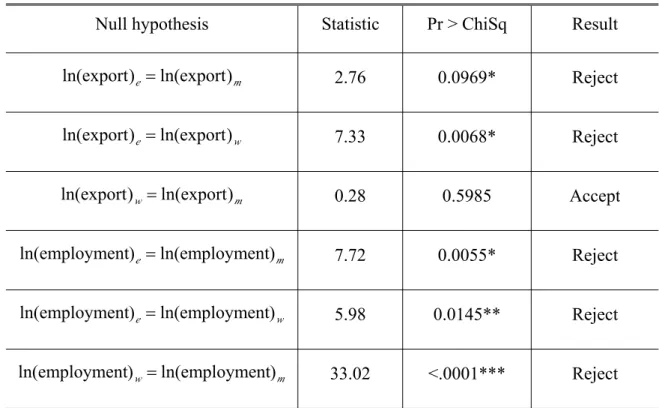
Table 8.8.8.8. WaldWaldWaldWald testtesttesttest ofofofof coefficientcoefficient constraintscoefficientcoefficientconstraintsconstraintsconstraints inininin staticstaticstaticstatic modelsmodelsmodelsmodels

***,**,* denote statistically significant at 1%, 5%, and 10% level respectively.

Table 8 reports the Wald test of coefficient constraints, we cannot accept null hypothesis of Wald test except the hypothesis (ln(export)_w=ln(export)_m). To sum up, we can think that there exist differences of the effect of the exports on GDP among various regions. However, the difference between the effects of the exports on GDP in the western and middle regions is not statistically evident. On the other hand, the contribution of the exports in the east is different from the other two regions and it much higher than the other regions. For employment, there are also the glaring differences in three regions.

4. 4. 4.

4.4444 AAAAnalysisnalysisnalysisnalysis ofofofof thethethethe ddddynamicynamicynamicynamic mmmmodelsodelsodelsodels ininin threeinthreethreethree geographicalgeographicalgeographicalgeographical regionregionregionregionssss

From the dynamic panel data model in the whole country, we find the growth of GDP in the last term is significant and have the positive effect for the growth of GDP. Therefore, we have the reason to believe the dynamic panel data models are more reasonable to

Null hypothesis Statistic Pr > ChiSq Result

m e ln(export) ) export ln( = 2.76 0.0969* Reject w e ln(export) ) export ln( = 7.33 0.0068* Reject m w ln(export) ) export ln( = 0.28 0.5985 Accept m e ln(employment) ) employment ln( = 7.72 0.0055* Reject w e ln(employment) ) employment ln( = 5.98 0.0145** Reject m w ln(employment) ) employment ln( = 33.02 <.0001*** Reject

(29)

analyze the determinants of the China's economic growth. We also build three dummy variables, D_e, D_m, D_w which are specified as follows.

⎩ ⎨ ⎧ = . regions other the in provinces The , 0 region. east the in provinces The , 1 it De ⎩ ⎨ ⎧ = . regions other the in provinces The 0, region. middle the in provinces The 1, it Dm ⎩ ⎨ ⎧ = . regions other the in provinces The 0, region. west the in provinces The 1, it Dw

Therefore, we can get the model as below.

it it it it it it it it it it it it it it it it ε E Dw β E Dm β E De β L Dw β L Dm β L De β K β γ Δ ) ln Δ ( ) ln Δ ( ) ln Δ ( ) ln Δ ( ) ln Δ ( ) ln Δ ( ln Δ Υ ln Δ Υ ln Δ 2 2 2 1 1 1 3 1 + × + × + × + × + × + × + + = ₋

Firstly, we run Sargan test which pass the test at 10% level, so over-identifying restrictions test is valid. We estimate the coefficients by a two step GMM method and five lags of the dependent variables are used as instruments. Table 9 reports the results of parameter estimates using dynamic model. It shows that the coefficients are positive and significant at the level 1%, excluding those of the employment in the western region, exports in the middle and western regions. The same as the static panel data model in the whole country, the growth rate in the last term has the positive effect on the growth in the current term. Compared to the static model, we can find that the relationship between the growth rate of employment and the economic growth rate in eastern region is less strong, which is also true for the relationship between the growth rate of export and GDP.

In addition, table 10 reports the results of Wald test of coefficient constraints in dynamic models, we can find there are differences between the effects of exports in the eastern

(30)

region and in the other regions in the economic growth. Whether in static models or dynamic models, the impact of export in the eastern area is always positive and significant. Therefore, we can say the exports in the eastern area are quit important for its economic growth.

Table Table

TableTable 9999 .... ParameterParameterParameterParameter estimatesestimatesestimatesestimates ofof dynamicofofdynamicdynamicdynamic modelsmodelsmodelsmodels bybybyby regionregionregionregion

1 ) Ln( Δ GDP 0.018998*** 0.00315 6.04 <.0001 ) Ln( Δ Capital 0.090247*** 0.0229 3.93 <.0001 e ) Employment Ln( Δ 0.458069*** 0.1299 3.53 0.0004 m ) Employment Ln( Δ 0.529645*** 0.1604 3.3 0.001 w ) Employment Ln( Δ -0.08571 0.0834 -1.03 0.3046 e ) Ln( Δ Export 0.042723*** 0.0139 3.07 0.0022 m ) Ln( Δ Export -0.01423 0.0128 -1.12 0.265 w ) Ln( Δ Export -0.00735 0.0131 -0.56 0.5737

(31)

Table 10.10.10.10. WaldWaldWaldWald testtesttesttest ofofofof coefficientcoefficient constraintscoefficientcoefficientconstraintsconstraintsconstraints inininin dynamicdynamicdynamicdynamic modelsmodelsmodelsmodels

Considering the negative and insignificant estimates of some coefficients, which does not make sense in the economic context, the results of the dynamic panel data in different regions are not quite satisfying. This might be due to the data we use in this study, which measure the exports without considering the trade between two provinces.

Null hypothesis Statistic Pr > ChiSq Result

m e Δln(export) ) export ln( Δ = 5.35 0.0207** Reject w e Δln(export) ) export ln( Δ = 5.46 0.0195** Reject m w Δln(export) ) export ln( Δ = 0.11 0.7382 Accept m e Δln(employment) ) employment ln( Δ = 0.15 0.695 Accept w e Δln(employment) ) employment ln( Δ = 9.69 0.0019*** Reject w e Δln(employment) ) employment ln( Δ = 0.76 0.3824 Accept

(32)

5.

5. 5. Conclusion

Conclusion

Since the reform (1978) in China, the exports increased more than 600% and they rise at a higher rate than the economic growth rate, the employment almost doubled, increasing from 402 million persons in 1978 to 775 million persons in 2008. According to our estimation, both the exports and the employment are important factors in the China's economic growth. Although the contribution for economic growth from the exports is not so much as that from the employment in the whole country, they both have the positive effects in economic growth. From the dynamic models, we can find the effect of economic growth in the last term is also positive in the economic growth in the current year, which shows the dynamic nature of the economic growth. From 1978, a lot of foreign companies entered the Chinese market and have set up a large number of plants which provided many jobs. Due to the number of the low-priced labor, exports exhibit the evident superiority. Therefore, we can conclude that beside labor and capital, exports also lead to the rapid growth of China’s economy in the past 30 years.

In different regions, we find that there exist the glaring differences in respect of the effects of exports and employment on the economic growth. The economic growth of the east coastal region, which develops more rapidly and is more economically open to the world than the other regions, has a stronger relationship with its exports. Yet in the middle and western regions, the effects of exports do not show evident differences. The impact of employment is also the most important in the eastern region. Although the western area is less developed in China, the increasing of the government's investment promotes the growth of employment, which is the most important factor in the economic growth in the west. Due to the crucial part played by the employment, the fact that a huge number of cheap labors from the middle and west of China go to the east coastal area to find a job may be the one of the most important reasons of the rapid growth of GDP in the eastern region.

(33)

We acknowledge that the specification of the model, the selection of the estimation method and the selection of data will affect the results; therefore, the further improvement is expected.

(34)

References

Alvarez,R. & S,Claro. On the Sources of China’s Export Growth , J(2007), Working Papers Central Bank of Chile,426

ASHFAQUE H. KHAN, Employment Creation Effects of Pakistan's Exports, J(1991),

The Pakistan Development Review,865-877

Bond,S.,A,Hoeffler & J,Temple. GMM Estimation of Empirical Growth Models, (2001),University of Oxford,University of Bristol.

Bosworth,B & S.M.Collins. Accounting for Growth: Comparing China and India, J(2008), Journal of Economic Perspectives, American Economic Association

12943,45-66

Chemeda, EF. The Role of Exports in Economic Growth with Reference To Ethioplan Country, A(2001), Annual Meeting of the Ameriacn Agricultural Economics Association in Chiago.

Dic, Lo. China’s Economic Growth and Labor Employment– Structural Change, Institutional Evolution And Policy Issus.A(2007), Renmin University of China and SOAS, University of London.

He,D. & W,Zhang. How dependent is the Chinese economy on exports and in what sense has its growth been export-led?, J(2010),Journal of Asian Economics 21,87-104

Hu,A. Economic Growth and Employment Growth in China (1978-2001), J.(2004),

Asian Economic Papers, 166-176.

Li,J. A Theoretical Analysis on Measuring the Import and Export Contribution to the Economic Growth, A(2008),The Journal of Quantitative & Technical Economics 200809, 77-86.

Lin,JY. & Y,Li. Export and Economic Growth in China: a Demand-Oriented analysis, J(2003),China Economic Quarterly.

Ljungwall,C. Export-led Growth: Application to China's Provinces, 1978-2001, J(2006),

Journal of Chinese Economic and Business Studies 200604,109-126

Mileva,E. Using Arellano – Bond Dynamic Panel GMM Estimators in Stata, A(2007), Fordham University.

Shen,L. & Z,Wu. The Contribution to Economic Growth from Export in China——Empirical Analysis Based on the I/O Table, j(2003), Economic Research Journal 200311,33-41.

Sinoha-Lopete,R. Export-led growth in southern africa, C(1999), Louisiana State University.

(35)

Vohra, R. Export and Economic Growth: Further Time Series Evidence from Less-Developed Countries, J(2001),International Advances in Economic Research,

345-350.

Wu,Y. A(2007),Capital Stock Estimates for China’s Regional Economies:Results and Analyses,The University of Western Australia.

(36)

Appendix

Appendix A.

A.

A. A. Program

Program

Program SAS

SAS

*Taking nature logarithmic transformation of each variable.

DATA DATA DATA DATA paper.data; set paper.data; lGDP = log(RealGDP); lEmployment = log(Employment); lCapital = log(Capital); lExport = log(RealExport); label lGDP = 'Log(GDP)';

label lEmployment = 'Log(Employment)'; label lCapital = 'Log(Capital Stock)'; label lExport = 'Log(Export)';

RUN RUN RUN RUN;

*The summary of the variables in whole country.

PROC PROC PROC

PROC SUMMARYSUMMARYSUMMARYSUMMARY PRINT max MEAN min STD MEDIAN Q1 Q3 data=paper.data; VAR lGDP lEmployment lCapital lExport;

RUN RUN RUN RUN;

*Correlation coefficient of variables in whole country.

proc proc proc

proc corrcorrcorrcorr data=paper.data;

var lGDP lEmployment lCapital lExport;

run run run run;

*Regression of static panel data models in whole country.

PROC SORTSORTSORTSORT DATA=paper.data; BY code Years; RUN RUN RUN RUN; PROC PROC PROC

PROC panelpanelpanelpanel DATA=paper.data; ID Code Years ;

MODEL lGDP=lEmployment lCapital lExport/fixtwo;

RUN RUN RUN RUN;

*The one and two lag of the variables.

proc panelpanelpanelpanel data=paper.data; ID Code Years;

clag LGDP(1111) LGDP(2222) lEmployment(1111) lCapital(1111) lExport(1111)/ out=GDP_lag;

run run run run;

(37)

*The first difference of the variables and the second difference of log(GDP). DATA DATA DATA DATA GDP_lag; set GDP_lag; detalgdp=LGDP-LGDP_1; detalgdp_1=LGDP_1-LGDP_2; detalEmployment=lEmployment-lEmployment_1; detalCapital=lCapital-lCapital_1; detalExport=lExport-lExport_1;

label detalgdp= 'The first difference of log(GDP)'; label detalgdp_1 = 'The second difference of log(GDP)';

label detalEmployment = 'The first difference of log(Employment)'; label detalCapital = 'The first difference of log(Capital)';

label detalExport = 'The first difference of log(Export)';

RUN RUN RUN RUN;

*Regression of dynamic panel data models in whole country.

proc panelpanelpanelpanel data =GDP_lag; inst depvar;

ID Code Years;

MODEL lGDP=detalgdp_1 detalEmployment detalCapital detalExport/gmm twostep MAXBAND=5555 nolevels noint;

run run run run;

*Set a variable region.

DATA DATA DATA

DATA paper.data; SET paper.data;

if province="Beijing" or province="Tianjin" or province= "Hebei" or province="Liaoning" or province= "Shanghai" or province= "Jiangsu"

or province= "Zhejiang" or province= "Fujian" or province=

"Guangdong"or province="Guangxi"or province="Hainan"or province=

"Shandong"

then Region="East";

else if province="Shanxi" or province="Inner Mongolia" or province=

"Jilin"or province="Heilongjiang"or province="Anhui"or province=

"Jiangxi" or province= "Henan" or province= "Hubei" or province=

"Hunan"

then Region="Mid";

else ifprovince="SichuanChongqing" or province= "Guizhou" or province=

"Yunnan" or province= "Tibet" or province= "Shaanxi" or province=

(38)

"Xinjiang"

then Region="West";

RUN RUN RUN RUN;

*Calculate the sum of the variables in different region and save them.

PROC SUMMARYSUMMARYSUMMARYSUMMARY sum data=paper.data NWAY ; class region years;

VAR realGDP Employment realExport;

OUTPUT OUT=PAPER.SUM SUM=realGDP Employment realExport ;

RUN RUN RUN RUN;

*Drew the three Figures.

PROC gplotgplotgplotgplot data=paper.sum; goption hsize=15cm vsize =11cm;

plot realgdp*years=region/vaxis=0000 to 50000500005000050000 by 10000100001000010000

haxis=1978197819781978 to 2008200820082008 by 5555; symbol interpol=join w=1111;

RUN RUN RUN RUN; PROC PROC PROC

plot Employment*years=region/haxis=1978197819781978 to 2008200820082008 by 5555; symbol interpol=join w=1111;

plot realexport*years=region/vaxis=0000 to 20000200002000020000 by 5000500050005000

haxis=1978197819781978 to 2008200820082008 by 5555; symbol interpol=join w=1111;

RUN RUN RUN RUN;

*The summary of the variables in different regions.

PROC SUMMARYSUMMARYSUMMARYSUMMARY PRINT max MEAN min STD MEDIAN Q1 Q3 data=paper.data; class region;

VAR lGDP lEmployment lCapital lExport;

RUN RUN RUN RUN;

*Set three dummy variables.

DATA DATA DATA

DATA paper.data; SET paper.data;

(39)

province="Liaoning" or province= "Shanghai" or province= "Jiangsu"

or province= "Zhejiang" or province= "Fujian" or province=

"Guangdong"or province="Guangxi"or province="Hainan"or province=

"Shandong");

Middle=(province="Shanxi" or province="Inner Mongolia" or province=

"Jilin"or province="Heilongjiang"or province="Anhui"or province=

"Jiangxi" or province= "Henan" or province= "Hubei" or province=

"Hunan");

West=(province="SichuanChongqing" or province= "Guizhou" or province=

"Yunnan" or province= "Tibet" or province= "Shaanxi" or province=

"Gansu" or province= "Ningxia" or province= "Qinghai" or province=

"Xinjiang");

RUN RUN RUN RUN;

*Regression and WALD test of static panel data models by region.

DATA DATA DATA DATA paper.data; set paper.data; eastlexport = east*lexport; westlexport = west*lexport; middlelexport = middle*lexport; eastlEmployment = east*lEmployment; westlEmployment = west*lEmployment; middlelEmployment = middle*lEmployment;

label eastlexport = 'log(Export) in the east region'; label westlexport = 'log(Export) in the west region'; label middlelexport = 'log(Export) in the middle region'; label eastlexport = 'log(Employment) in the east region'; label westlexport = 'log(Employment) in the west region'; label middlelexport = 'log(Employment) in the middle region';

PROC panelpanelpanelpanel DATA=paper.data; ID Code Years ;

MODEL lGDP=eastlexport westlexport middlelexport eastlEmployment westlEmployment middlelEmployment lCapital/fixtwo;

test eastlexport=middlelexport; test eastlexport=westlexport; test westlexport=middlelexport; test eastlEmployment=middlelEmployment; test eastlEmployment=westlEmployment; test westlEmployment=middlelexport;

(40)

RUN RUN RUN RUN;

*Regression and WALD test of dynamic panel data models by region.

DATA DATA DATA DATA GDP_lag; set GDP_lag; detaeastlGDP_1 = east*detalgdp_1; detawestlGDP_1= west*detalgdp_1; detamiddlelGDP_1 = middle*detalgdp_1; detaeastlexport = east*detalexport; detawestlexport = west*detalexport; detamiddlelexport = middle*detalexport; detaeastlEmployment = east*detalEmployment; detawestlEmployment = west*detalEmployment; detamiddlelEmployment = middle*detalEmployment; label detaeastlGDP_1= 'Deta of east log(GDP)'; label detawestlGDP_1 = 'Deta of west log(GDP)'; label detamiddlelGDP_1 = 'Deta of middle log(GDP)'; label detaeastlexport = 'Deta of east log(Export)'; label detawestlexport = 'Deta of west log(Export)'; label detamiddlelexport = 'Deta of middle log(Export)'; label detaeastlEmployment = 'Deta of east log(Employment)'; label detawestlEmployment = 'Deta of west log(Employment)'; label detamiddlelEmployment = 'Deta of middlel log(Employment)';

RUN RUN RUN RUN; proc proc proc

proc panelpanelpanelpanel data =GDP_lag; inst depvar ;

ID Code Years;

MODEL datalGDP=datalGDP_1 datalCapital detaeastlEmployment detamiddlelEmployment detawestlEmployment detaeastlExport detamiddlelExport detawestlExport

/gmm twostep MAXBAND=5555 nolevels noint; test detaeastlexport=detamiddlelexport; test detaeastlexport=detawestlexport; test detawestlexport=detamiddlelexport; test detaeastlEmployment=detamiddlelEmployment; test detaeastlEmployment=detawestlEmployment; test detawestlEmployment=detamiddlelexport; run run run run;

(41)

Appendix

Appendix B.

B.

B. B. Data

Data

1.

1. 1. GDP

GDP

GDP (100

(100

(100 million

million

million yuan)

yuan)

Codes 1 2 3 4 5 6 7 8 9 10

Years Beijing Tianjin Hebei Shanxi Inner Mongolia

Liaoning Jilin Heilongj iang Shanghai Jiangsu 1978 108.84 82.65 183.06 88 58.04 229.2 81.98 174.78 272.81 249.24 1979 120.11 93 203.22 106.4 64.14 244.96 91.12 187.16 286.43 298.55 1980 139.07 103.52 219.24 108.8 68.4 281 98.59 221.04 311.89 319.8 1981 139.15 107.96 222.54 121.7 77.91 288.61 111.16 228.3 324.76 350.02 1982 154.94 114.1 251.45 139.2 93.22 315.07 121.67 248.42 337.07 390.17 1983 183.13 123.4 283.21 155.1 105.88 364.02 150.14 276.94 351.81 437.65 1984 216.61 147.47 332.22 197.4 128.2 438.17 174.39 318.34 390.85 518.85 1985 257.1 175.7 396.8 219 163.8 518.6 200.4 355 466.8 651.8 1986 284.9 194.7 436.7 235.1 181.6 605.3 227.2 400.8 490.8 744.9 1987 326.8 220 521.9 257.2 212.3 719.1 297.5 454.6 545.5 922.3 1988 410.2 259.6 701.3 316.7 270.8 881 368.7 552 648.3 1208.9 1989 456 283.3 822.8 376.3 292.7 1003.8 391.7 630.6 696.5 1321.9 1990 500.8 311 896.3 429.3 319.3 1062.7 425.3 715.2 756.5 1416.5 1991 598.9 342.8 1072.1 468.5 359.7 1200.1 463.5 824.2 893.8 1601.4 1992 709.1 411.2 1278.5 570.1 421.7 1473 558.1 964 1114.3 2136 1993 863.5 536.1 1690.8 704.7 532.7 2010.8 718 1203.2 1511.6 2998.2 1994 1145.3 732.9 2187.5 826.7 695.1 2461.8 937.7 1604.9 1990.9 4057.4 1995 1507.7 932 2849.5 1076 857.1 2793.4 1137.2 1991.4 2499.4 5155.3 1996 1789.2 1121.9 3453 1292.1 1023.1 3157.7 1346.8 2370.5 2957.6 6004.2 1997 2075.6 1264.6 3953.8 1476 1153.5 3582.5 1464.3 2667.5 3438.8 6680.3 1998 2376 1374.6 4256 1611.1 1262.5 3881.7 1577.1 2774.4 3801.1 7200 1999 2677.6 1501 4514.2 1667.1 1379.3 4171.7 1673 2866.3 4188.7 7697.8 2000 3161 1701.9 5044 1845.7 1539.1 4669.1 1951.5 3151.4 4771.2 8553.7 2001 3710.5 1919.1 5516.8 2029.5 1713.8 5033.1 2120.4 3390.1 5210.1 9456.8 2002 4330.4 2150.8 6018.3 2324.8 1940.9 5458.2 2348.5 3637.2 5741 10606.9 2003 5023.8 2578 6921.3 2855.2 2388.4 6002.5 2662.1 4057.4 6694.2 12442.9 2004 6060.3 3111 8477.6 3571.4 3041.1 6672 3122 4750.6 8072.8 15003.6 2005 6886.3 3697.6 10096.1 4179.5 3895.6 8009 3620.3 5511.5 9154.2 18305.7 2006 7870.3 4359.2 11660.4 4752.5 4791.5 9251.2 4275.1 6188.9 10366.4 21645.1 2007 9353.3 5050.4 13709.5 5733.4 6091.1 11023.5 5284.7 7065 12188.9 25741.2 2008 10488 6354.4 16188.6 6938.7 7761.8 13461.6 6424.1 8310 13698.2 30312.6

(42)

Continue

Codes 11 12 13 14 15 16 17 18 19 20

Years Zhejiang Anhui Fujian Jiangxi Shandong Henan Hubei Hunan

Guang dong Guang xi 1978 123.72 113.96 66.37 87 225.45 162.92 151 146.99 185.85 75.85 1979 157.64 127.31 74.11 104.15 251.6 190.09 188.46 178.01 209.34 84.59 1980 179.68 140.88 87.06 111.15 292.13 229.16 199.38 191.72 249.65 97.33 1981 204.45 170.51 105.62 121.26 346.57 249.69 219.75 209.68 290.36 113.46 1982 233.41 187.02 117.81 133.96 395.38 263.3 241.55 232.52 339.92 129.15 1983 256.23 215.68 127.76 144.13 459.83 327.95 262.58 257.43 368.75 134.6 1984 322.07 265.74 157.06 169.11 581.56 370.04 328.22 287.29 458.74 150.27 1985 427.5 331.2 200.5 207.9 680.5 451.7 396.3 350 577.4 181 1986 500.1 382.8 222.5 230.8 742.1 502.9 442 397.7 667.5 205.5 1987 603.7 442.4 279.2 262.9 892.3 609.6 517.8 469.4 846.7 241.6 1988 765.8 546.9 383.2 325.8 1117.7 749.1 626.5 584.1 1155.4 313.3 1989 843.7 616.3 458.4 376.5 1293.9 850.7 717.1 640.8 1381.4 383.4 1990 898 658 523.3 419.5 1511.2 934.7 824.4 744.4 1471.8 449.1 1991 1081.8 663.6 622 465.1 1810.5 1045.7 913.4 833.3 1780.6 518.6 1992 1365.1 801.2 787.7 559.5 2196.5 1279.8 1088.4 997.7 2293.5 646.6 1993 1909.5 1069.8 1133.5 701.9 2779.5 1662.8 1424.4 1278.3 3225.3 893.6 1994 2689.3 1320.4 1644.4 948.2 3844.5 2216.8 1700.9 1650 4619 1198.3 1995 3557.6 1810.7 2094.9 1169.7 4953.4 2988.4 2109.4 2132.1 5933.1 1497.6 1996 4188.5 2093.3 2484.3 1409.7 5883.8 3634.7 2499.8 2540.1 6835 1697.9 1997 4686.1 2347.3 2870.9 1605.8 6537.1 4041.1 2856.5 2849.3 7774.5 1817.3 1998 5052.6 2543 3159.9 1719.9 7021.4 4308.2 3114 3025.5 8530.9 1911.3 1999 5443.9 2712.3 3414.2 1853.7 7493.8 4517.9 3229.3 3214.5 9250.7 1971.4 2000 6141 2902.1 3764.5 2003.1 8337.5 5053 3545.4 3551.5 10741.3 2080 2001 6898.3 3246.7 4072.9 2175.7 9195 5533 3880.5 3831.9 12039.3 2279.3 2002 8003.7 3519.7 4467.6 2450.5 10275.5 6035.5 4212.8 4151.5 13502.4 2523.7 2003 9705 3923.1 4983.7 2807.4 12078.2 6867.7 4757.5 4660 15844.6 2821.1 2004 11648.7 4759.3 5763.4 3456.7 15021.8 8553.8 5633.2 5641.9 18864.6 3433.5 2005 13437.9 5375.1 6568.9 4056.8 18516.9 10587.4 6520.1 6511.3 22366.5 4075.8 2006 15742.5 6148.7 7614.6 4670.5 22077.4 12496 7581.3 7568.9 26204.5 4828.5 2007 18780.4 7364.2 9249.1 5500.3 25965.9 15012.5 9230.7 9200 31084.4 5955.7 2008 21486.9 8874.2 10823.1 6480.3 31072.1 18407.8 11330.4 11156.6 35696.5 7171.6

(43)

Continue Codes 21 22 23 24 25 26 27 28 29 30 Years Hainan Sichuan &Chong qing

Guizhou Yunnan Tibet Shaanxi Gansu Qinghai Ningxia Xinjiang

1978 16.4 184.61 46.62 69.05 6.65 81.07 64.73 15.54 13 39.07 1979 17.45 205.76 55.28 76.83 7.3 94.52 67.51 15.19 14.36 45.63 1980 19.33 229.31 60.26 84.27 8.67 94.91 73.9 17.79 15.96 53.24 1981 22.23 242.32 67.89 94.13 10.4 102.09 70.89 17.49 17.42 59.41 1982 28.86 275.23 79.39 110.12 10.21 111.95 76.88 19.95 18.22 65.24 1983 31.12 311 87.38 120.07 10.29 123.39 91.5 22.45 20.79 78.55 1984 37.18 358.06 108.27 139.58 13.68 149.35 103.17 26.42 24.78 89.75 1985 43.3 421.2 123.9 165 17.8 180.9 123.4 33 30.3 112.2 1986 48 458.2 139.6 182.3 16.9 208.3 140.7 38.4 34.5 129 1987 57.3 530.9 165.5 229 17.7 245 159.5 43.4 39.6 148.5 1988 77.1 659.7 211.8 301.1 20.3 314.5 191.8 55 50.3 192.7 1989 91.4 745 235.8 363.1 21.9 358.4 216.8 60.4 59.2 217.4 1990 102.5 1186.2 260.1 451.7 24.5 404.3 242.8 69.9 64.8 274 1991 120.5 1383 295.9 517.4 30.5 466.8 271.4 75.1 71.8 335.9 1992 181.7 1624.5 339.9 618.7 33.3 538.4 317.8 87.5 83.1 402.3 1993 258.1 2096.5 416.1 779.2 37.3 661.4 372.2 109.6 103.8 505.6 1994 332 2757.4 524.5 983.8 46 839 453.6 138.4 136.3 662.3 1995 363.3 3459.5 636.2 1222.2 56.1 1036.9 557.8 167.8 175.2 814.9 1996 389.7 4059.2 723.2 1517.7 65 1215.8 722.5 184.2 202.9 900.9 1997 411.2 4601.7 805.8 1676.2 77.2 1363.6 793.6 202.8 224.6 1039.9 1998 442.1 4914.7 858.4 1831.3 91.5 1458.4 887.7 220.9 245.4 1107 1999 476.7 5141.1 937.5 1899.8 106 1592.6 956.3 239.4 264.6 1163.2 2000 526.8 5531.4 1029.9 2011.2 117.8 1804 1052.9 263.7 295 1363.6 2001 558.4 6059.2 1133.3 2138.3 139.2 2010.6 1125.4 300.1 337.4 1491.6 2002 622 6715 1243.4 2312.8 166.6 2253.4 1232 340.7 377.2 1612.7 2003 693.2 7605.9 1426.3 2556 189.1 2587.7 1399.8 390.2 445.4 1886.4 2004 798.9 9072.4 1677.8 3081.9 220.3 3175.6 1688.5 466.1 537.2 2209.1 2005 894.6 10455.6 1979.1 3472.9 251.2 3675.7 1934 543.3 606.1 2604.2 2006 1052.9 12129.4 2282 4006.7 291 4523.7 2276.7 641.6 710.8 3045.3 2007 1223.3 14627.8 2741.9 4741.3 342.2 5465.8 2702.4 783.6 889.2 3523.2 2008 1459.2 17603 3333.4 5700.1 395.9 6851.3 3176.1 961.5 1098.5 4203.4

(44)

2.

2. 2. Employment

Employment

Employment (10

(10

(10 000

000

000 000 persons)

persons)

Codes 1 2 3 4 5 6 7 8 9 10

Years Beijing Tianjin Hebei Shanxi Inner Mongolia

Liaoning Jilin Heilongj iang Shanghai Jiangsu 1978 444.1 366.7 2109.4 965.2 652.8 1254.1 645.4 1006.9 698.3 2777.7 1979 470.5 380.5 2141.5 981.1 674.0 1330.9 671.3 1032.7 712.6 2762.3 1980 484.2 394.8 2182.8 1002.6 698.4 1441.7 715.3 1080.7 730.8 2821.0 1981 511.7 413.2 2264.2 1031.9 731.2 1505.1 754.5 1117.5 750.2 2910.6 1982 535.2 420.5 2346.6 1062.4 762.4 1571.6 849.6 1133.1 764.0 2993.0 1983 552.0 435.5 2489.3 1080.2 798.8 1638.6 847.5 1196.2 768.9 3056.5 1984 556.2 447.3 2533.6 1116.7 827.8 1680.7 867.3 1248.4 769.8 3158.8 1985 566.5 456.0 2555.4 1154.1 856.6 1769.1 930.2 1289.6 775.5 3263.0 1986 572.7 466.9 2626.4 1189.5 875.4 1799.2 988.0 1324.2 783.0 3350.0 1987 580.2 470.9 2725.8 1223.0 891.0 1835.4 1032.8 1333.3 788.1 3429.7 1988 584.1 465.2 2808.3 1257.1 909.7 1858.6 1106.2 1358.6 792.1 3502.7 1989 593.9 469.8 2857.9 1281.7 910.3 1874.8 1142.2 1395.0 785.0 3519.8 1990 627.1 470.1 2955.5 1304.0 924.6 1897.3 1169.4 1436.2 787.7 4225.0 1991 634.0 479.7 3040.3 1332.2 962.9 1938.3 1194.7 1481.9 798.1 4273.0 1992 649.3 485.7 3106.3 1363.8 976.0 1957.8 1235.0 1483.4 806.9 4315.1 1993 627.8 503.1 3171.4 1383.6 1008.2 2006.1 1237.7 1500.2 787.3 4339.8 1994 664.3 513.0 3210.4 1403.8 1033.4 2009.3 1250.2 1515.2 786.0 4362.8 1995 665.3 515.3 3252.0 1424.5 1029.4 2027.8 1270.8 1543.1 794.2 4385.2 1996 660.2 512.0 3300.2 1441.2 1039.0 2031.8 1257.1 1557.8 851.2 4387.0 1997 655.8 513.3 3324.2 1439.4 1050.3 1967.1 1237.7 1647.6 847.3 4388.8 1998 622.2 508.1 3367.2 1398.3 1050.3 1958.8 1130.9 1700.0 836.2 4389.9 1999 618.6 508.1 3322.3 1402.2 1056.7 1994.4 1120.0 1654.2 812.1 4390.7 2000 619.3 486.9 3385.7 1392.4 1061.6 2052.0 1164.0 1600.8 828.4 4418.1 2001 628.9 488.3 3409.2 1399.5 1067.0 2069.3 1167.4 1592.6 792.3 4434.3 2002 679.2 492.6 3435.0 1403.3 1086.1 2025.3 1186.6 1603.1 829.7 4458.0 2003 703.3 510.9 3470.2 1469.5 1005.2 2018.9 1202.5 1614.0 854.6 4468.7 2004 854.1 527.8 3516.7 1474.6 1026.1 2097.3 1222.0 1681.1 978.3 4482.5 2005 878.0 542.5 3569.0 1500.2 1041.1 2120.3 1238.9 1748.9 969.2 4510.1 2006 919.7 562.9 3610.0 1561.2 1051.2 2128.1 1250.5 1784.1 1005.2 4564.8 2007 942.7 613.9 3665.0 1595.7 1081.5 2180.7 1266.1 1827.6 1024.3 4618.1 2008 980.9 647.3 3725.7 1614.1 1103.3 2198.2 1281.4 1852.4 1053.2 4648.9