Steady and time-resolved photoelectron spectra based on nuclear ensembles

HAL Id: hal-02288820

https://hal-amu.archives-ouvertes.fr/hal-02288820

Submitted on 16 Sep 2019

HAL is a multi-disciplinary open access archive for the deposit and dissemination of sci-entific research documents, whether they are pub-lished or not. The documents may come from teaching and research institutions in France or abroad, or from public or private research centers.

L’archive ouverte pluridisciplinaire HAL, est destinée au dépôt et à la diffusion de documents scientifiques de niveau recherche, publiés ou non, émanant des établissements d’enseignement et de recherche français ou étrangers, des laboratoires publics ou privés.

Steady and time-resolved photoelectron spectra based

on nuclear ensembles

Wilmer Arbelo-González, Rachel Crespo-Otero, Mario Barbatti

To cite this version:

Wilmer Arbelo-González, Rachel Crespo-Otero, Mario Barbatti. Steady and time-resolved photoelec-tron spectra based on nuclear ensembles. Journal of Chemical Theory and Computation, American Chemical Society, 2016, 12 (10), pp.5037-5049. �10.1021/acs.jctc.6b00704�. �hal-02288820�

1

Steady and time-resolved photoelectron spectra

based on nuclear ensembles

Wilmer Arbelo-González,1 _{Rachel Crespo-Otero,}2 _{Mario Barbatti*},1,3

1

Max-Planck-Institut für Kohlenforschung,

Kaizer-Wilhelm-Platz 1, 45470 Mülheim an der Ruhr, Germany.

2

School of Biological and Chemical Sciences, Queen Mary University of London, Mile End Road, London E1 4NS, United Kingdom.

3

Aix Marseille Univ, CNRS, ICR, Marseille, France.

Abstract

Semiclassical methods to simulate both steady and time-resolved photoelectron spectra are presented. These approaches provide spectra with absolute band shapes and vibrational broadening beyond the Condon approximation, using ensemble of nuclear configurations built either via distribution samplings or nonadiabatic dynamics simulations. Two models to account for the electron kinetic energy modulation due to vibrational overlaps between initial and final states are discussed. As illustrative examples, the steady photoelectron spectra of imidazole and adenine and the time- and kinetic-energy-resolved photoelectron spectrum of imidazole were simulated within the frame of time-dependent density functional theory. While for steady spectra only electrons ejected with maximum allowed kinetic energy need to be considered, it is shown that to properly describe time-resolved spectra, electrons ejected with low kinetic energies must be considered in the simulations as well. The results also show that simulations based either on full computation of photoelectron cross section or on simple Dyson orbital norms provide results of similar quality.

2

1

Introduction

To provide results directly comparable to experimental data is a major goal in computational theoretical chemistry. This goal represents a special challenge with the natural trend of dealing with always larger and more complex molecular systems. Whenever nonlocal quantum effects can be neglected, resorting to semiclassical simulations turns out to be a good option, as it allows closely emulating experimental techniques at relatively modest computational costs compared to full quantum simulations.

In the last years, within the development of the NEWTON-X platform,1 we have worked out and implemented diverse of such semiclassical approaches for dynamics and spectrum simulations. A central point in these developments has been the extensive use of population sampling via nuclear ensembles.2 In the present work, this approach will once more play an important role for the implementation of semiclassical methods for simulations of steady and time-resolved photoelectron (PE) spectra.

The nuclear ensemble approach is likely the simplest method to obtain absolute spectral bands. It works in three steps: i) an ensemble of nuclear geometries is built to represent the vibrational distribution in the source state; ii) spectral intensities between the source and the target states are computed for each point in the ensemble; iii) the final spectrum is obtained as an incoherent sum over all these individual transitions. Thus, the vibrational features of the spectrum are first supposed to be essentially dependent on source-state nuclear wavefunction and any property depending on the correlation between the source and target nuclear wavefunctions is neglected (vibrational structures in the electronic spectrum, for instance).

Nuclear ensembles have been chiefly used to simulate steady electronic spectra and to sample initial conditions for dynamics simulations. Going beyond its very intuitive background, we have shown in ref.2a how the nuclear ensemble approach is correlated to more formal methods. Recently, Bennett and co-workers,3 presented the approach as a particular case of a unified description of time-resolved spectroscopies. Also, Petit and Subtonik4 have developed ensemble-based methods for recovering source/target correlation. The impact on the spectrum and dynamics results due to different ways of building the ensemble has been discussed in refs.2b, 5.

The nuclear ensemble approach has been applied for simulations of different types of time-resolved spectra, including two-dimensional,6 stimulated emission,7 photoelectron,3, 8 ultrafast

3 Auger,3, 9 _{and X-ray photo-scattering}3 _{spectroscopies. These developments have been based on a}

broad range of approximations and electronic structure methods, from very simple estimates of transition probabilities3, 8c, 8d, 10 to more involved modelling with full computation of transition moments.8b, 8e, 10c, 11 Here, we present a new implementation of the method aiming at photoelectron spectroscopy, which, although it shares a number of common features with previous implementations (especially those reported in refs.3, 10a), distinguishes itself by its generality; allowing simulations of steady and time-resolved spectra, use of arbitrary ensembles, investigation of general molecular systems, control of diverse parameters, choice of particular models for intensity calculation and vibrational overlap modulation, direct integration with any electronic structure method, and computation of intensities with absolute units.

To simulate steady and time-resolved photoelectron spectra we should care of three different aspects: computation of ionization energies, computation of ionization probabilities, and how to put these results together to build the spectrum.

Over the years, computations of ionization energies have developed through two orthogonal methodological branches. On the one hand, there are a large number of methods based on quasi-particle methods, where many-body effects on Koopmans ionization are perturbatively recovered,12 _{like in the popular outer-valence Green’s function method.}12b, 12d _{In this context,}

Koopmans-compliant functionals have shown promising results for the simulation of photoelectron spectra as well.13 _{On the other hand, ionization energies have also been simulated}

based on the difference between independent calculations for the N and N−1 electron systems, the so-called  approach.14 The  approach has been regarded as less accurate than the former, especially within the SCF approximation, based on the difference between Hartree-Fock energies

and wavefunctions. However, with the development of new and more accurate methods for excited state calculations, a proper balance between the estimates for the N and N−1 electron systems could be achieved, and methods as CASPT2, CC2, and TDDFT may provide accurate (within 0.2 eV)

photoelectron information.15 _{In view of the flexibility of the  methods to be systematically applied}

to a large number of points in the ensemble, we have based our current developments on them, even though we had to pay the price of dealing with non-orthogonal sets of orbitals for computation of intensities, as discussed later.

4 Computation of ionization probabilities have a long history dating back to several decades.16 _{These calculations are not of our direct concern here. Instead, we have used a}

third-party program16c, 17 to compute ionization cross-sections using standard methods, as explained below. However, for using these methods, Dyson orbitals are needed and their computation within TDDFT frame is also discussed below.

Lastly, having computed ionization energies and probabilities, we must put them together in a spectral representation. In the present work, we do this using the nuclear ensemble approach. Formal quantum approaches for steady and time-resolved photoelectron spectrum simulations of molecules have also been available for many years3, 12a, 16d, 18 and their success is well documented.3, 19 Thus, the approach presented here must not be understood as a new theory aiming at replacing the previous ones. Instead, it should be taken as a routine approach, especially useful in the context of trajectory-based dynamics simulations for large molecules, where ensembles are automatically generated and must be analyzed. We, yet, emphasize that the nuclear ensemble is a low-resolution semi-classical approach. It cannot be expected to compete with formal quantum methods, which are obviously the most indicated option for problems requiring high accuracy.

We will demonstrate here the potential applications and caveats of the nuclear ensemble approach for photoelectron spectroscopy with simulations of the steady PE spectra of adenine and imidazole (Scheme 1) and the time-resolved PE spectrum of imidazole, always in the gas phase. The choice of these systems followed a pragmatic logic: first experimental data are available for comparison;20 _{and second we have previously studied the photoelectron spectroscopy of both}

systems,8d, 15, 21 which will spare us of discussing their very interesting photophysics this time to primarily focus on the method implementation itself.

Finally, we should add that all developments discussed here have been implemented in

NEWTON-X and are available in the new versions of the program.

5

2

Theory

2.1 Steady PE spectra

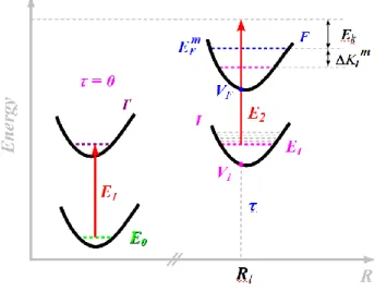
Consider the photoionization process depicted in Figure 1. A N-electrons molecule in the electronic state I and the stationary vibrational level m, with eigenvalue

E

_Im, is excited with a monochromatic laser of fixed energy E. As a result, an electron with asymptotic kinetic energy

2 2

/ 2

k e

E

=

k

m

(me and k are the mass and wavevector of the photoelectron) is ejected, leaving

the remaining N−1 electron system in the electronic state F and vibrational level n, with eigenvalue

n F

E

.

Figure 1. Schematic representation of the photoionization for the steady case.

From a semiclassical standpoint, the probability of occurrence of such a process is proportional to the cross section per unit of electron kinetic energy:

( ) (

)

(

( )

( )

)

( , _k) _{Im IF} , _k, _{k IF mn} ,

F

E E d   E E  E E V K

 =



R R R − +  R +  R (1)

where _Imis the probability distribution of nuclear coordinates R for the source state I,m , _IF

is the photoionization cross section between I and F, and the delta function imposes the energy resonance condition involving the ionization potential V_IF =V_F − and the kinetic energy V_I

6 difference K_mn =E_n−E_m between the two states. The sum runs over all target F states contributing to the process.

Supposing that the photoprocess is instantaneous and that the nuclear momentum does not change, K_mn . Additionally, replacing the 0 

( )

x function by a sharp function, one obtains

( )

(

)

( )

( , _k) _{Im IF} , _k, _{s k}, _IF , ,

F

E E d   E E w E E V 

 



R R R _ −  R _ (2)

where w is given either as a normalized Gaussian _s





_{( ) (}

1/

₎

(

₍

(

₎

)

)

2 2 2 1 exp for , , , _{2 / 2} 0 for , 2 / 2 k IF k IF s k IF k IF E E V E E V w E E V E E V  _{  }  _{− − − }      −   −  =_       −   (3) or a normalized Lorentzian





(

)

₍

₍

(

₎

)

₎

₍

₎

2 2 2 / 2 1 for , / 2 , , _{/ 2} 0 for . k IF s k IF _{k IF} k IF E E V w E E V _{E E V} E E V        −   −  = − −  +   −   (4)

In both cases,



is an arbitrary parameter determining the line width. It should be much smaller than the band width to not interfere with the results, usually  1 eVis enough to satisfy this requirement.

2.1.1 Nuclear ensemble approach for steady spectra

The integral over R in Eq. (2) can be solved by a Monte-Carlo procedure, leading to

(

)

( )

1 1 ( , ) = , , , , , p N k IF k l s k IF l F p l E E E E w E E V N =   

 

R _ −  R _ (5)

where a set of

N

_p nuclear geometries R are generated according to the _l _Im distribution. In the particular case when the system is prepared before the ionization in the electronic and vibrational ground states I =0 and m =0, it is fair to assume that the harmonic approximation is valid. Under these conditions, it is more natural,2b _{as well as numerically efficient, to perform}

7 the sampling of the nuclear configurations in the normal mode coordinates q, where the nuclear ensemble is defined by the marginal Wigner distribution function for the quantum harmonic oscillator22 1/ 2 2 00 1 ( ) exp . d N i i i i i i q       =     = _{  }− _    



q (6)

Here, _i is the angular frequency associated with the ith normal mode with reduced mass μi. Nd is

the number of normal modes in the system. Once Np nuclear geometries ql are generated according

to

 q

₀

( )

, they are transformed back to Cartesian coordinates Rl.

2.2 Time-resolved PE spectra

Suppose now that the molecule is at time t = 0 in the electronic and vibrational ground state, with energy E0, when a laser of energy E1 pumps it to the excited state I'. This first excitation is

considered fully vertical, so that the nuclear coordinates and conjugate momenta remain constant. Once in the I' state, the system is allowed to evolve freely and, at t= , the dynamics is probed by 

ionizing the molecule with a second laser of energy E2, exactly under the same conditions as in

Section 2.1. As nonadiabatic transitions are allowed during the dynamics, the electronic state I at the moment of the ionization, with total energy

E

_I

= +

E

₀

E

₁, may in general be different of I'. This is schematically depicted in Figure 2.

Given the equivalence, the analysis of this time-resolved situation parallels the development of the steady case, considering that the effects of the two laser pulses are uncorrelated. Nevertheless, there are some fundamental differences: first, the nuclear state of the molecule at t = τ is described by a wavepacket, not by a single stationary state; second, the laser pulse duration is in the femtosecond scale, impacting the energy resolution.

Bennett et al.3 have shown that the time-resolved case can still be written analogously to Eq. (5), but with the initial ensemble distribution given by the population I





of state I at time . The photoelectron spectrum is then given by

( )

(

)

(

( )

)

( )

2 2 2 ( , _k, ) = _{I IF} , _k, _{s k}, _IF , . F E E  d    E E  w E E V  



R R R _ −  R _ (7)

8 This approximation, which like in the steady case still assumes that the nuclear momentum does not change, implies that the electron is always ejected with the maximum allowed kinetic energy,

max , 2

k IF IF

E =E − V .

Figure 2. Schematic representation of the photoionization for the time-resolved case.

Because the molecule at time



is described by a wavepacket rather than by a stationary eigenvector of state I, the Franck-Condon overlaps between I and F are much more complex than in the steady case.19b Therefore, to assume that the nuclear momentum remains constant during the photo-transition (E_{k IF}max_, ejection) may be too restrictive. To go beyond this hypothesis, we have also tested a model that simply assumes that any value between E_{k IF}max_, and

E

_kmin

=

0

is equally probable (from the vibrational point of view). In this case, the

w

s function in Eq. (7) should be

replaced by a normalized rectangular function allowing for contribution in the whole domain:



 (

2

)

1 2 2 2 for , , 0 for . IF k IF r k IF k IF E V E E V w E E V E E V −  _{−   − }  −  _{= }  −   (8)

With this new assumption, which has also been applied by Fuji et al.,10a the semiclassical expression for the time-resolved spectrum is

( )

(

)

(

( )

)

( )

2 = 2 2 ( , _k, ) _{I IF} , _k, _{r k}, _IF . F E E  d    E E  w E E V 



R R R _ −  R _ (9)

9 In the remaining paper, when using sharp w functions, we will refer to it as the peaked _s

vibrational background (PVB) model; when using rectangular w functions, we will refer to it as _r

the constant vibrational background (CVB) model.

2.2.1 Nuclear ensemble approach for time-resolved spectra

Either with Eq. (7) or with Eq. (9), the integral over R is solved by a Monte-Carlo procedure, leading to

( )

(

)

(

( )

)

1 1 ( , , ) = , , , , p N k IF k l k IF l F p l E E E E w E E V N     =   

 

R _ −  R _ (10)

where a set of

N

_p nuclear geometries R are generated according to the _l I





distribution.

In practical terms, the nuclear ensemble



_I

( )

R

at time t = τ is built by first running a conventional surface hopping simulation,23 _{and then collecting geometries R within a time window}

t

   +   after the photoexcitation. For each R, IF is computed for max

,

k IF

E in the case of Eq. (7) or for n values of _li E regularly spaced between zero and _k

E

₂

− 

V

_IF in the case of Eq. (9). For evaluation of  , we search this grid for the values immediately inferior

( )

n 1

k

E − and superior

( )

n k

E

to E , and compute _k  with the linearly-interpolated cross section

( )

( )

1

( )

₍

( )

₎

1

(

1

)

1 . n n IF k IF k n n IF k IF k n n k k k k E E E E E E E E     − − − − − = + − − (11) 2.3 Cross sections

From the light-matter interaction theory up to first order and in the electric-dipole approximation, it is possible to show that the state-resolved photoionization cross section for this process is given by the expression24 2 0 ( , , ) kn( ) , IF E Ek E DIF c    R = R (12)

10 where



₀ is the vacuum permittivity and c is the speed of light. The quantity kn

( )

IF

D

R

denotes the photoelectron transition dipole matrix element as a function of the nuclear coordinates R, formally defined as ˆ ( ) ( ; ) | · | ( ; ) , n n k k IF F I D R =  r R μ e  r R  (13)

where

 r R

_I

( ; )

and

 r R

k_F

( ; )

are the corresponding electronic wavefunctions before and after the ionization. Note that



k_F also describes the ejected electron with wavevector k . The remaining

terms in Eq. (13) are the electric dipole operator μ and the unit vector ˆe in the direction of the electric field of the laser. Integration in Eq. (13) is over the electronic coordinates r.

Usually, the transition dipole matrix is computed within the Condon approximation at the nuclear equilibrium geometry R . The nuclear ensemble, however, is intrinsically a post-Condon ₀

approach, as the transition moments are by construction computed for a distribution of nuclear geometries. For this reason, working equations are derived here implicitly retaining the dependence of

D

_IFk on R .

Now, assuming the photoelectron ejection is fast, the final electronic state can be represented by the uncorrelated product17

, k k F FF  =  (14) k F



is the wavefunction of the ejected electron and



_F the electronic wavefunction describing the F state of the remaining N −1 electron species. Also assuming that



_Fk is orthogonal to the orbitals of the initial state (strong orthogonality conditions), then

2 2 ˆ | · | . N k k d IF F IF D =  μ e  _r (15)

Integration in Eq. (15) is over only one electron coordinate,

r

_N in this case.



_IFd

( )

r

_N is the Dyson orbital (DO) associated with the particular I→F transition, formally defined as25

1 { } ( ) | , N d IF N N F I  r =   _{r −} (16)

11 where the integration is here over the remaining N −1 electron coordinates. Note that



_IFd is defined for a given nuclear configuration

R

. Introducing the norm of the Dyson orbital d

IF  , Eq. (15) can be rewritten as 2 2 2 ˆ | · | , N k d k d IF IF F IF D =   μ e _r (17)

where _IFd =_IFd / _IFd is just the DO normalized to one.

Once the DOs and their norms are known, the right-hand side of Eq. (17) can be evaluated. In this work, after computing the DOs as explained later in Section 2.4, we have used the EZDYSON

3.2 program16c, 17 to compute IF

( )

Rl . This program offers the options of representing k F



on a basis set of Spherical or Coulomb partial waves,26 and also includes isotropic angular averaging of the photoelectron dipole matrix elements. The free electron states are represented by16a, 16b

( )

1/ 2 1/ 2

( )

, k e F k m k F  r = r (18)

where F R is the electron wave expansion in a convenient basis and _k

( )



_Fk is normalized to energy interval (i.e., it has units of (volume × energy)-1/2). Thus, the transition moment is

2 2 2 2 | | . 3 N k e d d k I IF IF F IF m g D = k     _r (19)

The factor 1/3 stems from the isotropic averaging, whileg accounts for spin and orbital _I

degeneracies of state I. Replacing Eq. (19) into Eq. (12) renders

0 2 2 3 | | . 3 N d d e I IF IF k IF m k E F g c       =  _r (20)

In addition to simulations based on the full computation of the cross sections, we have also simulated the spectrum based on a second approach, which consists of simply approximating Eq. (20) to 2 , d IF C IF    (21)

12 where C is an arbitrary constant. In this case, all functional dependence of the transition dipole moments on the geometries and final states are supposed to be contained in the DO norms.

In the remaining text, when using Eq. (20) to simulate the spectrum, we will refer to it as the cross section approach, and when using Eq. (21), as the DO norm approach.

2.4 Dyson orbitals

The DO associated with a particular I → F transition (Eq. (16)) is a single electron wavefunction containing information on where the ejected electron was removed from. According to our previous developments, once the DOs are known, the cross sections can be evaluated and the photoelectron spectrum fully computed. In the Supporting Information (SI-1), we provide a detailed discussion on how to compute DOs. Here, we will outline only few key aspects.

As shown in the SI, Eq. (16) can be rewritten as a linear combination of spin-orbitals



_q as 1 ( ) ( ), b f N d IF N s s N s b   = =



r r (22) with max N 0 1 , N q s n j qs n j b d  = = =

 

(23)

where



_qs is the Kronecker delta function. The coefficients

max M 0 ( 1) | . q N j j n j n m m n m d + c c = = −



   (24)

are computed in terms of Slater determinant overlaps   _m| _nj and configuration interaction (CI) coefficients c and _n c defining the electronic wavefunctions of the N and N-1 electron systems, _m

respectively. To reduce computational costs, d terms with expansion coefficient _{n j}q

c

n or

c

m

smaller than an arbitrarily small value _cis can be neglected. In all results discussed here, we have adopted _cis =0.01.

13 Using Eq. (22), the DO norm can be easily computed as

1/ 2 2 1 , b f N d IF s s b  =   = _ _ 



 (25)

which, in general, is not equal to one. In fact, d IF

 may range from 0 to 1 and, as can be inferred from Eq. (21), it is a measure of the photoelectron ejection probability.27 _{The closest the norm to}

0 (1) the less (more) probable the ionization.

While, the Slater determinant overlaps required in Eq. (24) can be readily computed in terms of the overlap matrix between atomic orbitals

S

_uv

= 

 

_u

|

_v



, a standard output when computing the electronic states, the CI coefficients in the framework of linear-response TDDFT requires some additional discussion, which is done in the next section.

2.4.1 Dyson orbitals with TDDFT

The theory presented so far in this section to compute the DOs is general and can in principle be applied for any method used to solve the electronic problem. The only condition is the representation of the electronic wavefunctions as a linear combination of Slater determinants. Within the frame of Hartree-Fock based methods, that introduces no problem as it is a common assumption of the methodology. Therefore, the expansion coefficients

c

_n and

c

_m are directly computed. In the case of TDDFT, approximated wavefunctions in the CI form should be built.

According to the Casida's Ansatz for state assignment,28 the electronic wavefunction corresponding to a given excited state K can be represented as

, K K ov ov o v C  =



 (26)

where o and v stand for occupied and virtual spin-orbitals of the same spin, respectively. Denoting by



₀ the Kohn-Sham Hartree-Fock ground state determinant,



_ov are singly excited Slater determinants, where the oth occupied spin-orbital has been replaced by the vth virtual one of the same spin, analogous to a configuration interaction with single excitations. Notice that only excited

14 Slater determinants are included in Eq. (26). The ground state wavefunction is by definition

0 0

 = 

.

The use of Eq. (26) for building wavefunctions out of TDDFT amplitudes has become very popular recently.29 _{It has been extensively used for computations of nonadiabatic couplings in}

dynamics simulations30 _{and also employed to compute different types of quantities, including}

spin-orbit couplings,31 _{transition dipole moments,}10b, 32 _{nonadiabatic coupling vectors,}32-33 _{and Dyson}

orbitals.8b In fact, this same methodology has been generalized34 to build wavefunctions to other linear-response-based methods as well, like ADC(2) and CC2.35

The expansion coefficients in Eq. (26) can be explicitly computed as28

1/ 2 ( ), K v o K K ov K ov ov K C A X Y E    −  = _{ } +    (27)

where  is the transition energy E_K

0, K VK V

E

 = − (28)

o



(



_v) is the energy of the molecular orbital o (v), and K + K

X Y is the linear response TDDFT vector associated with the Kth electronic state. The remaining term,

1/ 2 2 , | K | , K ov o v A C −   =   



 (29)

is a normalization factor introduced to ensure electronic wavefunctions normalized to unity.

3

Steady PE spectra of imidazole and adenine

According to the developments of Section 2.1, calculation of the steady spectrum at a given value of kinetic energy Ek of the photoelectron can be pictured in three main steps: (i) generation of the

nuclear ensemble; (ii) calculation of the DOs and IPs for each nuclear configuration and F electronic state considered; and (iii) calculation of the individual photoelectron intensities, from which the full spectrum is statistically computed. Along this section, we will illustrate each of these steps when applied to the He(I) photoionization of imidazole20c and adenine.20b

15

3.1 Nuclear ensemble

The steady PE spectra of imidazole and adenine were computed at E = 21.21 eV, which corresponds to the energy of a He(I) source. As the ionization is assumed to occur from the electronic and vibrational ground states, the nuclear configurations were sampled according to Eq. (6). An ensemble of Np = 500 nuclear geometries was generated in normal modes coordinates for

each molecule and then transformed back to Cartesian coordinates. The equilibrium geometries

R0, normal mode frequencies ωi, and normal mode eigenvectors were computed at

B3LYP/aug-cc-pVTZ level. DFT and TDDFT calculations here, as in rest of the paper, were all performed with GAUSSIAN 09.36

3.2 IPs and DOs

For each nuclear configuration, the electronic ground state of the neutral molecules was computed within DFT at CAM-B3LYP/aug-cc-pVDZ level. The first 40 states of imidazole cation and the first 10 of adenine cation were considered. All those doublet excited states were computed within TDDFT with the same functional37 _{and basis set.}38

After building approximated electronic wavefunctions for all these states, the DOs corresponding to each particular I = 0 (neutral) → F (cation) transition were computed according to the formalism presented in Section 2.4. To illustrate this step in more details, Table 1 (imidazole) and Table 2 (adenine) present the values of V_0F and ₀d

F

 for the corresponding equilibrium geometries of each system, together with the experimental IPs for each molecule.20b,

20c

As can be seen from the tables, theoretical IPs are in excellent agreement with experimental ones. Another interesting feature that can be appreciated is that although all 0 → F transitions are energetically allowed (V_0F  ), not all of them contribute to the spectrum. For imidazole, for E

instance, only a few transitions really do so, the rest being practicably negligible, given their small DO norms. Moreover, among the significant transitions, we can find very intense ones (norms close to one), like the 0 → 0 in both molecules, and some much less intense, like the 0 → 9 for imidazole or 0 → 7 for adenine. Thus, with DO norms alone, one can not only identify which

16 transitions really contribute to the spectrum, but also what the relative contribution from each transition will be.

Table 1. IPs (in eV) and DO norms ₀d F

 corresponding to each 0 → F transition for the equilibrium geometry of imidazole. The experimental IPs reported in ref.20c are given as well.

F



V

₀exp_F t V0 F

( )

R0 0

( )

0 d F  R _F



V

₀exp_F t V0 F

( )

R0 0

( )

0 d F  R 0 8.81 8.99 0.98 20 18.08 18.23 0.79 1 10.38 10.30 0.96 21 18.30 0.07 2 10.62 0.91 22 18.33 0.02 3 14.03 14.07 0.96 23 18.90 0.18 4 14.21 0.70 24 18.94 0.00 5 14.74 0.27 25 18.95 0.17 6 14.77 14.93 0.91 26 18.98 0.20 7 15.38 15.04 0.96 27 20.48 19.04 0.73 8 15.15 0.10 28 19.17 0.01 9 15.25 0.33 29 19.19 0.13 10 15.40 0.33 30 19.24 0.01 11 16.05 0.20 31 19.28 0.19 12 16.13 0.13 32 19.36 0.00 13 16.71 0.34 33 19.39 0.12 14 16.92 0.14 34 19.39 0.00 15 17.49 0.08 35 19.52 0.37 16 17.92 0.10 36 19.53 0.03 17 18.10 0.13 37 19.54 0.03 18 18.13 0.02 38 19.55 0.32 19 18.16 0.00 39 19.59 0.05

Table 2 also shows OVGF results for adenine.20g _{As this method is one of the most reliable}

approaches for determination of IPs, they help to gage the quality of the current TDDFT results. Up

to 12 eV (D6), these two data sets are in excellent agreement with each other, with a RMSD of 0.2

eV for the IPs. Above 12 eV, however, the agreement is not as good; TDDFT distributes the intensity of the 13.21 eV experimental band over three low-intensity states (D7-D9), while OVGF

17 Table 2. IPs (in eV) and DO norms ₀d

F

 corresponding to each 0 → F transition for the equilibrium geometry of adenine. Experimental IPs reported in ref.20b and OVGF/6-311++G** data from ref.20g are given as well.

TD-CAM-B3LYP OVGF a F



V

₀exp_F t V0 F

( )

R0 0

( )

0 d F  R V_{0 F}

( )

R₀ P1/2 0 8.48 8.35 0.98 8.32 0.95 1 9.58 9.51 0.94 9.40 0.94 2 9.69 0.87 9.45 0.94 3 10.50 10.45 0.95 10.50 0.94 4 10.62 0.88 10.53 0.94 5 11.39 11.37 0.93 11.61 0.94 6 12.10 12.02 0.80 12.28 0.93 7 13.06 0.32 8 13.24 0.11 9 13.21 13.48 0.52 13.63 0.92 a

P1/2 _{is the square root of the OVGF intensity.}

3.3 Steady PE spectrum

Once IPs and DOs (Eq. (22)) are computed for each nuclear configuration Rl of the ensemble (Eq.

(6)) and for F electronic state of the cation, the spherically averaged total cross section for the same geometries (_IF

( )

R_l , Eq. (20)) are computed, and the spectrum is simulated (Eq. (5)).

( )

IF l

 R are computed with the EZDYSON 3.2 program. The free-electron wavefunction was expanded in Coulomb partial waves to an angular momentum of lmax = 6, which we found out to

be enough to converge the ionization probabilities. The photoelectron dipole matrix elements were averaged over all molecular orientations, which is justified by the non-polarized character of the laser used in the experiments and the random orientation of the molecules before the ionization. Alternatively, we have also computed the spectrum based on the DO norm approach, using Eq. (21).

18 Figure 3. Simulated (this work) and experimental20c steady PE spectra of imidazole for a laser energy of 21.21 eV. The intensities of the experimental spectrum and of the simulation based on DO norms are normalized to match the maximum of the first peak. Bottom: Individual contributions from each cationic state up to D39; the dotted line shows the sum over all components.

0.1

 = eV.

The simulated PE spectra obtained by both approaches, cross section and DO norm, are shown in Figure 3 for imidazole and Figure 4 for adenine. Experimental results from refs.20b, 20c are shown as well. All curves are represented as a function of the binding energy, defined as

b k

E = −E E . As can be seen in the figures, the theoretical methods are able to correctly reproduce both the position and width of the bands. The relative intensity of the bands shows some dependency on the method, but a nice agreement with the experiment is in general reached. For imidazole, the DO norm approach renders the medium and high energy bands at 14 and 18 eV with too low intensities, as compared to the low energy bands. The full computation of the

8 10 12 14 16 18 20 0 20 40 60 8 10 12 14 16 18 20 0 20 40 60 Experiment Simulated DO norms Simulated cross section

In te n sit y ( M b .e V -1 )

Binding energy (eV)

D₂₄-D₃₉ D₇-D₁₂ D₀ D₁₅-D₂₃ D₁₃D₁₄ D₄-D₆ D₁D₂ D3 In te n sit y ( M b .e V -1 )

19 transition moments in the cross section approach tends to deliver better balanced relative intensities.

Figure 4. Top: Simulated (this work) and experimental20b steady PE spectra of adenine for a photon energy of 21.21 eV. The intensities of the experimental spectrum and of the simulation based on DO norms are normalized to match the maximum of the first peak. Bottom: Individual contributions from each cationic state up to D9. The dotted line shows the sum over all components.

0.1

 = eV.

Concerning intensity, only the cross section approach can provide absolute values. In Figure 3 and Figure 4, the intensities of the spectra based on DO norms are normalized to match the intensity of the first peak of the spectra based on cross sections. Unfortunately, absolute intensities for these molecules have not been experimentally reported, and the same normalization procedure was applied.

8 10 12 14 0 20 40 60 80 100 120 8 10 12 14 0 20 40 60 80 100 120 Experiment Simulated DO norms Simulated cross section

In te n sit y ( M b .e V -1 )

Binding energy (eV)

D₇ -D₉ D₆ D₅ D₁ D₂ D₃ D₄ In te n sit y ( M b .e V -1 )

Binding energy (eV)

20 The good agreement between the spectra computed with cross sections and DO norms in the low binding energy region implies that the cross section approximation in Eq. (21) is valid for

IF

E V . Thus, as long as absolute intensities are not required, the low-energy region of the photoelectron spectrum may be simulated with the DO norm approach, significantly reducing computational costs.

The bottom graphs of Figure 3 and Figure 4 show the contribution of each S0→Dn transition

to the total cross section. For both molecules, only few cation states contribute to the spectrum up to 14 eV. In some cases, a single experimental band may correspond to the overlap of transitions into more than one state, as for instance transitions into D1 and D2 forming the second

photoelectron band of the two molecules.

Above 14 eV, the number of states needed to compute the spectrum increases substantially. For imidazole, for instance, transitions into nine states (D3 to D12) contribute to the broad band

starting at 13 eV. For the next band starting at 18 eV, even considering 24 states (D15 to D39), we

have not been able to reproduce the experimental band shape. This large demand for states in the high energy region points to a major limitation of the method. Not only the simulation costs may be prohibitive, but also the computed properties of such highly excited states are not fully reliable, especially within linear-response approximation.

4

Time-resolved PE spectra of imidazole

As in the steady case, the calculation of the time-resolved PE spectrum at a given Ek can also be

pictured in three main steps: (i) generation of the nuclear ensemble, (ii) computation of the DOs and IPs, and (iii) calculation of photoelectron intensities, from which the spectrum is statistically computed. However, according to the developments of Section 2.2, step (i) is fundamentally different now: the nuclear ensemble has to be selected from nonadiabatic dynamics. Along this section, we illustrate all these steps, when applied to simulate the time- and kinetic-energy-resolved PE spectrum of imidazole.

21

4.1 Nuclear ensemble from surface hopping

As imidazole is initially pumped from the vibrational ground state, the sampling of the nuclear coordinates and conjugate momenta at t = 0 was performed according to a Wigner distribution function for S0. The same R0, ωi, and normal-mode eigenvectors as in Section 3.1 were used. A

set of 500 nuclear configurations and conjugate momenta were generated and projected onto the adiabatic electronic states to compute the absorption spectrum shown in Figure 5.

In the experimental setup,8d a pump laser of energy E1 = 6.18 eV (200.8 nm) was used to

directly excite imidazole from the electronic ground state into the 1ππ* state. From the computational side, using TDDFT at CAM-B3LYP/aug-cc-pVDZ level, we found out that the simulated absorption spectrum is blue-shifted by 0.2 eV compared to the experimental spectrum20a (Figure 5). Therefore, to excite the 1ππ* state of imidazole in the same region as done in the experiments, an energy E1 = 6.4 eV is necessary in the computational modelling. This value was

used in the simulations.

Figure 5. Simulated and experimental20a absorption spectrum of imidazole in the gas phase. The intensity of the experimental spectrum was normalized to match the simulated one.

To initiate the dynamics, 500 phase-space points sampled for the absorption spectrum were screened to select those with excitation energy E_I −E₀ within the narrow energy interval E1 ± 0.1

eV, and resampled using their corresponding oscillator strength as transition probability.2b A set

5 6 7 0 20 40 60 Theory Fitting Experiment Fitting Ph oto ab so rpt io n c ros s s ec tio n (M b) Photoenergy (eV)

22 of 100 points matching these energy-window and oscillator-strength criteria was selected to be used as initial conditions for trajectories.

The number of initial conditions per adiabatic electronic state is shown in Table 3. This distribution reflects the geometric distortions in the sampling. Although the vertical excitation into the bright * state is S3 for the equilibrium geometry, Table 3 shows that, depending on the

geometry, this state may shift as down as S2 and as high as S6.

Table 3. Number of initial conditions per electronic state for which E_I−E₀ is within the energy interval E1 ± 0.1 eV.

SI = S1 S2 S3 S4 S5 S6 S7 Total

0 26 46 21 6 1 0 100

The electronic energies, energy gradients, and nonadiabatic coupling terms were computed ‘on-the-fly’ within the frame of TDDFT at CAM-B3LYP/aug-cc-pVDZ level. Excited electronic states up to S8 were included in the dynamics. Each trajectory was propagated for a maximum of t = 500 fs, with an integration step of 0.5 fs for classical equations and 0.025 fs for quantum

equations.

Nonadiabatic transitions between different electronic states were treated with the fewest-switches surface hopping39 including decoherence corrections ( = 0.1 Hartree).40 Nonadiabatic couplings with TDDFT were computed by finite differences with the method discussed in ref.30a, which is based on the Hammes-Schiffer/Tully approach.41 As a single-reference method, TDDFT cannot provide reliable nonadiabatic couplings for crossings with the ground state. For this reason, when a trajectory reached an S1-S0 energy gap smaller than 0.15 eV before the maximum

simulation time, it was stopped. This procedure did not affect the spectrum simulations, as at this point the probe energy was already smaller than the ionization energy.

After completing the dynamics, trajectories were split in regular intervals of  = 25 fs starting from  = 0. For each time interval i between 0 and the maximum simulation time, Np =

500 nuclear geometries

R

( )_li were randomly selected from the trajectories and used to compute the spectrum.

23 Initial conditions, semi-classical dynamics, absorption spectrum, and photoionization spectrum were computed with NEWTON-X interfaced with GAUSSIAN 09.

4.2 IPs and DOs

According to ref.8d, a laser of E2 = 4.93 eV (251.6 nm) was used in the experiment to probe the

dynamics after the E1 = 6.18 eV (200.8 nm) pump excitation. In the simulation, for each

R

( )_li , the

DOs and their norms associated with each I → F transition were computed, where I is the current electronic state of the neutral molecule at the moment of the ionization and F are all cation states from 0 to 4.

Table 4. Vertical excitation energies (singlet-singlet; E_0I in eV) and vertical IPs (singlet-doublet; V_IF in eV) computed at the equilibrium geometry R₀. The values of the oscillator

strength (f ) and of the squared DO norm ( _IFd (R₀) 2) are shown in brackets. State assignments in terms of the main orbital contribution are given in parenthesis. cs – closed shell; 3sX – 3s

Rydberg orbital on atom X. 0I E  (eV) [f ] IF V  (eV) [_IFd 2] I/F 0 1 2

D0 (1hole) D1 (nhole) D2 (2hole)

0 S0 (cs) 0.00 8.99 [0.96] 10.30 [0.91] 10.62 [0.83] 1 S1 (3sN) 5.59 [0.000] 3.40 [0.47] 4.71 [0.00] 5.02 [0.00] 2 S2 (3sC) 6.36 [0.030] 2.64 [0.47] 3.95 [0.00] 4.26 [0.00] 3 S3 (*) 6.43 [0.169] 2.56 [0.42] 3.87 [0.00] 4.19 [0.01] 4 S4 (3sC) 6.63 [0.000] 2.36 [0.38] 3.67 [0.00] 3.99 [0.00] 5 S5 (n*) 6.72 [0.004] 2.28 [0.00] 3.59 [0.31] 3.90 [0.00] 6 S6 (3sN) 6.99 [0.002] 2.00 [0.00] 3.31 [0.00] 3.62 [0.36]

Before proceeding with the spectrum discussion, it is illustrative to characterize the ionization process for the S0 equilibrium geometryR , which approximately corresponds to the ₀

24 shown in Table 4. As can be seen, only electronic states of the cation up to F = 2 (D2) need to be

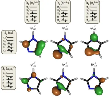
considered for this particular geometry. (In fact, this is also true for all remaining geometries.) The DOs corresponding to ionizations from S0 (closed shell) and S3 (*) are shown in

Figure 6. The main configuration for each singlet and doublet state is schematically shown in the figure as well. The doublet configurations differ from that for S0 by a single spin orbital. Therefore,

according to the ionization rules discussed in the Supporting Information (SI-2), such ionization processes are allowed. This is corroborated by the large DO norms for S0→Dn processes reported

in Table 4. In the case of S3, only ionization into D0 is allowed according to the ionization rules,

which is also corroborated by the results in Table 4. As we discuss below, this ionization pattern from S3 will have major consequences for the simulation of the time-resolved spectrum.

Figure 6. DOs for ionization from S0 (closed shell) and S3 (*) into the first three cation

states (D0 to D2) computed for the equilibrium geometry of imidazole with TDDFT.

4.3 Time-resolved spectrum

Once IPs and DOs are known for each nuclear geometry

R

( )_li between the current state I and F

cation states, the time-resolved PE spectrum can be computed either with the cross section approach (Eq. (20)) or with the DO norm approach (Eq. (21)). Then, if we suppose that the electron is ejected with the maximum kinetic energy, the photoelectron spectrum is computed based on

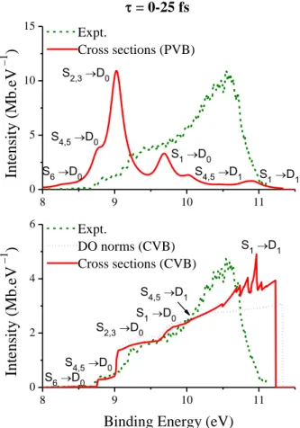
25 peaked line shapes (PVB model), as given by Eq. (7). In Figure 7-top, the simulated spectrum using the PVB model is shown for the early dynamics, collecting configurations generated in the first 25 fs of dynamics simulations. The experimental spectrum from ref.8d for zero time delay is also shown, normalized to the maximum of the simulated result. (For an analysis of the experimental results, see ref.8d, 20d, 20e). The spectra are plotted in terms of the binding energy

1 2

b k

E =E +E −E . Transition dipoles were computed with Coulomb partial waves (lmax = 6)

between the current neutral state at a certain time step and all cation states up to F = 4 (D3). The

line width was assumed to be  =0.2 eV.

Figure 7. Photoelectron spectrum for configurations sampled within the first 25 fs of the dynamics simulations. Top: Spectrum based on the PVB model. Bottom: Spectrum based on the CVB model. In both cases, experimental data from ref.8d _{are shown. Different normalizations of}

experimental data are applied in each panel (see text).

8 9 10 11 0 5 10 15 8 9 10 11 0 2 4 6 S₁→D₁ S_4,5→D₁ S₁→D₀ S_2,3→D₀ S_4,5→D₀ S₆→D₀  = 0-25 fs Int ensi ty (M b.eV − 1 ) Expt. Cross sections (PVB) S₁→D₁ Int ensi ty (M b.eV − 1 )

Binding Energy (eV)

Expt. DO norms (CVB) Cross sections (CVB) S_4,5→D₁ S₁→D₀ S_2,3→D₀ S_4,5→D₀ S₆→D₀

26 It is clear from Figure 7-top that the spectrum computed with the PVB model poorly compares to the experimental result. The simulation has several peaks at the resonant points defined by E_b =E₁+E₂−E_{k IF}max_, =E₁+ V_IF, with the main contribution coming from ionization of S2 and S3 into D0. The experimental spectrum, on its turn, is much broader and it peaks at much

larger binding energies than predicted by the simulation.

The large biding energy in the experimental data shown in Figure 7-top implies that electrons are being ejected with low kinetic energies, which has been attributed by Humeniuk et al.8b to a rearrangement of the nuclear wavepacket due to its interaction with the probe pulse. This also means that the hypothesis underlying the PVB model, i.e. that electrons are ejected at the maximum kinetic energy, does not hold in the present case and simulations based on the CVB model may be more adequate. In Figure 7-bottom, we show the spectrum simulated with this model, as given by Eq. (9), for times smaller than 25 fs. As before, transition dipoles were computed with Coulomb partial waves (lmax = 6) between the current neutral state and all cation

states up to F = 4. n =_li 10 points were used in the linear interpolation of Eq. (11). The experimental spectrum from ref.8d for zero delay is also shown, but now normalized to the intensity of the S4 →

D0 contribution.

The agreement of the CVB model with the experiment is still not perfect, but it is significantly better than with the peaked model. The simulation correctly predicts a series of substructures in the spectral intensity distribution. As shown in Figure 7-bottom, the trace of the experimental spectrum at  = 0 exhibits inflexion changes at 8.7, 9.2, and 10 eV. The simulation shows equivalent inflection changes at 8.7, 9.0, and 9.7 eV. The data analysis revealed that they are related to which neutral states are contributing to the ionization. Below 8.7 eV, only ionization into D0 coming from S6 contributes to the spectrum. Above this value, D0 ionization of S4 to S5

also contributes causing the spectral shift. Starting from 9.0 eV, ionization of S2 and S3 into D0

starts to contribute. S1 ionization appears at above 9.7 eV. A small contribution from ionization of

S4 and S5 into D1 is observed above 10 eV.

The early dynamics spectrum computed with the DO norm approach and the CVB model is also shown in Figure 7-bottom. It is normalized to match the cross-section based spectrum at the S4 → D0 contribution. The agreement between the two approaches is very good, once more

27 computation of the cross sections. The main difference between the two approaches comes is in the slope of the spectra for large binging energies. It is caused by a small effective near-linear dependence of the transition dipole on the electron kinetic energy, which is completely neglected in the DO norm approximation.

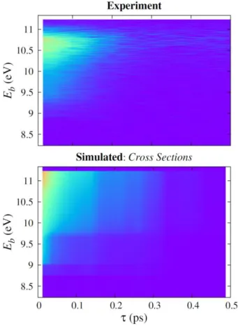
The time evolution of the spectrum using the CVB model with the cross section approach is shown in Figure 8. The sub-picosecond time distribution of the spectrum is well predicted. In particular, the simulation clearly reproduces the dependence of the time decay on the binding energy, with a systematic increase of the lifetime between 9 and 11 eV.

Figure 8. Time- and kinetic-energy-resolved PE spectrum of imidazole. Top: Experimental data from ref.8d; Bottom: simulations using the CVB model and the cross section approach. The intensities were renormalized to match each other at  = 0 and Eb = 9 eV.

In spite of the qualitative agreement between experiment and simulation with CVB model, the predictions for the binding energy distribution are, however, not entirely satisfactory. While

28 the experimental spectrum peaks at 10.5-10.7 eV and quickly drops to zero before the maximum biding energy (11.33 eV), the simulations do not show this important feature, but only a flat plateau extending up to the maximum binding energy (this is better seen in Figure 7-bottom). The reason underlying this difference can be traced back to three factors. First, the CVB model itself, which, as already discussed, provides only a very approximated guess on how vibrational overlaps modulate the distribution of electron kinetic energies. Second, the experimental setup in which electrons with small kinetic energy are not fully collected, causing the intensity drop before the maximum binding energy. Third, a TDDFT failure to describe the multiconfigurational character of the * state of imidazole. This last point is discussed next.

We know from CASPT2 calculations for imidazole that the * state has strong contributions from 1* and * configurations (see, for instance, ref.42). This

multiconfigurational character plays a central role for the spectrum, splitting the ionization signal in two components, depending on whether the hole is created in the 1 or  orbital. The 1hole,

which is formed after ejection of the electron in the 1* orbital (approximately the DO



₃₀d in

Figure 6), leads to an ionization signal spanning from E_bmin = V₀₀=8.99 eV (see Table 4) to max

1 2

11.33 eV

b

E

= +

E

E

=

. On the other hand, the 2hole, formed after electron ejection from 2*

(the DO



₃₂d ), leads to ionization signals from E_bmin = V₀₂=10.62 eVto again

E

_bmax

=

11.33 eV

. Thus, the sum of the two components creates a bias towards large E values. TDDFT, on its turn, _b

represents the * state in terms of excitations from 1 only. Therefore, only 1 holes are created,

flattening the result in the 10.5-10.7 eV region.

5

Conclusions

We have implemented semiclassical methods based on the nuclear ensemble approach to simulate steady and time-resolved photoelectron spectra. The current implementation in the NEWTON-X

program works with TDDFT provided by GAUSSIAN 09, but the methods are rather general and

can be easily adapted to work with other electronic structure levels and programs.

For both, steady and time-resolved photoelectron spectra, we have developed and tested two levels of approximations, one based on full computation of transition dipole moments (cross

29 section approach) and another based on an approximation of the transition dipole moments by Dyson orbital norms (DO norm approach). Moreover, the vibrational modulation of the electron kinetic energy distribution was also modeled with two different approaches. In the first one, vibrational overlaps between N and N-1 electron systems were supposed to be significant only for the electrons ejected with the maximum allowed kinetic energy (PVB model), a common approximation resting on the sudden-ionization hypothesis. In the second model, vibrational overlaps were supposed to be constant over the whole electron kinetic energy domain (CVB model).

Applications of the methods have been done for imidazole (steady and time-resolved) and for adenine (steady). The comparison to experimental data shows that steady spectra can be nicely predicted with the PVB model, with good description of intensities and band shapes.

For time-resolved spectra, the PVB model failed and the CVB model rendered significantly better results. The CVB simulations have been able to reproduce a series of substructures in the spectrum, which were assigned to specific ionization processes. Nevertheless, the overall agreement between simulation and experiment was less satisfactory than in the steady case due to the hypotheses underlying the CVB model, the multiconfigurational character of the key state contributing to the spectrum, and the instrumental signal loss not included in the simulations. Considering all hypotheses and approximations invoked, it is truly encouraging that the main qualitative features of the spectrum have been predicted by the nuclear ensemble modelling.

For all tested cases, the approximation of the cross sections by Dyson orbital norms delivered results of similar quality as those based on full computation of cross sections, with an enormous economy of computational effort.

Finally, all these results make us confident that photoelectron spectrum simulations based on the nuclear ensemble approach can be an effective tool to aid deconvolution and assignment of experimental data for large molecules.

Author information

Corresponding author

30

Acknowledgments

MB thanks the support of the A*MIDEX grant (n° ANR-11-IDEX-0001-02) funded by the French Government « Investissements d’Avenir » program. This work was granted access to the HPC resources of Aix-Marseille Université financed by the project Equip@Meso (ANR-10-EQPX-29-01) also within the program « Investissements d’Avenir » supervised by the Agence Nationale de la Recherche. The authors thank C. Angeli and S. Ullrich for discussions.

31

References

1. (a) Barbatti, M.; Granucci, G.; Ruckenbauer, M.; Plasser, F.; Crespo-Otero, R.; Pittner, J.; Persico, M.; Lischka, H., NEWTON-X: A package for Newtonian dynamics close to the crossing seam. Available via the Internet at www.newtonx.org. 2013; (b) Barbatti, M.; Ruckenbauer, M.; Plasser, F.; Pittner, J.; Granucci, G.; Persico, M.; Lischka, H., Newton-X: A Surface-Hopping Program for Nonadiabatic Molecular Dynamics. WIREs: Comp. Mol. Sci. 2014, 4, 26-33.

2. (a) Crespo-Otero, R.; Barbatti, M., Spectrum Simulation and Decomposition with Nuclear Ensemble: Formal Derivation and Application to Benzene, Furan and 2-Phenylfuran. Theor. Chem. Acc. 2012, 131, 1237; (b) Barbatti, M.; Sen, K., Effects of different initial condition samplings on photodynamics and spectrum of pyrrole. Int. J. Quantum Chem. 2015, doi:10.1002/qua.25049.

3. Bennett, K.; Kowalewski, M.; Mukamel, S., Probing electronic and vibrational dynamics in molecules by time-resolved photoelectron, Auger-electron, and X-ray photon scattering spectroscopy.

Faraday Discuss. 2015, 177, 405-428.

4. Petit, A. S.; Subotnik, J. E., Appraisal of Surface Hopping as a Tool for Modeling Condensed Phase Linear Absorption Spectra. J. Chem. Theory Comput. 2015, 11, 4328-4341.

5. Klaffki, N.; Weingart, O.; Garavelli, M.; Spohr, E., Sampling excited state dynamics: influence of HOOP mode excitations in a retinal model. Phys. Chem. Chem. Phys. 2012, 14, 14299-14305.

6. Rivalta, I.; Nenov, A.; Cerullo, G.; Mukamel, S.; Garavelli, M., Ab initio simulations of two-dimensional electronic spectra: The SOS//QM/MM approach. Int. J. Quantum Chem. 2014, 114, 85-93. 7. Polli, D.; Altoe, P.; Weingart, O.; Spillane, K. M.; Manzoni, C.; Brida, D.; Tomasello, G.; Orlandi, G.; Kukura, P.; Mathies, R. A.; Garavelli, M.; Cerullo, G., Conical intersection dynamics of the primary photoisomerization event in vision. Nature 2010, 467, 440-443.

8. (a) Ruckenbauer, M.; Mai, S.; Marquetand, P.; González, L., Photoelectron spectra of 2-thiouracil, 4-thiouracil, and 2,4-dithiouracil. J. Chem. Phys. 2016, 144, 074303; (b) Humeniuk, A.; Wohlgemuth, M.; Suzuki, T.; Mitrić, R., Time-resolved photoelectron imaging spectra from non-adiabatic molecular dynamics simulations. J. Chem. Phys. 2013, 139, 134104; (c) Hudock, H. R.; Martínez, T. J., Excited-State Dynamics of Cytosine Reveal Multiple Intrinsic Subpicosecond Pathways. ChemPhysChem 2008, 9, 2486-2490; (d) Crespo-Otero, R.; Barbatti, M.; Yu, H.; Evans, N. L.; Ullrich, S., Ultrafast Dynamics of UV-Excited Imidazole. ChemPhysChem 2011, 12, 3365-3375; (e) Mori, T.; Glover, W. J.; Schuurman, M. S.; Martinez, T. J., Role of Rydberg States in the Photochemical Dynamics of Ethylene. J. Phys. Chem. A 2012,

116, 2808-2818.

9. McFarland, B. K.; Farrell, J. P.; Miyabe, S.; Tarantelli, F.; Aguilar, A.; Berrah, N.; Bostedt, C.; Bozek, J. D.; Bucksbaum, P. H.; Castagna, J. C.; Coffee, R. N.; Cryan, J. P.; Fang, L.; Feifel, R.; Gaffney,

32 K. J.; Glownia, J. M.; Martinez, T. J.; Mucke, M.; Murphy, B.; Natan, A.; Osipov, T.; Petrović, V. S.; Schorb, S.; Schultz, T.; Spector, L. S.; Swiggers, M.; Tenney, I.; Wang, S.; White, J. L.; White, W.; Gühr, M., Ultrafast X-ray Auger probing of photoexcited molecular dynamics. Nat Commun 2014, 5, 4235. 10. (a) Fuji, T.; Suzuki, Y.-I.; Horio, T.; Suzuki, T.; Mitric, R.; Werner, U.; Bonacic-Koutecky, V., Ultrafast photodynamics of furan. J. Chem. Phys. 2010, 133, 234303-9; (b) Mitrić, R.; Petersen, J.; Wohlgemuth, M.; Werner, U.; Bonačić-Koutecký, V.; Wöste, L.; Jortner, J., Time-Resolved Femtosecond Photoelectron Spectroscopy by Field-Induced Surface Hopping. J. Phys. Chem. A 2011, 115, 3755-3765; (c) Stanzel, J.; Neeb, M.; Eberhardt, W.; Lisinetskaya, P. G.; Petersen, J.; Mitrić, R., Switching from molecular to bulklike dynamics in electronic relaxation of a small gold cluster. Phys. Rev. A 2012, 85, 013201.

11. (a) Wolf, T. J. A.; Kuhlman, T. S.; Schalk, O.; Martinez, T. J.; Moller, K. B.; Stolow, A.; Unterreiner, A. N., Hexamethylcyclopentadiene: time-resolved photoelectron spectroscopy and ab initio multiple spawning simulations. Phys. Chem. Chem. Phys. 2014, 16, 11770-11779; (b) Tomasello, G.; Humeniuk, A.; Mitrić, R., Exploring Ultrafast Dynamics of Pyrazine by Time-Resolved Photoelectron Imaging. J. Phys. Chem. A 2014, 118, 8437-8445.

12. (a) Cederbaum, L. S.; Domcke, W.; Schirmer, J.; Niessen, W. v., Many-Body Effects in Valence and Core Photoionization of Molecules. Phys. Scr. 1980, 21, 481; (b) Ortiz, J. V., A nondiagonal, renormalized extension of partial third-order quasiparticle theory: Comparisons for closed-shell ionization energies. J. Chem. Phys. 1998, 108, 1008-1014; (c) Herman, M. F.; Freed, K. F.; Yeager, D. L., Analysis and Evaluation of Ionization Potentials, Electron Affinities, and Excitation Energies by the Equations of Motion—Green's Function Method. Adv. Chem. Phys. 1981, 48, 1-69; (d) von Niessen, W.; Schirmer, J.; Cederbaum, L. S., Computational methods for the one-particle green's function. Comput. Phys. Rep. 1984,

1, 57-125.

13. Nguyen, N. L.; Borghi, G.; Ferretti, A.; Dabo, I.; Marzari, N., First-Principles Photoemission Spectroscopy and Orbital Tomography in Molecules from Koopmans-Compliant Functionals. Phys. Rev.

Lett. 2015, 114, 166405.

14. Guest, M. F.; Saunders, V. R., The calculation of valence shell ionization potentials by the ΔSCF method. Mol. Phys. 1975, 29, 873-884.

15. Barbatti, M.; Ullrich, S., Ionization potentials of adenine along the internal conversion pathways.

Phys. Chem. Chem. Phys. 2011, 13, 15492-15500.

16. (a) Starace, A., Photoionization of Atoms. In Springer Handbook of Atomic, Molecular, and

Optical Physics, Drake, G., Ed. Springer New York: New York, NY, 2006; pp 379-390; (b) Bethe, H. A.;

Salpeter, E. E., Quantum Mechanics of One- and Two-Electron Atoms. Springer-Verlag: Berlin, 1957; (c) Oana, C. M.; Krylov, A. I., Cross sections and photoelectron angular distributions in photodetachment from