Science Arts & Métiers (SAM)
is an open access repository that collects the work of Arts et Métiers Institute of
Technology researchers and makes it freely available over the web where possible.
This is an author-deposited version published in: https://sam.ensam.eu
Handle ID: .http://hdl.handle.net/10985/13821
To cite this version :
Elena LOPEZ, Francisco CHINESTA, Advania SURESH - Manifold embedding of heterogeneity in
permeability of a woven fabric for optimization of the VARTM process - Composites Science and
Technology - Vol. 168, p.238-245 - 2018
Any correspondence concerning this service should be sent to the repository
Administrator : archiveouverte@ensam.eu
Manifold embedding of heterogeneity in permeability of a woven fabric for
optimization of the VARTM process
Min-young Yun
a, Elena Lopez
b, Francisco Chinesta
c, Suresh Advani
a,∗ aUniversity of Delaware, USAbTECHCENTER FAURECIA SEATING, Etampes, France cENSAM ParisTech, France
A R T I C L E I N F O
Keywords:
Fast fourier transformation (FFT) Principal component analysis (PCA) Stochastic neighborhood embedding (SNE) Modeling
Voids
A B S T R A C T
In Vacuum Assisted Resin Transfer Molding (VARTM), fabrics are placed on a tool surface and a Distribution Media (DM) is placed on top to enhance the flow in the in-plane direction. Resin is introduced from one end and a vacuum is applied at the other end to create the pressure gradient needed to impregnate the fabric with resin before curing the resin to fabricate the composite part. Heterogeneity in through the thickness permeability of a woven fabric is one of the causes for the variability in the quality of the final composite part fabricated using the VARTM process. The heterogeneity is caused by the varying sizes of pinholes which are meso-scale empty spaces between woven tows as a result of the weaving process. The pinhole locations and sizes in the fabric govern the void formation behavior during impregnation of the resin into the fabric. The pinholes can be characterized with two parameters, a gamma distribution function parameter and Moran's I (MI). In this work, manifold em-bedding methods such as t – Distributed Stochastic Neighborhood Emem-bedding (t_SNE) and Principal Component Analysis (PCA) are used to visually characterize fabrics of interest with the two variables, and MI, through the reduction of dimensionality. To demonstrate the manifold embedding method, a total of 450 training sample data with ranges of from 1 to 3 and MI from 0 to 0.5 were used to create a map in three-dimensional space for ease of visualization and characterization. The method is validated with a plain-woven fabric sample in a testing step to show that the two parameters of the fabric are identified with its corresponding and MI using these machine learning algorithms. Numerical flow simulations were carried out for varying , MI, and DM perme-ability, and the results were used to predict final void percentage. The quick online identification of the fabric parameters with machine learning algorithms can instantly provide expected variability in void formation be-havior that will be encountered in a VARTM process.
1. Introduction
In the VARTM process, a fiber preform is placed on the tool surface that conforms to the part shape and a flow enhancement media known as the distribution media (DM) is placed on top of the fabric. A vacuum bag covers the fabric and the DM. In this mold assembly, resin at at-mospheric pressure can enter the inlet on one end which is connected to the DM. A vacuum is applied at the outlet at the other end to pull the resin from the inlet gate to the outlet vent impregnating the DM and the fabric layers of the preform placed on top of a rigid tool. Schematic of the VARTM process is presented inFig. 1. The DM enhances the resin flow in the in-plane direction which reduces the mold filling time [1]. The resin flow in the anisotropic preform is described with Darcy's law
which is given in Equation (1). As the resin flow is through an
anisotropic fibrous porous media, the permeability of the preform is a second order tensor as shown in Equation(2)in Cartesian coordinates.
= u K µ P ¯ · (1) = K K K K K K K K K K xx xy xz yx yy yz zx zy zz (2)
In Equation(1),u¯is the volume averaged resin velocity, µ is resin viscosity, P is the pressure gradient across the resin domain, and K is the anisotropic permeability tensor, which is positive definite and symmetric. The permeability tensor, K, shown in Equation (2) is a measure of how easily resin moves through a fibrous reinforcement.
In-https://doi.org/10.1016/j.compscitech.2018.10.006
Received 30 April 2018; Received in revised form 10 August 2018; Accepted 3 October 2018
∗Corresponding author.
E-mail addresses:myun@udel.edu(M.-y. Yun),Elena.lopez-tomas@faurecia.com(E. Lopez),Francisco.CHINESTA@ensam.eu(F. Chinesta), advani@udel.edu(S. Advani).
Available online 04 October 2018
0266-3538/ © 2018 Elsevier Ltd. All rights reserved.
plane permeability values (Kxx, Kyyand Kxy) and through the thickness
permeability values (Kxz, Kyzand Kzz) are six independent components
of the permeability tensor. The skew terms (Kxz, Kyz and Kyz)
char-acterizes the ease of resin flow in the chosen direction of the coordinate system. The skew terms, especially through the thickness terms, can significantly influence the resin flow dynamics when the fabric layers are woven or stitched in through the thickness direction (3D fabric) [2,3]. The value of these skew terms is zero if the principal direction of the fabric coincides with the chosen coordinate direction.
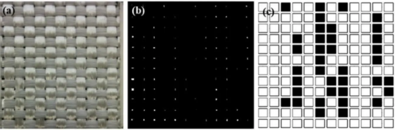
There are several reported causes for the stochastic variation in the permeability values of a fabric. Variation in the fabric architecture, handling of layers as they are placed over a tool surface, placement of the layers that nest to form the preform, and the manufacturing process all play a role [4,5]. Previous studies by Yun et al. found that there is an inherent randomness in through the thickness permeability of any woven fabric which can locally cause large variations in resin flow in through the thickness direction resulting in void formation [6]. The inherent variation in through the thickness permeability arises from the varying size of meso-scale spaces (pinholes) between woven tows. An example of an image of a woven fabric is presented inFig. 2(a). The raw picture of a woven fabric is given inFig. 2(a) and a filtered image using a proper threshold by MATLAB is presented inFig. 2(b). The pinholes of varying sizes act as easy pathways for resin from the DM to race through the thickness direction to reach the bottom layer of the stacked layers of fabrics. This results in uneven flow and possible merging of the flow fronts trapping the air which forms the voids [6]. The varying sizes and locations of the pinholes are statistically char-acterized with two statistical properties: a distribution function fit to the histogram of calculated permeability of pinholes (Kpin) and spatial
correlation of pinhole areas [7]. The method to calculated Kpin, , and
MI is well described in paper [6,7], andAppendix A. The distribution
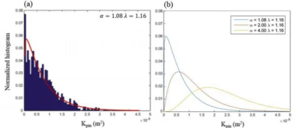
function best fit to the histogram is found to be gamma distribution and one of its parameter, the shape factor , has been explored to in-vestigate its effects on the overall Kpin. The example of the gamma
distribution fitting the histogram of pinhole permeability of the fabric presented inFig. 2is displayed inFig. 3(a) [7]. The gamma distribution shifts to the right as α increases from 1 to 4 as seen inFig. 3(b). Phy-sically this means that as that as α increases the average pinhole size increases and consequently Kpinvalues also increase. The spatial
cor-relation between pinhole areas and no pinhole areas is visually shown in Fig. 2(c) as a matrix composed of black (no pinhole) and white (pinhole) areas. Moran's I (MI) is a statistical measure of spatial cor-relation [8]. For this study, MI is used to study the spatial relationship between pinhole areas and no pinhole areas. The examples of varying MI are presented inFig. 4. The value of MI varies from 0 (no spatial correlation) to 0.5 (statistically significantly positively correlated). The range for these two important parameters of Kpinfield to describe the
fabric variability ( of 1–4 and MI of 0–0.5) should cover most of the woven fabrics. The mean radius of pinhole of as it increases from 1 to 4 increases from 0.7 mm to .1.7 mm. One will rarely encounter a woven fabric with pinhole size between two tows to be larger than 1.7 mm. For MI, one is hardly likely to encounter a woven fabric of MI over 0.5 as can be seen inFig. 4.
Numerical simulations were carried out to study the effects of MI
and on the flow pattern of resin and resulting void percentage.
Table 1shows the effect of these two parameters of fabric on the void percentage formed in a VARTM process. Liquid Injection Molding Si-mulation (LIMS) was utilized to run numerical siSi-mulations that describe Darcy's flow of resin into an anisotropic fabric in a 3D mold in which pinholes can be introduced in through the thickness direction. The implementation of pinhole permeability is well described in Ref. [7]. The pinhole location and size were selected by the value of and MI. Fig. 1. Schematic of the VARTM process to describe the impregnation of resin into the reinforcing woven fabric with high permeability distribution media placed on top of fabric layers to enhance the in-plane flow.
Fig. 2. Image of E-glass fabric (60 mm by 60 mm) (a), binary image (b), and pinhole matrix(c). Black indicates no pinhole area and white signifies presence of pinhole.
Note that although and MI value may be same, the distribution of pinholes and their correlation matrix can embody different patterns. The DM permeability can also be changed but was set to 1.4×10⁻⁸m2.
Mean percentage of voids by running 150 simulations for a given and MI was found to increase with increasing and MI. This is a predictable result because higher value of results in higher permeability of pin-holes and higher value of MI leads to more highly clustered pinhole spaces (positive correlation between pinhole areas).
Characterizing the fabric with these two parameters in real time can allow one to forecast the possible void percentage in a VARTM process for a given value of DM permeability. Machine learning methods are effective in achieving this goal of identifying a fabric with these two parameters quickly. Linear and non-linear dimensionality reduction methods are types of machine learning processes which visualize and characterize a group of high dimensional input data through a reduc-tion of dimensionality. Machine learning methods such as Principal Component Analysis (PCA), t – Distributed Stochastic Neighboring Embedding (t_SNE), and Locally Linear Embedding (LLE) are widely used to treat image, voice, and other types of samples with a high di-mension [9–19]. These techniques visualize and characterize a large number of samples with a high dimension in either two or three di-mensional space (map). In this study, the map refers to a 2D or 3D representation of high dimensional input data obtained through mani-fold learning techniques. The map is a useful co-relation tool as it helps one to identify which cluster the new sample will belong to in the map and this way the new sample can be classified accordingly. There are previously reported studies of dimensional reduction and data visuali-zation using LLE [13,18], PCA or kPCA [9,10,20], and SNE or t_SNE
method [11,14,19,21]. In this study, the objective is to identify two important parameters ( , MI) from a high dimensional input using di-mensionality reduction methods (PCA and t_SNE) to predict the void contents in a composite part by running numerical simulations.
2. Methodology
Two charts of the entire procedure which provides the void fraction range from an image of the fabric in real time is presented inFig. 5. The procedure consists of a training step and a testing step. For this study, a total of 450 samples for 9 cases (3 MIs of 0, 0.3, and 0.5 and 3 αs of 1, 2, and 4) are used as a training data set. The detailed procedure to create the training samples is well documented in Ref. [7]. In the training step, 450 images and matrices are first processed to generate frequency fil-tered version of input data by Fast Fourier transformation (FFT). The frequency matrices are further processed by PCA first to identify the
Fig. 3. Histogram of pinhole permeability of a plain woven fabric inFig. 2and its best fit gamma distribution function (a) and gamma distributions with varying α
(b).
Fig. 4. Samples of 21 × 21 mesh size and varying Moran's I. MI of 0 (a), 0.3 (b), and 0.5 (c and d representing two different realizations) Black indicates no pinhole area and white means pinhole area.
Table 1
Void percentage obtained from numerical simulation with varying and MI (MI). = 1 MI = 0 MI = 0.3= 1 MI = 0.5= 1 MI = 0.3= 2 MI = 0.3= 4 Range (%) 0.7–2.6 0.9–3.8 0.9–4.6 1.3–4.2 1.3–4.3 Mean (%) 1.35 1.90 2.05 2.30 2.54 Standard deviation (%) 0.37 0.65 0.75 0.47 0.50
important frequencies and ignore the others. Then, the more advanced t_SNE machine algorithm is applied to create 3D maps in which the input samples are separated based on α and MI. Once the maps in three dimensions show clear separation for these parameters, a binary image of a new sample of fabric is subjected to the machine learning methods in the testing step which will place it in a cluster of the created 3D map
thus identifying its and MI value. Once these two parameters are
known, the numerical simulations were performed with these values of α and MI for different DM permeability values. The corresponding range of void fractions can then be forecasted from the numerical si-mulations of the VARTM process from using just the binary image of the fabric sample.
2.1. Image processing
There are two types of image samples for the process. This binary image of size of 205 × 205 (dimensionality of 44100) pixels inFig. 2
(b) is one type of input data which is obtained by filtering the original image with a selected threshold. The binary image contains the in-formation of both the size and the location of the pinholes. The second input data is a pinhole matrix of size of 21 × 21 (dimensionality of 441) produced from the binary image as shown inFig. 2(c). Each cell of the matrix has information contained in 5 mm × 5 mm square of the binary image. The distance of 5 mm is the average distance between pinholes (tows) which lie horizontally or vertically. MATLAB is employed to import the images into binary matrix. The accuracy of the process of importing images is well documented in the paper [6,7]. The matrix elements are composed of 1 (no pinhole) and 0 (pinhole).
2.2. FFT and machine learning methods 2.2.1. Fast Fourier transformation (FFT)
In order to reduce the dimensionality and the noise within the do-main, the images and matrix of a woven fabric are transformed by FFT to output in a frequency domain using MATLAB [22]. FFT is a method to carry out Discrete Fourier Transformation (DFT) quickly and effi-ciently. DFT is a method that converts an input data in a spatial domain to output data with sine and cosine components in frequency domain. The elements in the binary image and pinhole matrix (X) are trans-formed to corresponding frequency ( ) by FFT. The output of FFT , is a matrix with each point displaying a particular frequency which is then addressed by the machine learning algorithm PCA followed by t_SNE.
2.2.2. Principal Component Analysis (PCA) and t – distributed Stochastic Neighbour Embedding (t_SNE)
PCA and t_SNE both are used to reduce the dimensionality of the processed matrix and images by FFT in this study. In PCA, the data in a principal sub-space is obtained using eigenvectors (principal compo-nents) of the covariance matrix of the input data [10,23]. t_SNE is a variation of SNE which is a nonlinear dimensionality reduction tech-nique by minimizing a cost function of probability distributions of neighboring points over the input data. It is easier to implement and yields much better visualization in a low dimensional space than standard SNE [14,21].
The procedure begins by subtracting mean from the processed fre-quency matrix, to obtain matrix, D1. Covariance matrix ( ) of D1 is calculated and eigenvalues and eigenvectors of the covariance matrix ( ) are obtained. K largest eigenvectors are then multiplied to the frequency matrix ( ) to obtain a matrix of reduced dimensionality ( 1) in PCA space [24,25]. In this study, K is 30 which means the initial dimensionality (44100 or 441) are reduced to 30 first eigen vectors using PCA method. The PCA treated matrix ( 1) is then processed by t_SNE to obtain a final matrix (y) of reduced dimension 3. First, the probabilities (p q, ) converted from euclidean distance between data points (in 1( 1 , 1 , , 1 )1 2 n1 for p and y (y y1, ,2 ,yn1) for q) are
presented (Equations(3) and (4)) [14]. = p exp exp( 1 1 /2 ) ( 1 1 /2 ) ij i j k l l k 2 2 2 2 (3) = q y y y y exp exp( ) ij i j k l k l 2 2 (4) Where the variance of the Gaussian is centered data point, 1iThese pairwise similarities (probabilities, p q, ) should be the same if the new map (y) models the similarities of input matrix ( 1) correctly. The cost function (C) in Equation(5)below measures the difference between two probabilities and it should be minimized to obtain the final matrix (y). =KL P Q = p log p q C ( ) i j ij ij ij (5)
The cost function, C, aims to minimize a single Kullback-Leibler divergence between p and q.
The early employment of PCA in the process helps to define the Fig. 5. Flow charts showing the process to obtain void fraction from an image of the fabric. Training step (a) and testing step (b).
main manifold from a linear dimensionality reduction perspective. It was found that FFT and PCA filters were necessary before employing t_SNE. MATLAB is employed to carry out the machine learning process implementation.
2.3. Numerical simulation (LIMS)
Numerical flow simulation with the generated random field where Kpin (permeability of a pinhole) values are assigned to through the
thickness permeability allows us to study the effect of heterogeneity on
the flow. LIMS is a finite element/control volume flow simulation software which was developed at the University of Delaware [26]. The woven fabric with pinholes inFig. 2was modeled into a 3D mesh with 1D elements representing the pinhole values for the simulation. The mesh is shown inFig. 6.
Four layers of fully nested fabrics (0.12 m by 0.53 m) and pinholes are simulated using 3D elements (representing the woven fabric) and 1D elements (representing the pinholes). The thickness of each layer of fabric is 0.7 mm under vacuum (fully nested). One layer of DM (0.11 m by 0.48 m) with thickness of 1 mm is simulated using 2D elements. The permeability tensor of the woven fabric was obtained experimentally using the methodology presented in Ref. [3]. The values of the bulk permeability components are presented inTable 2.
The Kpinfield was generated using the methodology documented in
Ref. [7] and was assigned to the 1D elements. Three values of DM permeability (KDM of 1.45×10 08 2m, 8.5×10 09 2m, and 4×10 09 2m)
were used to study the effect of KDMon void formation. Other
experi-mental conditions such as fabric volume fraction, pressure, and visc-osity are listed inTable 3.
The simulations were run to find the final void content. The void fraction was calculated as the area of the voids divided by the mold area. These numerical results along with the result from the machine learning method are used to provide the range of void content for any new image of the fabric.
3. Results
3.1. Results of manifold embedding method
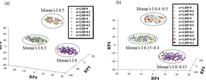
The results of manifold embedding of 450 images and matrices of varying α (1, 2, and 4) and MI (0, 0,3, and 0,5) are obtained and pre-sented inFigs. 7 and 8. A 3D map of clearly separated clusters based on was obtained using binary images of resolution of 205 × 205 pixels in the training step as can be seen inFig. 7. As briefly mentioned in In-troduction section, affects the size of pinholes. The higher the value of , it signifies on an average a larger size pinhole. Considering this, the result makes sense that images rather than matrices are proper training samples for the characterization of input data with in a reduced 3D space because the images show the size of pinholes. On the other hand, the second type of input data, matrices of 21 × 21 elements, only contains the information of the location of pinholes in a unit size of Fig. 6. Woven fabric layer modeled as 3D elements and pinholes as 1D elements
in the flow simulation [6]. Table 2
Experimentally determined permeability values of the components of the 3D permeability tensor of the plain woven fabric.
Kxx(m2) Kyy(m2) K mzz( 2) K mxz( 2) Kyz(m2) K mxz( 2)
8.8× 10 11 9.1× 10¹¹ 1.36× 10 12 9.89× 10¹⁶ 1.58× 10¹⁵ 1.00× 10 15
Table 3
Experimental condition for numerical simulation study.
Fabric volume fraction 0.45 Inlet Pressure (Pa) 1× 10⁵
Resin Viscosity (Pa.s) 0.1
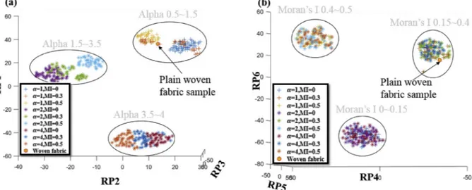
Fig. 7. Manifold embedding of input of images of fabric of 205 × 205 size in 3D space. Α separation of value of 1, 2 and 4 (a) and Α separation of value varying in range (0.5–4) (b). Here RP means reduced parameter.
fabric (105 mm by 105 mm) and of spatial correlation between pinholes and no pinhole areas. Therefore, matrices rather than images are chosen to be the training samples for characterization of data based on MI values and the results are presented inFig. 8. Additional samples of intermediate α of 0.5, 1.5, 2.5, and 3.5 were included in the training
pool along with samples of MI of 0.15 and 0.4.Figs. 7(a) and 8(a) show the result from manifold learning process with 9 samples (MI 0, 0.3 and 0.5. α of 1, 2, and 4). Figs. 7(b) and 8(b)show the results with all samples including the intermediate values of α and MI. is set to 1 for samples with varying MI, and MI is set to 0.3 for samples with varying Fig. 8. Manifold embedding of input matrix of 21 × 21 size in 3D space. MI separation of value of 0, 0.3, and 0.5 (a) and MI separation of value varying in range (0–0.5) (b). Here RP means reduced parameter.
Fig. 9. Plain woven fabric of size of 105 mm × 105 mm the width of tow is 5 mm original image (a) binary image (b) pinhole matrix (c). Black indicates no pinhole area and white indicates pinhole.
. These 3D maps can now be used to identify α and MI for a fabric of interest from its image as shown in the next section.
3.2. Experimental results
The plain woven fabric presented in Fig. 2was used as an input sample to identify its α and MI value using the method discussed in the previous section. The original image of size of 105 mm × 105 mm, binary image (205 × 205 pixels), and pinhole matrix (21 × 21 pixels) are displayed inFig. 9. The image and matrix data were processed by FFT first before subjecting it to the manifold embedding method. The position of the new sample in a 3D space is shown to belong to the cluster which has α in the range of 0.5–1.5 and MI in the range 0.15–0.4 inFig. 10. With this characterization of the fabric, one can forecast the expected void percentage range from the previously compiled library of numerical simulation results for various α and MI values. For α of 1 and MI of 0.3, the expected void fraction are presented in Table 4and
Fig. 11.
The numerical results show that the void fraction increases with higher DM permeability [3,7], and it could be up to 4.26% for this type of fabric with α of 1 and MI of 0.3.
4. Summary and conclusions
Manifold embedding method is successfully used to characterize the architecture of a fabric of interest with important variables such as α and MI. A total 450 training samples of varying α and MI were used for the manifold embedding method, PCA and t_SNE, to build a 3D map
showing distinctly separate clusters of input data separated based on the two variables (α and MI). To test the method, the manifold em-bedding method was carried out on an image of a new sample of a plain-woven fabric with tow width of 5 mm to identify the cluster of α and MI it belonged to in the 3D map of clusters created from the training samples. The α and MI were found to be in the range of 0.5–1.5 and 1.5–4, respectively for the fabric. The range of void fraction for this fabric was forecasted for the three DM cases to vary between 0.1 and 4%. This quick and efficient approach to characterize a fabric with two variables allows for forecasting the likelihood of void formation and its extend in the VARTM process and also provides textile manufacturers information on the effects of variability in their equipment on the manufacturing of the fabrics so steps could be taken to reduce this variability.
Fig. 10. Identification of the value of α (Fig. 10a) and MI (Fig. 10b) of the new woven fabric sample in the clustered manifold map built with 450 training samples
(seeFigs. 7 and 8) Here RP means reduced parameter.
Table 4
Void percentage obtained from numerical simulations performed with gener-ated pinhole positions and sizes for various α and MI values.
KDM(m2) Simulation results Void (%)
Range (%) Mean (%) Standard deviation 1.45× 10 08 1.06–4.26 1.90 0.56
8.5× 10 09 0.31–3.72 1.39 0.54
4× 10 09 0.12–3.33 0.79 0.47
Fig. 11. Histogram of void percentages calculated from the simulations with generated pinhole fields. Different colors represent different DM permeability magnitudes[7].(For interpretation of the references to color in this figure le-gend, the reader is referred to the Web version of this article.)
Appendix A
Moran's I index varies from −1 (negatively correlated) to 1 (positively correlated). = = = = = = = = = = = I n W W x x x x x x ( ¯)( ¯) ( ¯) i i n j j n ij i i n j j n ij i j i i n i 1 1 1 1 1 2 (A1)
WhereWijis the binary weight matrix,xiis the Kpinvalue at location i, xjis the Kpinvalue at location j, andx¯is the global mean of Kpin, values and n is
the total number of pinholes. In equation(A2),
= > +
f x( ) x e and x
( ) , , 0 0
X 1 x (A2)
Where x is the gamma random variable (in our case the Kpinvalue) and f xX( )is the gamma random variable density function, is a scale factor, and is a shape factor. The fitted gamma distribution of histogram of Kpinvalues is presented inFig. 3for which = 1.16 and = 1.08.
References
[1] W. H. Seemann, G. C. Tunis, A. P. Perrella, K. Rikard, E. H. Del, A. Everett, P.W.R.I, W. Schurgin, and H. Llp, “United States Patent 5,721,034,” 1998.
[2] X. Zeng, L.P. Brown, A. Endruweit, M. Matveev, A.C. Long, Geometrical modelling of 3D woven reinforcements for polymer composites: prediction of fabric perme-ability and composite mechanical properties, Compos. Part A Appl. Sci. Manuf. 56 (2014) 150–160.
[3] M. Yun, H. Sas, P. Simacek, S.G. Advani, Characterization of 3D fabric permeability with skew terms, Compos. Part A Appl. Sci. Manuf. (December 2016) 2017. [4] R. Arbter, J.M. Beraud, C. Binetruy, L. Bizet, J. Breard, S. Comas-Cardona,
C. Demaria, A. Endruweit, P. Ermanni, F. Gommer, S. Hasanovic, P. Henrat, F. Klunker, B. Laine, S. Lavanchy, S.V. Lomov, A. Long, V. Michaud, G. Morren, E. Ruiz, H. Sol, F. Trochu, B. Verleye, M. Wietgrefe, W. Wu, G. Ziegmann, Experimental determination of the permeability of textiles: a benchmark exercise, Compos. Part A Appl. Sci. Manuf. 42 (9) (2011) 1157–1168.
[5] N. Vernet, E. Ruiz, S. Advani, J.B. Alms, M. Aubert, M. Barburski, B. Barari, J.M. Beraud, D.C. Berg, N. Correia, M. Danzi, T. Delavière, M. Dickert, C. Di Fratta, A. Endruweit, P. Ermanni, G. Francucci, J.A. Garcia, A. George, C. Hahn, F. Klunker, S.V. Lomov, A. Long, B. Louis, J. Maldonado, R. Meier, V. Michaud, H. Perrin, K. Pillai, E. Rodriguez, F. Trochu, S. Verheyden, M. Weitgrefe, W. Xiong, S. Zaremba, G. Ziegmann, Experimental determination of the permeability of en-gineering textiles: benchmark II, Compos. Part A Appl. Sci. Manuf. 61 (2014) 172–184.
[6] M. Yun, T. Carella, P. Simacek, S. Advani, Stochastic modeling of through the thickness permeability variation in a fabric and its effect on void formation during Vacuum Assisted Resin Transfer Molding, Compos. Sci. Technol. 149 (2017) 100–107.
[7] M. Yun, P. Simacek, C. Binetruy, S. Advani, Random field generation of stochasti-cally varying through the thickness permeability of a plain woven fabric, Compos. Sci. Technol. 159 (2018) 199–207.
[8] C. Zhang, L. Luo, W. Xu, V. Ledwith, Use of local Moran's I and GIS to identify pollution hotspots of Pb in urban soils of Galway, Ireland, 8 (2008). [9] J.C. Isaacs, S.Y. Foo, A. Meyer-Baese, Novel kernels and kernel PCA for pattern
recognition, Proc. 2007 IEEE Int. Symp. Comput. Intell. Robot. Autom. CIRA 2007, 2007, pp. 438–443.
[10] Q. Wang, Kernel principal component Analysis and its applications in face
recognition and active shape models,arxiv:1207.3538, (2012).
[11] A. Gisbrecht, A. Schulz, B. Hammer, Parametric nonlinear dimensionality reduction using kernel t-SNE, Neurocomputing 147 (1) (2015) 71–82.
[12] L.K.L. Saul, S.S.T. Roweis, Think globally, fit locally: unsupervised learning of low dimensional manifolds, J. Mach. Learn. Res. 4 (1999) (2003) 119–155. [13] E. Lopez, D. Gonzalez, J. V Aguado, E. Cueto, C. Binetruy, F. Chinesta, A manifold
learning approach for integrated computational materials engineering, 25 (1) (2018) 59–68.
[14] L.J.P. Van Der Maaten, G.E. Hinton, Visualizing high-dimensional data using t-sne, J. Mach. Learn. Res. 9 (2008) 2579–2605.
[15] S.T. Roweis, Nonlinear dimensionality reduction by locally linear embedding, 2323 (2000) (2009).
[16] S. Wold, K.I.M. Esbensen, P. Geladi, Principal component Analysis, SpringerReference 2 (1987) 37–52.
[17] G. Guo, Y. Fu, C.R. Dyer, T.S. Huang, Image-based human age estimation by manifold learning and locally adjusted robust regression, IEEE Trans. Image Process. 17 (7) (2008) 1178–1188.
[18] E. Lopez, E. Abisset-Chavanne, F. Lebel, R. Upadhyay, S. Comas, C. Binetruy, F. Chinesta, Advanced thermal simulation of processes involving materials ex-hibiting fine-scale microstructures, Int. J. Mater. Form. 9 (2) (2016) 179–202. [19] A.R. Jamieson, M.L. Giger, K. Drukker, H. Li, Y. Yuan, N. Bhooshan, Exploring
nonlinear feature space dimension reduction and data representation in breast CADx with Laplacian eigenmaps and t -SNE, Med. Phys. 37 (1) (2010) 339–351. [20] A.N. Kandpal, B.B.M. Rao, Implementation of PCA & ICA for voice ecognition and
separation of speech, ICAMS 2010 - Proc. 2010 IEEE Int. Conf. Adv. Manag. Sci. vol. 3, 2010, pp. 536–538.
[21] G. Hinton, S. Roweis, Stochastic Neighbor Embedding, (2002).
[22] F.C. Elena Lopez, Adrien Scheuer, Emmanuelle Abisset-Chavanne, On the effect of phase transition on the manifold dimensionality: application to the Ising model, Math. Mech. Complex Syst. 6 (3) (2018).
[23] C.M. Bishop, Pattern Recognition and Machine Learning, 53 (9) (2013). [24] H.J. Kim, K.I.a Jung, K.b Kim, Face recognition using kernel principal component
Analysis, IEEE Signal Process. Lett. 9 (2) (2002) 40–42.
[25] V. Scienzia, S.E. Non, P. Per, L.D.A. Vinci, Mathematics and Mechanics of Complex Systems, 6 (3) (2018).
[26] P. Šimáček, S.G. Advani, Desirable features in mold filling simulations for liquid composite molding processes, Polym. Compos. 25 (4) (2004) 355–367.