An Application of Deep Reinforcement Learning to Algorithmic Trading
Texte intégral
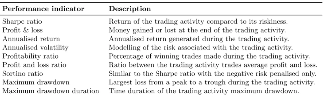
Figure

Documents relatifs
Distribution and Abundance of Resting Cysts of the Toxic Dinoflagellates Alexandrium tamarense and 751. catenella in sediments of the eastern Seto Inland Sea, Japan,
De plus, comme cela a été évoqué dans la section précédente, cette méthode de pré- diction de l'intervalle RR pourrait servir à l'attribution du signal de phase cardiaque
In addition, we use the most general (and powerful) server assignment policy, where the requests of a client can be served by multiple servers located in the (unique) path from
Zhou, F., Zhou, H., Yang, Z., Yang, L.: EMD2FNN: A strategy combining empirical mode decomposition and factorization machine based neural network for stock market
Volume, relative strength index, price-to-earnings ratio, moving av- erage prices from technical analysis, and the conditional volatility from a GARCH model are considered as
We tested Deep reinforcement learning for the optimal non-linear control of a chaotic system [1], using an actor-critic algorithm, the Deep Deterministic
Pham Tran Anh Quang, Yassine Hadjadj-Aoul, and Abdelkader Outtagarts : “A deep reinforcement learning approach for VNF Forwarding Graph Embedding”. In IEEE, Transactions on Network
To overcome these issues, we combine, in this work, deep reinforcement learning and relational graph convolutional neural networks in order to automatically learn how to improve
