A TWO-TIME SCALE SIMULATION FOR DYNAMIC ANALYSIS OF POWER SYSTEMS
R. Ramirez-Betancoura, C.R. Fuerte-Esquivela,*, T. Van Cutsemb
a Universidad Michoacana de San Nicolás de Hidalgo, Faculty of Electrical Enginering, Morelia, Michoacán, México. b FNRS and University of Liège, Department of Electrical Engineering and Computer Science of the, Sart Tilman B37,
B-4000 Liège, Belgium.
*
Corresponding author. Tel.: +52 443 3 27 97 28; fax: +52 443 3 27 97 28 E-mail address: cfuerte@umich .mx
Abstract
This paper proposes a two-time scale simulation approach of both short-term and long-term dynamics in power systems. The short-term transient period is analyzed by a full-time scale simulation while a quasi-steady state model of the power system is used to simulate long-term dynamics. The proposed method is inspired of Singular Perturbation theory to model the interaction between the short-term and long-term dynamics. Based on this interaction, a suitable criterion to determine when the quasi-steady state model of a power system can be considered as a uniform approximation of the full-time scale model is proposed, which also determines the appropriate switching time between models. The proposed method is demonstrated on the 10-machine, 39-bus New England system and a 46-machine, 190-bus equivalent Mexican system.
Keywords: Long-term dynamics, quasi-steady state approximation, singular perturbation theory, time scale decomposition.
1. Introduction
Generally speaking, modern power systems are large-scale systems composed by the interconnection of electric components whose dynamics are interacting at widely-varying speeds [1]. Following a disturbance which does not cause short-term instability, the so-called long-term dynamics can persist over several minutes (and even more in some cases). Consequently, long-term dynamic simulations must be carried out considering both fast and slow dynamics of the system to accurately analyze the effects of large excursions of voltage, frequency, and power flows that may invoke
the action of slow processes, controls and protections. This analysis requires the step-by-step numerical integration of a large-scale nonlinear stiff set of differential-algebraic equations (DAEs). As a consequence, long-term simulations require very large computational efforts if appropriate techniques are not used.
There are two main approaches to using time scales to reduce the computational burden of long-term dynamic simulations: i) full time scale (FTS) simulation technique using a variable time step size of integration in conjunction with explicit or implicit integration methods [2]-[6]; ii) model reduction-simplification techniques in conjunction with implicit integration methods [1], [7]-[11].
Approaches that automatically adjust the time step of integration in accordance with the system’s dominant transients are used to study both short and long-term dynamic phenomena in integrated simulation tools [2]-[4]. The main idea behind these approaches is to automatically reduce the time step to capture fast transients. As fast modes decay during the solutions process, the time step is gradually increased to reduce the computation time required to capture slow transients. The time step size (and possibly the order) of the integration method are adjusted, usually according to a truncation error defined as the difference between predicted and corrected solutions [2], [4], or the weighted root square mean norm of all corrected values of dynamic and algebraic variables [3]. The integration steps have to be further adjusted in order to fall on the time instants where discrete state events (such as variables hitting their limits) take place. In case where the long-term dynamics are driven by many discrete controls – such as the widely used Load Tap Changers (LTCs) – this may prevent the step size from being increased to the extent allowed by the slow continuous-time dynamics.
Alternatively, the multiple time scales inherent to the dynamics of a power system can be exploited to obtain reduced order models relevant to a particular time scale [1], [12], [13] with the objective of simulating those reduced models much more efficiently [13], [14].
A first step toward model simplification was proposed in [5] with a unified approach to short and long-term dynamic simulation using fixed-step trapezoidal integration. The simulation mode is determined by the integration step size, and the switching from one mode to the other is defined by the degree of damping of synchronizing oscillations. An artificial damping term is included in the rotor swing equations of each generator to allow synchronizing oscillations to be artificially suppressed, and to allow larger integration time step when simulating the long-term mode.
More recently a decoupled time-domain based on invariant subspace partition and fixed step integration simulation was proposed in [6]. The original set of nonlinear Ordinary Differential Equations (ODEs) are grouped in two decoupled sets of stiff and non-stiff equations, respectively, based on eigenvalue analysis of the linearized set of ODEs.
The set of stiff ODEs, together with the set of algebraic equations, are solved using the trapezoidal integration method, while the forward Euler method is used to solve the rest of non-stiff ODEs.
Opposite to the approaches [2]-[6] where the original set of ODEs is handled throughout the whole simulation, the Quasi-Steady State (QSS) approximation of the long-term dynamics handles a reduced and simplified set of equations [1], [7], [13].
The QSS approach was devised in the context of dynamic security assessment where the response to an initial disturbance is studied until either the system returns to steady-state operation or some variables take values outside an acceptable range (for instance, voltages become unacceptably low in the case of long-term voltage instability, a problem for which the QSS technique has been extensively used). The analysis of real-life scenarios reveals the following characteristic behavior, common to almost all power systems. Over a period of up to – say - 20 s after the initiating disturbance, the system response is dominated by the short-term dynamics of the synchronous generators and their regulators, induction motors, static var compensators and STATCOMs, HVDC links and other power electronics-based devices. One possible outcome is a short-term instability that may take on the form of angular instability (loss of synchronism), frequency instability or short-term voltage instability. If the system responds in a stable way, it enters the long-term period where it is driven by slower phenomena, controllers and protections such as: load tap changers, field current limiters, automatic shunt compensation switching, secondary frequency and voltage controls, load power restoration, etc. The system may also evolve towards instability over this time interval of – typically – several minutes, for instance due to long-term voltage instability. Over the short-term period, the various synchronous generators oscillate with respect to each other while during the long-term interval, in most cases, those inter-machine oscillations are negligible and the common speed of all machines defines the system angular frequency. One cannot exclude, however, a badly damped slow, interarea mode to show its effect over a time interval that exceeds the above cited short-term period; there is no clear-cut border between the short and long-short-term intervals.
The QSS approximation of long-term dynamics is obtained by considering a time-scale decomposition of the dynamic state variables into fast and slow time-varying variables, respectively, and assuming that the former set of variables changes instantaneously with respect to variations of slow state variables, replacing the corresponding differential equations by their equilibrium conditions.
Although this approach tremendously reduces the computational burden for long-term dynamic simulations, it has the following limitations [8], [9]: i) it assumes stable short-term dynamics, while the system may lose stability in this time interval and hence not enter in the long-term period; ii) a large disturbance may trigger controls associated with
discrete events in the short-term period, and that sequence of fast controls may not be correctly identified from the QSS model.
These limitations can be overcome by using the FTS simulation to analyze the short-term time period and then switching to the QSS approximation to compute the long-term dynamics. In [8], the switching from FTS to QSS simulation is done once the frequency changes are below a specified value. At the switching time tsw, the QSS model is
initialized from the last system’s short-term state and is used for the rest of the simulation neglecting frequency dynamics. On the other hand, a different coupling of both approaches, based on the discrete events taking place during the detailed simulation was proposed in [9]. The FTS simulation is executed until the switching time tsw and the
sequence of discrete events that have occurred over this interval is identified. The QSS simulation is then performed from the initial time with those discrete events imposed as external disturbances, without allowing the discrete devices to act by themselves until the simulation time arrives at tsw. From there on, the study proceeds with the usual QSS
approximation.
Following the idea of combining FTS and QSS models, this paper proposes a two-time scale simulation approach for a unified solution of both fast and slow dynamics. The proposed method is inspired of Singular Perturbation theory to model the interaction between short and long-term dynamics [10], [11]. Based on this interaction, a suitable criterion is proposed to accurately determine when the QSS model of a power system can be considered as a uniform approximation of the FTS model, which also determines the appropriate switching time between these models. The main contributions of the proposed approach are the following: i) simulation efficiency is achieved by both time step size adjustment and model reduction, which are implemented in a single simulation tool instead of using only the former [2]-[5] or only the latter [7]; ii) the proposed criterion to automatically switch from the FTS to QSS models preserves a uniform approximation of state and algebraic variables, such that a process to initialize variables for the QSS simulation is not necessary; iii) finally, the proposed switching criterion is easily computed from the FTS simulation by monitoring the rate of change of the fast time-varying state variables.
2. Statement of the problem
2.1 Singular perturbations and two-time scales
Power system dynamics can be described by a mixed set of parameter-dependent differential and algebraic equations (DAEs), as given by the FTS model (1)
[
0]
( , , ) : 0 ( , , ) : ( ) ( , , ( )) : , n m p n n m p m n m p p k k n m p end x f x y z f g x y z g z t h x y z t h x X y Y z Z t t t + + + + + − + + = ℜ → ℜ = ℜ → ℜ = ℜ → ℜ ∈ ⊂ ℜ ∈ ⊂ ℜ ∈ ⊂ ℜ ∈ & (1)where t0 and tend are the initial and final times, respectively, of the study time period. x is a n-dimensional vector of
dynamic state variables with initial conditions x t( )0 =x0, y is a m-dimensional vector of instantaneous state (algebraic) variables, (usually the real and imaginary parts or the magnitudes and phase angles of the complex node voltages) with initial conditions y t( )0 =y0, and z is a set of p discrete states which undergoes step changes from z t( )k− to z t( )k+ at some instant tk [13]. Because transmission network dynamics are much faster than dynamics of the equipment or loads, the
variables y are understood to change instantaneously with variations of the x states under the quasi-sinusoidal (or phasor) approximation. Hence, only the dynamics of the equipment, e.g. generators, controls, and loads at buses, are explicitly modeled by the set of nonlinear ordinary differential equationsx&= ⋅f( ). The set of nonlinear algebraic equations 0= ⋅g( ) represents the stator algebraic equations and mismatch power flow equations at each node. Lastly, the set of discrete-time equations z t( )k+ = ⋅h( )capture the discrete controls and protections acting on the system.
The set of differential equations x&= ⋅f( ) can be partitioned according to the time scales of the state dynamics. In particular, in a two-time scale system, (1) can be expressed as a standard form of the singular perturbation problem [11],
[
0]
( , , , ) : ( , , , ) : 0 ( , , , ) : ( ) ( , , , ( )) : , sd sd fd fd sd fd sd fd fd sd n m p n sd sd sd fd sd n m p n fd fd sd fd fd n n m p m sd fd n n m p p k sd fd k n n sd fd end x f x x y z f x f x x y z f g x x y z g z t h x x y z t h x X x X t t t ε + + + + + + + + + + + − = ℜ → ℜ = ℜ → ℜ = ℜ → ℜ = ℜ → ℜ ∈ ⊂ ℜ ∈ ⊂ ℜ ∈ & & (2)where xsd is a nsd-dimensional vector with predominantly slow dynamics, and initial conditions xsd( )t0 =xsd0 , while xfd is
a nfd-dimensional vector of states that have fast dynamics superimposed on slow varying quasi-steady state responses
with initial conditions 0 0
( )
fd fd
x
t
=
x
. When functions fsd( )⋅ and ffd( )⋅ are scaled to have the same order of magnitude, the perturbation parameter ε represents the ratio of time scales associated with xsd and xfd: ratios of small and large timeOne simple technique to reduce the order of the model (2), thereby reducing the stiffness of the system, is to formally set ε=0. In this case, dynamics of xfd become infinitely faster than xsd and instantaneously reach their
equilibrium ffd(·)=0, such that the system approaches the solution of the nsd-dimensional slow-reduced or QSS model (3)
if the Jacobian ∂ffd( )⋅ ∂xfdis nonsingular [11],
( , , , ) 0 ( , , , ) 0 ( , , , ) ( ) ( , , , ( )) sm sm sm sd sd sd fd sm sm fd sd fd sm sm sd fd sm sm k sd fd k x f x x y z f x x y z g x x y z z t+ h x x y z t− = = = = & (3)
In this case, the solution sm( )
sd
x t represents an approximation to the actual slow subsystem dynamics xsd( )t , and ( )
sm fd
x t represents an approximation of the slow modes (hence the upperscript sm) of the fast subsystem dynamics xfd( )t . This approximation is accurate for t∈
[
tsw,tend]
, where tsw is the time instant at which it is appropriate to switch frommodel (2) to model (3) . The values of algebraic variables associated with the slow dynamics are represented by y . The discrepancy between the responses computed from the QSS model (3) and from the FTS model (1) is due to the fast dynamic response. However, the equivalence between both responses can be established by investigating the dynamics of the fast-reduced model, which can be derived from (2) by considering the fast time scale τ , and the fast modes xsdfm( )τ and ( ) fm fd x τ , such that [11]: , sd( ) sdsm( ) sdfm( ), fd( ) smfd( ) fdfm( ) t x t x t x x t x t x τ τ τ ε = = + = + (4)
The fast reduced model (5) is then obtained by substituting (4) into (2), applying the chain rule, and letting ε→0
0 ( , , , ) 0 ( , , , ) ( ) ( , , , ( )) fm sd fm fd sm sm fm fd sd fd fd sm sm fm sd fd fd sm sm fm k sd fd fd k dx d dx f x x x y z d g x x x y z z t h x x x y z t τ τ + − = = + = + = + (5)
The first equation of (5) implies that xsdfm is frozen at its initial value xsdfm( )t0 . Furthermore, as xsd is predominantly
slow, we can constrain the quasi-steady state xsdsm to start from the prescribed initial condition xsdsm( )t0 =xsd( )t0 =xsd0 , which implies that fm( )0 0
sd
x t = . Based on this assumption, the approximation of xsd by xsdsmis uniform for all t∈[t0, tend]
with errors on the order of ε, i.e. sm ( )
sd sd
x =x +Oε , and fm( ) 0
sd
x τ = for all τ∈[t0, tsw] [11], [15].
The fast modes xfmfd of xfd are the states of the fast reduced model (5) which will damp out to their equilibrium
( ) 0
fm
fd sw
x τ =t = if they are asymptotically stable. In this case, a uniform approximation of the fast dynamics is given by
( )
sm fm
fd fd fd
x =x +x +O ε over t∈[t0, tsw], and once the fast modes become small enough, xsmfd( )t is a uniform approximation
of xfd(t), xfd =xsmfd +O( )ε , for t∈[tsw, tend].
Based on the theory described above, the Tikhonov’s theorem [15] guarantees that the solution given by the QSS model (3) uniformly approximates the true solution computed from (1) after a time interval t∈[t0, tsw] has elapsed.
Hence, our proposal to tackle the complexity of dynamic long-term simulations consists of using the FTS model (1) to simulate the dynamics associated with the short-time period following a disturbance with a small step size, and once the fast dynamics are small enough, switching to the slow-reduced model (3) to perform the long-term simulation with a larger step size. Owing to the fact that at the switching time there exists a uniform approximation between models, the state and algebraic variables of the slow reduced model are automatically initialized from the final system state provided by the full simulation. Lastly, the information required to determine the evolution of the discrete states z is directly transferred from the FTS simulation to the QSS model.
2.2 Switching criterion
An appropriate criterion to determine when the fast modes fm fd
x are small enough, which is the necessary condition to switch from the FTS model to the QSS model, can be determined using the singular perturbation technique as detailed hereafter.
The sets of ODEs in (2) associated with the dynamic models of power system components can be represented in their linearized form, such that the singular perturbation model can be reformulated by considering fm 0
sd
(
)
(
)
21 22 23 2 11 12 13 1 0 ( , , , ) ( ) ( , , , ( )) sm fm sm sd fd fd sd sm fm sm fd fd fd sd sm sm fm sd fd fd sm sm fm k sd fd fd k x A x x A x A y B u x A x x A x A y B u g x x x y z z t h x x x y z t ε + − = + + + + = + + + + = + = + & & (6)where Aij are constant matrices of appropriate dimensions. Similarity, the QSS model (3) consists of neglecting fm
fd
x while setting ε=0, which yields:
21 22 23 2 11 12 13 1 0 0 ( , , , ) ( ) ( , , , ( )) sm sm sm sd fd sd sm sm fd sd sm sm sd fd sm sm k sd fd k x A x A x A y B u A x A x A y B u g x x y z z t+ h x x y z t− = + + + = + + + = = & (7)
The second equation of (7) can be solved for sm fd
x , and the resulting expression can be substituted into the second equation of (6) to obtain (8) that permits the computation of the fast modes
(
)
(
)
1 11 13 fm fd fd x =A− εx& −A y−y (8)Since the change of xfd will lag far behind the instantaneous change of algebraic variables, and considering that the
difference
(
y−y)
tends to zero faster thanx
&
fd , as numerically shown in § 2.4, one can assume that a good approximation to compute xfdfm can be obtained by1 11 fm
fd fd
x =A−εx& (9)
where x& is computed by the integration of the full model at each time step. Therefore, (9) can be evaluated without fd
additional computational cost. Since the dynamics of fm
fd
x are associated with different fast state variables, the normalized value of each
1, , fm fd i nor fd i fd fd i x x i n x = = … (10)
Therefore, the time of switching t from the full model to the slow reduced model is determined when the maximum sw
absolute value of xnorfd isalways smaller than a specified tolerance Tolsw, max xnorfd ≤Tolsw, for the whole pre-specified
period of time tTOL or its equivalent number of time steps tTOL/h.
2.3 Proposed long-term dynamic simulation
The proposed procedure for long-term dynamic analysis using the switching criterion is as follows.
Step 1.-For a given initial disturbance, select the fast and slow-state variables, x=(xfd , xsd), to ensure that the system
is state separable.
Step 2.-Solve the full model (1) with a small time step of integration, and check the switching criterion. For instance, the trapezoidal rule can be applied to algebraize the differential equations, such that the set of DAEs are expressed as a set of algebraic-difference equations
( )
1(
1)
1 0 2 k k h k k F ⋅ =x + −x − f + + f = (11)( )
1 2 0 k F ⋅ =g + = (12)where h is the integration time step, and the superscript k is an index for the time instant tk at which variables and
functions are evaluated: xk =x t
( )
k and fk = f x(
k,yk)
. The Newton-Raphson (NR) algorithm is used to solve (11, 12), where at the i-th iteration the following linear system is solved( )
( )
1 1 1 1 1 2 2 2 i i i k k k x y k k k x y h h I f f x F F y g g + + + + − − ∆ ⋅ = − ∆ ⋅ (13)For given valuesxk ykT
, the method starts from an initial guess 0 1 0 1
T
k k k k
x + x y + y
= =
and updates the
possible short-term instability associated with loss of synchronism or voltage instability is checked, and if it takes place, the simulation stops. The switching criterion is also checked at each time instant tk to determine the switching time.
When this criterion is satisfied continuously during tTol as indicated in
§ 2.2
, the algorithm proceeds with Step 3; otherwise, Step 2 is repeated.Step 3.-The simulation switches to the QSS model (3), which is solved as explained in Step 2 with a larger time
step of integration. At the switching time, initial conditions of QSS variables sm, sm,
sd fd
x x and y are set to values
, , sw sw t t sd fd x x andytsw respectively. 2.4 Application example
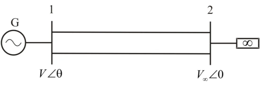
In this section the well-known one-machine infinite-bus system is used to illustrate the application of the proposed methodology. The system is shown with single-line diagram in Figure 1. The system data are given in Appendix A.
The generator is represented by a two-axis model with the following set of equations [16]:
(
)
1 2 1 3 cos do q q d fd T' E'& =K E' +Kψ +K V δ θ− +E (14)(
)
1 4 5 1 6 cos do d q d T'' ψ& =K E' +Kψ +K V δ θ− (15)(
)
1 7 1 8 2 9 sin qo q q q T' ψ& =Kψ +Kψ +K V δ θ− (16)(
)
2 10 1 11 2 12 sin qo q q q T'' ψ& =K ψ +K ψ +K V δ θ− (17) s δ ω ω&= − (18)(
)
2 s g m s P P D H ω ω&= − − ω ω− (19)where Ki are constants, E is excitation voltage (assumed constant in this example), H is the inertia constant, D is the fd damping constant, Pg is the generator’s electrical power output, Pm is the turbine mechanical power, δ is the
generator’s rotor angle in radians, ωs is the synchronous speed, and ω is the actual rotor speed. E' is the e.m.f. behind q transient reactance. Flux linkages of rotor windings along direct and quadrature axes are given by ψ1d, ψ1q andψ2q.
,
do do
T' T'' and T'qo,T'' are the time constants associated with the d-axis and the q-axis windings, respectively. Lastly, qo V and θ are the magnitude and phase angle of the voltage at bus 1.
The network equations are written in terms of active and reactive power mismatch equations [13],
( )
( )
(
)
2 11 1 1 0=Pg −V G +VV∞ G∞cos θ +B∞sin θ (20)( )
( )
(
)
2 11 1 1 0=Qg −V B +VV∞ G∞sin θ −B∞cos θ (21)where
(
)
(
)
(
)
(
)
(
)
(
)
13 1 14 2 15 16 1 2 17cos cos sin sin
sin 2 g q q q d P K V K V K E' V K V K V ψ δ θ ψ δ θ δ θ ψ δ θ δ θ = − − − + − + − + − (22)
(
)
(
)
(
)
(
)
(
)
(
)
(
)
13 1 14 2 15 16 1 2 2 2 3 6sin sin cos cos
cos sin g q q q d Q K V K V K E' V K V V C C ψ δ θ ψ δ θ δ θ ψ δ θ δ θ δ θ = − − + − + − + − − − + − (23)
The time constants T''do,T'qo, and T'' are generally small. Hence,qo ψ1d, ψ1q and ψ2q can be considered fast-time
varying variables, while E'q,δ and ωcan be assumed to be slow-time varying variables. Therefore, the FTS model has the following state vectors:
[
]
T y= θ V (24) 1 1 2 T sm fm fd fd fd d q q x =x +x =ψ ψ ψ (25) T sd q x =E' δ ω (26)while the slow-reduced model is represented by
T y=θ V (27) 1 1 2 T sm sm sm sm fd d q q x =ψ ψ ψ (28) T sm sd q x =E' δ ω (29)
The proposed switching criterion relies on computing xnorfd given by 1 2 1 5 7 11 1 1 2 T q q nor d fd do qo qo d q q x K T'' ψ K T' ψ K T'' ψ ψ ψ ψ = & & & (30)
such that the switching time is obtained when the condition max nor
fd sw
x ≤Tol has been satisfied continuously for a
pre-specified fixed number of time steps tTol.
In order to numerically validate the proposed switching criterion, a single contingency scenario is defined by removing one transmission line at time t=1s. Following the disturbance, an FTS simulation and a QSS simulation are performed with an integration time step of h=0.01s. Figure 2 shows the evolution of the voltage magnitude V and flux linkage ψ1q as a function of time computed by both simulations. When the disturbance takes place, the equivalent impedance between buses 1 and 2 increases, causing the voltage magnitude at bus 1 to also increase (over such a short period of time the machine behaves as a constant emf behind subtransient reactance). After the disturbance, the dynamic evolution of these two state variables depends on the simulation method. Since the voltage magnitude is an algebraic variable in both the FTS and the QSS simulations, its change is instantaneous. In the FTS simulation, the flux linkage evolves due to short-term electromagnetic transients. In the QSS simulation, on the other hand, the latter are neglected and the flux linkage becomes an algebraic variable which can thus change instantaneously. In the following instants of the QSS simulation, the flux evolves under the effect of the variables whose dynamics are not neglected. Nevertheless, the QSS response of this variable is quite acceptable once the fast dynamics have been damped out.
A comparison of these evolutions shows that the existing difference of the algebraic variable’s value V computed by both FTS and QSS simulations, V−V , is much smaller than the difference between the values of the fast-state
variable ψ1q, 1 1sm
q q
ψ ψ
−
, computed by each simulation. Therefore, the proposed criterion can be considered a suitable
method to determine the switching time. The system survives the short-term period, and the switching criterion is satisfied at t=2.2s with TOLsw=0.1 and tTOL=0.1s. At this time tsw, the values of state and algebraic variables computed
by FTS and QSS simulations are very close to each other, indicating that fast dynamics have died out and long-term responses can be assessed by the simpler QSS model.
The suitability of the proposed approach to analyze short- and long-term dynamics is tested on the 10-machine, 39-bus New England system and the 49-machine, 190-39-bus model of the Mexican power system. The design of the study cases is given below. All simulations were run on a laptop computer with the following characteristics: Intel processor dual core at 1.728 GHz, total RAM Memory of 2.00 GB, and operating system Windows XP.
3.1 10- Machine, 39-Bus New England System
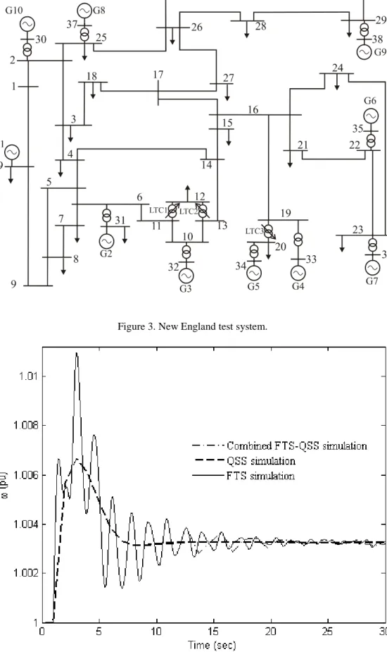
For the purpose of this test case, the generators were selected to be steam power plants. Generating plants were assumed to be equipped with an exciter, an automatic voltage regulator, a speed governor and a steam turbine. All exciters include derivative feedback compensation [17]. The data of this system were taken from [16], however gains and time constants were adjusted to make rotor oscillations last longer. Likewise, three Load Tap Changers (LTC) were installed on transformers to keep the voltage magnitudes at buses 12 and 20 at 1 p.u. with a half-deadband of ± 0.01 pu, as shown in Figure 3. All loads are represented with the exponential model [13]. For the specified disturbance, long-term dynamics come from the LTCs’ control actions [13] whose data are given in Appendix B. In this case, the LTC’s delay is 20 seconds on the first tap change and 10 seconds on subsequent tap changes, resulting each in a 0.01 pu change of the ratios. Additionally, steam turbines and governors act in the long-term to avoid large excursions of frequency.
At time t=1s, the system is suddenly perturbed by completely disconnecting the loads at buses 4, 20 and 29. A long-term simulation is performed with the full model, the combined FTS-QSS model, and the QSS model, respectively. The FTS simulation assumes that each generator has its own frequency of oscillation. On the other hand, a perfect coherency between all generators is assumed in the QSS simulations [7]. This assumption is valid in the long-term period as shown when comparing the responses provided by FTS and FTS-QSS simulations. Integration step sizes are defined according to the model being used in the analysis: the FTS model is integrated using a time step of 0.01s, while the QSS simulation is accomplished with an integration time step of 1s. Hence, the combined FTS-QSS simulation allows increasing the step size from 0.01s to 1s at the switching time. The fast-state variables monitored to carry out the switching from the FTS to QSS model are those associated with the exciters (Efd), generators (ψ1d, ψ1q,
ψ2q), and turbines (Plp, Php). Considering a switching tolerance of 0.1 and tTOL=0.1s, the fast variables of exciters,
generators, and turbines satisfy the switching criterion at 1.61s, 12.3s, and 12.67s, respectively, such that the switching of models takes place at t=12.67s.
dynamics. Figure 4 shows the rotor speed associated with the most critical generator, which is connected at node 34. Note that all the simulations tend to the same equilibrium point after the fast dynamics have been damped out. This demonstrates the suitability of the switching criterion in the sense that the switching between models is done once the short-term dynamics are small enough, as shown in Figure 5 for the field voltage Efd behavior of the generator at bus 34.
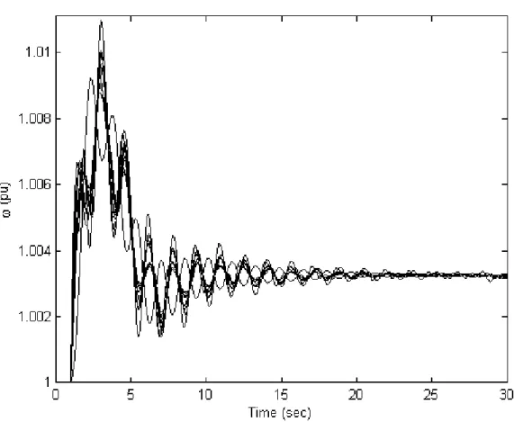
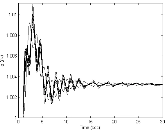
The evolution of the angular speed of all generators computed by the FTS, FTS-QSS and QSS simulations are shown in Figures 6, 7 and 8, respectively. Although the former two simulations are performed with each generator having its own rotor speed, while perfect coherency is assumed for the latter simulation, the same steady-state value of frequency is arrived at.
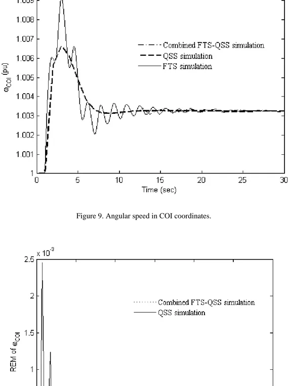
The angular speed ωCOI of the Center of Inertia (COI) is shown in Figure 9. As expected, the frequency transient behavior computed by the QSS model quickly tends to the equilibrium value reached by the other two models. Figure 10 shows the Relative Error Magnitude (REM) between the results obtained by the FTS-QSS and QSS simulations with respect to that obtained by the FTS simulation. As it is expected, the error of ωCOI associated with the proposed
approach is null during the short-time period and amounts to very small values after the switching time tsw=12.67s.
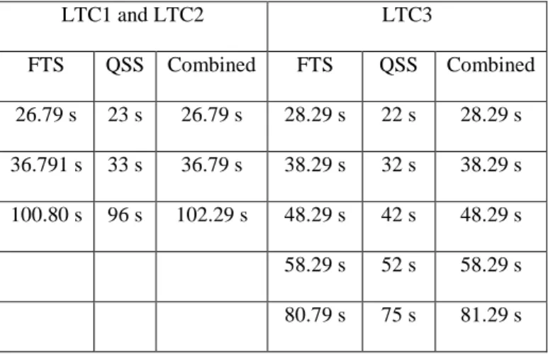
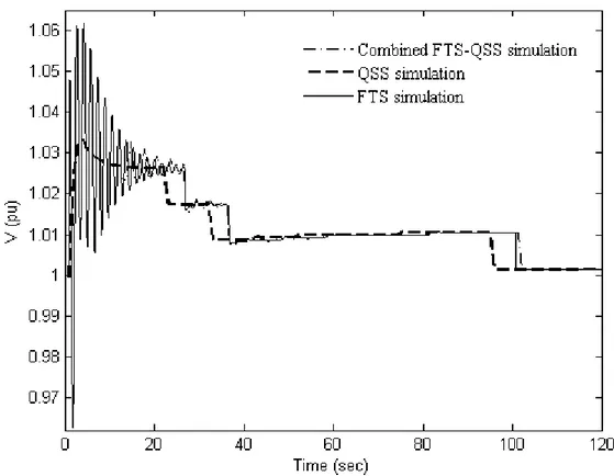
The evolutions of voltage magnitudes at nodes 12 and 20 over a longer time interval are depicted in Figures 11 and 12, respectively, clearly demonstrating that the proposed approach provides similar results to those obtained by the FTS simulation. After the load shedding, large oscillations of voltage magnitudes take place during the short-term period, which are not present in the QSS response, and the voltage magnitude increases due to the reduction in reactive power demand. Since the LTC-controlled voltages are deviated from scheduled values, the tap changers are activated with delays. Times at which the LTCs’ control takes place are reported in Table 1 for each simulation. The control actions occur almost at the same time for the FTS and FTS-QSS simulations. In these cases, controlled voltages re-enter the selected deadbands transiently due to voltage oscillations and delays the LTCs control actions. On the other hand, since the sequence of controls depends on the system dynamics, the LTC’s responses computed by the QSS simulation differ because the short-term dynamics are not considered in the formulation, such that the LTCs move earlier than in the former two simulations.
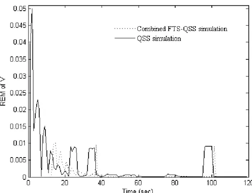
The REM of the dynamic evolutions of voltage magnitudes computed by the FTS-QSS and QSS simulations at buses 12 and 20 are reported in Figures 13 and 14, respectively, with respect to that computed by the FTS simulation. Note that the REMs obtained by the proposed approach are smaller than those obtained by the QSS simulation during the whole period of study, which demonstrate the suitability of the FTS-QSS simulation.
3.2 46- Machine, 190-Bus Mexican power system
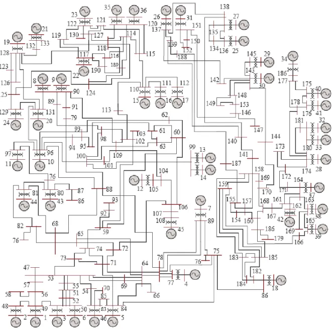
The proposed approach has been applied to a reduced model of the Mexican Interconnected System including the northern, north-eastern, western, central and south-eastern areas, as shown in Figure 15 [18]. This equivalent consists of 190 buses, 46 generators, 90 loads and 265 transmission lines operating at voltage levels ranging from 400 kV to 115 kV. Voltage problems are acute and of prime importance due to the longitudinal structure of the system, such that the load buses 182, 183, and 184 have been equipped with LTCs to maintain voltage magnitude at 1 pu with a half-deadband of ±0.01 pu. The operation of the LTCs start after a first delay of 20 s from the detection of a controlled magnitude voltage outside the deadband, and subsequently each 10 s until the voltage target or the tap ratio limit is achieved. All system data are taken form [19], while the LTCs data are given in Appendix B.
The study scope is to compute the system’s dynamic responses to the following two sequences of disturbances: i) A solid three-phase fault applied at bus 185 at t=1 s and cleared by tripping the line that connects buses 185-189 at t=1.12s; and ii) the tripping at t=6s of the generator connected at bus 18. The analysis is performed over the interval T=[0, 280] s with both FTS and FTS-QSS simulations considering ω0as the rotating frame of reference and assuming that each generator preserves its own rotating speed. The former uses an integration step size of 0.01s, while the proposed FTS-QSS simulation permits the use of a time step of 1s after the switching criterion has been satisfied at t=13.36s considering a switching tolerance of 0.1 and tTOL =0.1s. The fast-state variables monitored to carry out the switching from the FTS to QSS model are those associated with the exciters (Efd), generators (ψ1d, ψ1q, ψ2q), and turbines (PHP,
LP
P ), which satisfy the switching criterion at 3.96s, 8.42s, and 13.36s, respectively.
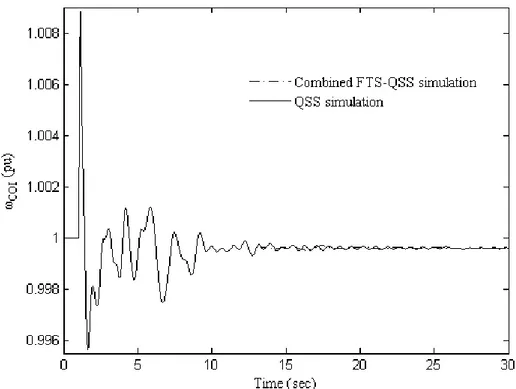
As a result of the first perturbation, the angular speed ωCOI presents large oscillations due to the imbalance of mechanical and electrical powers; but the time at which the fault is cleared allows preserving short-term stability. The second disturbance causes a deviation of ωCOI from the nominal speed ω0, such that the speed governors act to restore the frequency close to its nominal value as shown in Figure 16. For clarity, the ωCOI evolution is plotted for a period of 30s showing that the FTS and combined simulations are very close and tend to the same equilibrium point.
Despite the controlled voltage magnitudes at buses 182, 183 and 184 re-enter the deadbands transiently during the first perturbation, the generator’s tripping causes that these magnitudes drop from their scheduled values due to the reduced voltage support, such that the LTCs act to achieve their control action. Table II reports times of LTC discrete events computed by the FTS and the proposed method. The LTCs installed at buses 182 and 183 detect their controlled voltage magnitudes outside deadbands at 6.01s and 5.36s, respectively, such that taps move after the first delay of 20s
and have discrete changes at 10s intervals. However, the voltage magnitudes cannot be restored, as shown in Figures 17 and 18, due to the LTC lower limit of 0.8 pu being reached at 276.01 s and 265.36 s, respectively. On the other hand, the LTC installed at bus 184 detect the low voltage magnitude at 6.01s and its operation starts after a delay of 20s until its controlled voltage magnitude returns to the deadband at 136.01s. A new degradation of this voltage magnitude occurs due to the actions of LTCs at buses 182 and 183, so that the LTC at bus 184 is activated again and the target voltage is achieved at t=275.37 s with the tap ratio almost at its lower limit. . The evolution of the voltage magnitude at bus 184 is shown in Figure 19 while the changes on the tap ratio of the LTC connected at this node are depicted in Figure 20.
The discrepancy of the results obtained for the voltage magnitude at bus 184 by the FTS and FTS-QSS simulations is shown in Figure 21 in terms of the relative error magnitude: This error appears after the switching from the FTS to QSS simulation takes place but is very small and its evolution presents peaks of small magnitude due to the changes on the tap ratio of each LTC. Based on these simulations, it is numerically confirmed that the FTS-QSS evolution is a very good approximation of the FTS one, such that from a practical viewpoint, the proposed method is suitable for the simulation of long-term dynamics including discrete events.
Lastly, the computing times required by the FTS and FTS-QSS simulations were 200.86s and 17.94s, respectively, being the proposed method 12.31 times faster than the FTS simulation. For these cases, the number of iterations required by the Newton-Raphson method to get to the solution of the linearized set of equations (13) at each time step of both type dynamic simulations is shown in Figure 22. The convergence criterion was 10-6 p.u. These results indicate that the algorithms retain the quadratic convergence of the full Newton-Raphson method and that after a switching takes place, the maximum number of iterations for both simulations is 3. This clearly demonstrates the suitability of the proposed approach to carry out long-term dynamic studies.
4. Conclusions
A new and simple criterion to accurately determine when a QSS model of a power system can be considered as a uniform approximation of the system’s FTS model has been proposed in the paper inspired of Singular Perturbation and two-time scales theories.
On the basis of the suitability of this criterion, an integrated simulation method that combines the reliability of FTS simulation and the efficiency of the QSS simulation has been proposed to speed up the long-term dynamical analysis of power systems considering the presence of discrete events. The method is capable of assessing instability problems
during the short-term period through the FTS simulation. If the fast modes are damped out, a model reduction is automatically carried out to analyze the long-term dynamics by the QSS simulation with larger integration time step sizes.
Simulation results were presented that show the effectiveness of the proposed method and its applicability to efficiently analyze long-term dynamics of a real-life power system. Lastly, an extension of the proposed method would consist in considering different switching times for different components. By so doing, remote parts of the system with little response to the disturbance, could switch earlier under the QSS approximation, which can be seen as an automatic equivalencing.
Appendix
A. One-Machine Infinite-bus system
This Appendix presents data for the simple system. Each transmission line is considered ideal with a series reactance of XL=0.055 pu. Prior to any perturbation, the system is operating at the equilibrium point V∞ = ∠ °1 0 pu and
1 1.0475 3.76
V = ∠ °pu. The machine parameters are the following: Snom=1100MVA, Pnom=935MW, ωs=377rad/s, H=4.2,
D=5, Xs=1.125pu, Xd=1pu, X'd =0.31pu, X''d =0.256pu, T'do =10.2s, T''do=0.0245s, Xq=0.69pu, X'q =0.356pu,
''q
X =0.08pu, T'qo=0.6s, T''qo=0.054s.
B. LTC data
The LTC model data are as follows: rmin=0.8, rmax=1.1, ∆r=0.01, Tf0+Tm=20s, Tf+Tm=10s, d=0.01pu.
References
[1] J.H. Chow (Editor), Time scale modeling of dynamic networks with applications to power systems, Lecture notes in control and information sciences, Berlin:Springer-Verlag, 1982.
[2] M. Stubbe, A. Bihain, J. Deuse, and J.C. Baader, STAG- A new unified software program for the study of the dynamic behaviour of electrical power systems, IEEE Trans. on Power Syst., Vol.4, No.1, (Feb.) (1989), pp. 129-138.
[3] J.Y. Astic, A. Bihain, and M. Jerosolimski, The mixed Adams-BDF variable step size algorithm to simulate transient and long term phenomena in power systems, IEEE Trans. on Power Syst., vol.9, No. 2, (May) (1994), pp. 929-935.
[4] J.J. Sanchez-Gasca, R. D'Aquila, W.W. Price, and J.J. Paserba, Variable time step, implicit integration for extended-term power system dynamic simulation, in: Proc. IEEE Power Industry Computer Application Conf., (1995) pp. 183-189.
[5] R.J. Frowd, J.C. Giri, and R. Podmore, Transient stability and long-term dynamics unified, IEEE Trans. on Power. App. and Syst., Vol. PAS-101, No.10, (Oct.) (1982), pp. 3841-3850.
[6] D. Yang and V. Ajjarapu, A decoupled time-domain simulation method via invariant subspace partition for power system analysis, IEEE Trans. on Power Syst., Vol.21, No.1, (Feb.) (2006), pp. 11-18.
[7] M.-E. Grenier, D. Lefebvre and T. Van Cutsem, Quasi-steady state models for long-term voltage and frequency dynamics simulation, in: Proc. IEEE Power Tech Conf., (2005) pp. 1-8.
[8] L. Loud, P. Rousseaux, D. Lefebvre, and T. Van Cutsem, A time-scale decomposition-based simulation tool for voltage stability analysis, in: Proc. IEEE Power Tech Conf., (2001) pp. 1-6.
[9] T. Van Cutsem, M.–E. Grenier, and D. Lefebvre, Combined detailed and quasi steady-state time simulations for large-disturbance analysis, Int. Journal of Elect. Power and Energy Syst., Vol. 28, No. 9, (Nov.) (2006), pp. 634-642.
[10] X. Xu, R.M. Mathur, J. Jiang, G.J. Rogers, and P. Kundur, Modeling of Generators and Their Controls in Power System Simulations Using Singular Perturbations, IEEE Trans. on Power Syst., Vol. 13, No. 1, (Feb.) (1998), pp. 109-114.
[11] G. Peponides, P. V. Kokotovic, and J. H. Chow, Singular perturbations and time scales in nonlinear models of power systems, IEEE Trans. on Circuits Syst., Vol-CAS-29, No. 11, (Nov.) (1982), pp. 758-767.
[12] E.G. Cate, K. Hemmaplardh, J.W. Manke and D.P. Gelopulos, Time frame notion and time response of the models in transient, mid-term and long term stability programs, IEEE Trans. on Power. App. and Syst., Vol. PAS-103, No.1, (Jan.) (1984), pp. 143-151.
[13] T. Van Cutsem and C. Vournas, Voltage Stability of Electric Power Systems, Massachusetts: Kluwer Academic Publishers, 1998.
[14] F.P. de Mello, J.W. Feltes, T.F. Laskowski and L.J. Oppel, Simulating fast and slow dynamic effects in power systems, IEEE Computer Applications in Power, Vol. 5, No. 3, (July) (1992), pp. 33-38.
[15] P. Kokotovic, H. K. Khalil, and J. O’Reilly, Singular Perturbation Methods in Control: Analysis and Design, London: Academic Press, 1986.
[16] M.A. Pai, Energy function analysis for power system stability, MA: Kluwer, 1989. [17] P. Kundur, Power system stability and control, New York: McGraw-Hill, 1994.
[18] A.R. Messina, and V. Vittal, Assessment of nonlinear interaction between nonlinearly coupled modes using higher order spectra, IEEE Trans. on Power Syst., vol.20, No.1, (Feb.) (2005), pp. 375-383.
Figure captions
:Figure 1. One-machine infinite-bus system.
Figure 2. Terminal voltages and flux linkage at bus 1. Figure 3. New England test system.
Figure 4. Angular speed of the generator connected at bus 34. Figure 5. Field voltage of the generator connected at bus 34.
Figure 6. Individual angular speeds computed by the FTS simulation.
Figure 7. Individual angular speeds computed by the FTS-QSS simulation.
Figure 8. Individual angular speed computed by the QSS simulation.
Figure 9. Angular speed in COI coordinates. Figure 10. Relative error magnitude of the ωCOI
Figure 11. Voltage magnitude at bus 12. Figure 12. Voltage magnitude at bus 20.
Figure 13. Relative error magnitude of voltage magnitude at bus 12. Figure 14. Relative error magnitude of voltage magnitude at bus 20. Figure 15. Schematic diagram of the Mexican power system. Figure 16. Angular speed of the Mexican system in COI coordinates Figure 17. Voltage magnitude at bus 182.
Figure 18. Voltage magnitude at bus 183. Figure 19. Voltage magnitude at bus 184.
Figure 20. Tap ratio evolution of the LTC at bus 184. Figure 21. REM of voltage magnitude at bus 184.
Tables
:Table 1. Activation of LTCS control in New England System
LTC1 and LTC2 LTC3 FTS QSS Combined FTS QSS Combined 26.79 s 23 s 26.79 s 28.29 s 22 s 28.29 s 36.791 s 33 s 36.79 s 38.29 s 32 s 38.29 s 100.80 s 96 s 102.29 s 48.29 s 42 s 48.29 s 58.29 s 52 s 58.29 s 80.79 s 75 s 81.29 s
Table 2. Activation of LTC control in Mexican system (in seconds)
FTS 23.7 33.7 43.7 53.7 63.7 73.7 83.7 93.7 FTS-QSS 25.6 35.5 45.5 55.5 65.5 75.5 85.5 95.7
Figures
:Figure 1. One-machine infinite-bus system.
Figure 3. New England test system.
Figure 4. Angular speed of the generator connected at bus 34.
Figure 5. Field voltage of the generator connected at bus 34.
Figure 7. Individual angular speeds computed by the FTS-QSS simulation.
Figure 9. Angular speed in COI coordinates.
Figure 11. Voltage magnitude at bus 12.
Figure 13. Relative error magnitude of voltage magnitude at bus 12.
Figure 16. Angular speed of the Mexican system in COI coordinates.
Figure 18. Voltage magnitude at bus 183.
Figure 20. Tap ratio evolution of the LTC at bus 184.