arXiv:0908.1553v2 [astro-ph.EP] 25 Nov 2009
Preprint typeset using LA
TEX style emulateapj v. 08/22/09
WASP-17b: AN ULTRA-LOW DENSITY PLANET IN A PROBABLE RETROGRADE ORBIT†
D. R. Anderson1, C. Hellier1, M. Gillon2,3, A. H. M. J. Triaud2, B. Smalley1, L. Hebb4, A. Collier Cameron4, P. F. L. Maxted1, D. Queloz2, R. G. West5, S. J. Bentley1, B. Enoch4, K. Horne4, T. A. Lister6, M. Mayor2,
N. R. Parley4, F. Pepe2, D. Pollacco7, D. S´egransan2, S. Udry2, D. M. Wilson1⋆ Draft version November 25, 2009
ABSTRACT
We report the discovery of the transiting giant planet WASP-17b, the least-dense planet currently known. It is 1.6 Saturn masses but 1.5–2 Jupiter radii, giving a density of 6–14 per cent that of Jupiter. WASP-17b is in a 3.7-day orbit around a sub-solar metallicity, V = 11.6, F6 star. Preliminary detection of the Rossiter–McLaughlin effect suggests that WASP-17b is in a retrograde orbit (λ ≈ −150 deg), indicative of a violent history involving planet–planet or star–planet scattering.
WASP-17b’s bloated radius could be due to tidal heating resulting from recent or ongoing tidal circularisation of an eccentric orbit, such as the highly eccentric orbits that typically result from scattering interactions. It will thus be important to determine more precisely the current orbital eccentricity by further high-precision radial velocity measurements or by timing the secondary eclipse, both to reduce the uncertainty on the planet’s radius and to test tidal-heating models. Owing to its low surface gravity, WASP-17b’s atmosphere has the largest scale height of any known planet, making it a good target for transmission spectroscopy.
Subject headings: planetary systems: individual: WASP-17b – stars: individual: WASP-17
1. INTRODUCTION
The first measurement of the radius and density of an extrasolar planet was made when HD 209458b was seen to transit its parent star (Charbonneau et al. 2000, Henry et al. 2000). The large radius (1.32 RJup) of HD 209458b, confirmed by later observations (e.g., Knut-son et al. 2007), could not be explained by standard models of planet evolution (Guillot & Showman 2002). Since the discovery of HD 209458b, other bloated plan-ets have been found, including TrES-4 (Mandushev et al. 2007), WASP-12b (Hebb et al. 2008), WASP-4b (Wil-son et al. 2008; Gillon et al. 2009a, Winn et al. 2009a, Southworth et al. 2009), WASP-6b (Gillon et al. 2009b), XO-3b (Johns-Krull et al. 2008; Winn et al. 2008) and HAT-P-1b (Bakos et al. 2007; Winn et al. 2007; Johnson et al. 2008). Of those, TrES-4 is the most bloated, with a density 15 per cent that of Jupiter, and a radius larger by a factor 1.78 (Sozzetti et al. 2009).
The mass, composition and evolution history of a planet determines its current radius (e.g., Burrows et al. Electronic address: [email protected]
1Astrophysics Group, Keele University, Staffordshire, ST5 5BG, UK
2Observatoire de Gen`eve, Universit´e de Gen`eve, 51 Chemin des Maillettes, 1290 Sauverny, Switzerland
3Institut d’Astrophysique et de G´eophysique, Universit´e de Li`ege, All´ee du 6 Aoˆut, 17, Bat. B5C, Li`ege 1, Belgium
4School of Physics and Astronomy, University of St. Andrews, North Haugh, Fife, KY16 9SS, UK
5Department of Physics and Astronomy, University of Leicester, Leicester, LE1 7RH, UK
6Las Cumbres Observatory, 6740 Cortona Dr. Suite 102, Santa Barbara, CA 93117, USA
7Astrophysics Research Centre, School of Mathematics & Physics, Queen’s University, University Road, Belfast, BT7 1NN, UK
⋆Present address: Centre for Astrophysics & Planetary Science, University of Kent, Canterbury, Kent, CT2 7NH, UK
†Based in part on data collected with the HARPS spectrograph at ESO La Silla Observatory under programme ID 081.C-0388(A).
2007; Fortney et al. 2007). Recently, numerous theo-retical studies have attempted to discover the reasons why some short-orbit, giant planets are bloated. A small fraction of stellar insolation energy would be sufficient to account for bloating, but no known mechanism is able to transport the insolation energy deep enough within a planet to significantly affect the planet’s evolution (Guil-lot & Showman 2002; Burrows et al. 2007). Enhanced atmospheric opacity would cause internal heat to be lost more slowly, causing a planet’s radius to be larger than otherwise at a given age (Burrows et al. 2007). In-deed, the more highly irradiated planets are thought to have enhanced opacity due to species such as gas-phase TiO/VO, tholins or polyacetylenes (Burrows et al. 2008; Fortney et al. 2008). These upper-atmosphere absorbers result in detectable stratospheres (e.g., Knutson et al. 2009) and prevent incident flux from reaching deep into the atmosphere, causing a large day-night temperature contrast, which leads to faster cooling (Guillot & Show-man 2002). That some planets are not bloated, though they are in similar irradiation environments and have otherwise similar properties to bloated planets, may be due to differences in evolution history or in core mass (Guillot et al. 2006; Burrows et al. 2007).
Currently, the most promising explanation for the large radii of some planets is that they were inflated when the tidal circularisation of eccentric orbits caused energy to be dissipated as heat within the planets (Bodenheimer et al. 2001; Gu et al. 2003; Jackson et al. 2008a; Ibgui & Burrows 2009). Indeed, Jackson et al. (2008b) found that the distribution of the eccentricities of short-orbit (a < 0.2 AU) planets could have evolved, via tidal cir-cularisation, from a distribution identical to that of the farther-out planets.
The angular momenta of a star and its planets derive from that of their parent molecular cloud, so close align-ment is expected between the stellar spin and planetary orbit axes. When a planet obscures a portion of its
par-ent star we observe an apparpar-ent spectroscopic redshift or blueshift; which we see depends on whether the area obscured is approaching or receding relative to the star’s bulk motion. This manifests as an ‘anomalous’ radial velocity (RV) and is known as the Rossiter-McLaughlin (RM) effect (e.g., Queloz et al. 2000a; Gaudi & Winn 2007). The shape of the RM effect is sensitive to the path a planet takes across its parent star, relative to the star’s spin axis. Thus, spectroscopic observation of a transit allows measurement of λ, the sky-projected angle between the stellar spin and planetary orbit axes. Short-orbit, giant planets are thought to have formed just out-side the ice boundary and migrated inwards (e.g., Ida & Lin 2004). Thus, λ is a useful diagnostic for theories of planet migration, some of which predict preservation of initial spin-orbit alignment and some of which would occassionally produce large misalignments. For example, migration via tidal interaction of a giant planet with a gas disc (Lin et al. 1996; Ward 1997) is expected to preserve spin-orbit alignment, whereas migration via a combination of planet-planet scattering and tidal circu-larisation of a resultant eccentric orbit is able to pro-duce a significant misalignment (e.g., Rasio & Ford 1996; Chatterjee et al. 2008; Nagasawa et al. 2008). To date, λ has been determined for 14 systems (Fabrycky & Winn 2009; Gillon 2009; Triaud et al. 2009) and for 3 of those a significant misalignment was found: XO-3b (λ = 37.3±3.7 deg, Winn et al. 2009b; see also: H´ebrard et al. 2008), HD 80606b (λ = 59+28−18deg, Gillon 2009; see also: Moutou et al. 2009; Pont et al. 2009; Winn et al. 2009c) and WASP-14b (λ = −33.1 ± 7.4 deg, Johnson et al. 2009; see also: Joshi et al. 2009).
In this paper, we present the discovery of the transit-ing extrasolar planet WASP-17b, which is the least-dense planet currently known and the first planet found to be in a probable retrograde orbit.
2. OBSERVATIONS
WASP-17 is a V = 11.6, F6 star in Scorpius. It was observed by WASP-South (Pollacco et al. 2006) from 2006 May 04 to 2006 August 18, again from 2007 March 05 to 2007 August 19 and again from 2008 March 02 to 2008 April 19. These observations resulted in 15 509 usable photometric measurements, spanning two years and from two separate fields. A transit search (Collier Cameron et al. 2006) found a strong, 3.7-day periodicity (Figure 1).
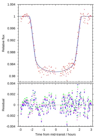
A full transit of WASP-17 was observed in the Ic-band with EulerCAM on the 1.2-m Euler-Swiss telescope on 2008 May 06. The telescope was defocused to give a mean stellar profile width of 4′′. Over a duration of 6 hours, 181 frames were obtained with a range of expo-sure times of 32–98 s — the expoexpo-sure time was tuned to keep the stellar peaks constant. Observations began when WASP-17 was at airmass 1.07; the star then passed through the meridian before reaching airmass 1.8 when observations ended at twilight. The resulting light curve and the residuals about the model fits (§4) are shown in Figure 2 and the photometry is given in Table 1.
Using the CORALIE spectrograph mounted on the Euler-Swiss telescope (Baranne et al. 1996; Queloz et al. 2000b), 5 spectra of WASP-17 were obtained in 2007, 16 more in 2008, and a further 20 in 2009. Three
high--0.08 -0.06 -0.04 -0.02 0 0.02 0.04 0.06 0.08 0.4 0.5 0.6 0.7 0.8 0.9 1 1.1 1.2 1.3 1.4 1.5 1.6 Differential magnitude Orbital phase
Fig. 1.—WASP-South discovery light curve, phase-folded with the ephemeris of Table 4. Points with error > 0.05 mag (3 σmedian) were clipped for display. From the WASP discovery photometry we found a high probability (0.74) of WASP-17 being a main-sequence star and a zero probability of the companion having RP< 1.5 RJup (Collier Cameron et al. 2007). As such, the system did not ful-fill one of our usual selection criteria, P(RP < 1.5 RJup) > 0.2, for follow-up spectroscopy (Collier Cameron et al. 2007). We therefore advise other transit surveys to exercise caution in rejecting candi-dates on the basis of size, so as not to miss interesting systems like WASP-17. -0.004 -0.002 0 0.002 0.004 -3 -2 -1 0 1 2 3 Residual
Time from mid-transit / hours 0.98 0.984 0.988 0.992 0.996 1 1.004 Relative flux
Fig. 2.— Upper panel: Euler Ic-band light curve (red circles) taken on 2008 May 06. Overplotted are the best-fitting model transits (solid lines; §4) from the parameters of Table 4; consult that table for the key to the colour and symbol scheme. Lower panel: Residuals about the model fits. For the green and the magenta models (triangles) the noise is the same (rms = 1140 ppm; red noise = 840 ppm — calculated using the method of Gillon et al. 2006); for the blue model (squares) the noise is slightly higher (rms = 1210 ppm; red noise = 920 ppm, Gillon et al. 2006). The mean theoretical error is 800 ppm.
TABLE 1
Ic-band photometry of WASP-17 HJD–2 450 000 Relative flux σf lux
(days) 4592.677426 0.999803 0.000959 4592.678457 0.998623 0.000956 4592.679703 0.999471 0.000670 . . . . 4592.923564 1.00053 0.00141 4592.926643 1.00034 0.00145
Note. — This table is presented in its en-tirety in the electronic edition of the Astrophysi-cal Journal. A portion is shown here for guidance regarding its form and content.
precision spectra were obtained in 2008 with the HARPS spectrograph (Mayor et al. 2003), based on the 3.6-m ESO telescope. RV measurements were computed by weighted cross-correlation (Baranne et al. 1996; Pepe et al. 2005) with a numerical G2-spectral template. RV variations were detected with the same period found from the WASP photometry and with semi-amplitude of ∼50 m s−1, consistent with a planetary-mass companion. The RV measurements are listed in Table 2 and are plot-ted in Figure 3.
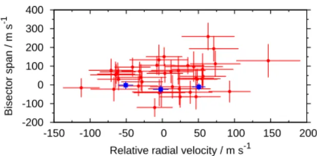
To test the hypothesis that the RV variations are due to spectral line distortions caused by a blended eclipsing binary, a line-bisector analysis (Queloz et al. 2001) of the CORALIE and HARPS cross-correlation functions was performed. The lack of correlation between bisec-tor span and radial velocity (Figure 4), especially for the high precision HARPS measurements, supports the iden-tification of the transiting body as a planet.
3. STELLAR PARAMETERS
The combined CORALIE and HARPS spectra from 2007–2008, co-added into 0.01˚A steps, give a S/N of ∼100:1. The stellar parameters and elemental abun-dances of WASP-17 were determined using spectrum syn-thesis and equivalent-width measurements (Gillon et al. 2009b; West et al. 2009) and are given in Table 3. In the spectra, the Li i 6708˚A line is not detected (EW < 2m˚A), giving an upper-limit on the Lithium abun-dance of log n(Li/H) + 12 < 1.3. However, the effective temperature of this star implies it is in the lithium-gap (B¨ohm-Vitense 2004) and so the lithium abundance does not provide an age constraint. In determining the pro-jected stellar rotation velocity (v sin i) from the HARPS spectra, a value for macroturbulence (vmac) of 6 km s−1 was adopted (Gray 2008) and an instrumental FWHM of 0.06˚A, determined from the telluric lines around 6300˚A, was used. A best fitting value of v sin i = 9.0 ± 1.5 km s−1 was obtained. However, if vmacis lower than the assumed 6 km s−1 then v sin i would be slightly higher, with a value of 11 km s−1 obtained if v
mac is assumed to be zero.
We attempted to measure the rotation period of WASP-17 by searching for sinusoidal, rotational mod-ulation of the WASP light curve (Hebb et al. 2009), as may be induced by a non-axisymmetric distribution of starspots. Considering periods of 1.05–30 days, the best-fitting period is 24.7 days. However, the amplitudes of the phase-folded light curves from each camera from
-100 -50 0 50 100 150 0.4 0.5 0.6 0.7 0.8 0.9 1 1.1 1.2 1.3 1.4 1.5 1.6 Residual / m s -1 Orbital phase -150 -100 -50 0 50 100 150 200 250
Relative radial velocity / m s
-1
Fig. 3.— Upper panel: Relative radial velocity measurements of WASP-17 as measured by CORALIE (red circles). The three, colour-coded solid lines are the model orbital solutions (§4) based on the parameters of Table 4 and incorporate the RM effect. As the zero-point offset between HARPS and CORALIE is a free pa-rameter in the models, the HARPS measurements are shown once per model, with corresponding symbols and colours (Table 4). The centre-of-mass velocities of Table 4 have been subtracted. Lower panel: Residuals about the model solutions; consult Table 4 for the key to the symbol and colour scheme.
-200 -100 0 100 200 300 400 -150 -100 -50 0 50 100 150 200 Bisector span / m s -1
Relative radial velocity / m s-1
Fig. 4.— Bisector span versus relative radial velocity for the CORALIE (red circles) and HARPS (blue squares) spectra. Av-erages of the centre-of-mass velocities and zero-point offsets of Ta-ble 4 were subtracted. Bisector uncertainties equal to twice the radial velocity uncertainties have been adopted. The Pearson cor-relation coefficient is 0.19.
TABLE 2
Radial velocity measurements of WASP-17
BJD–2 450 000 RV σRV BSa (km s−1) (km s−1) (km s−1) CORALIE: 4329.6037 –49.4570 0.0428 0.0829 4360.4863 –49.3661 0.0444 0.1290 4362.4980 –49.5175 0.0407 0.1335 4364.4880 –49.4891 0.0432 –0.0213 4367.4883 –49.4415 0.0343 0.1931 4558.8839 –49.4988 0.0311 –0.0101 4559.7708 –49.5798 0.0325 –0.0229 4560.7314 –49.5734 0.0295 0.0303 4588.7799 –49.4881 0.0289 –0.0638 4591.7778 –49.4661 0.0340 –0.0631 4622.6917 –49.3976 0.0351 0.1071 4624.6367 –49.4494 0.0367 0.2581 4651.6195 –49.4564 0.0319 0.0459 4659.5246 –49.4693 0.0405 0.0972 4664.6425 –49.5424 0.0353 0.0401 4665.6593 –49.4905 0.0377 0.0770 4682.5824 –49.5007 0.0309 0.0707 4684.6264 –49.5169 0.0357 –0.0418 4685.5145 –49.4741 0.0307 –0.0393 4690.6182 –49.5776 0.0350 0.0541 4691.6077 –49.5140 0.0406 –0.0380 4939.8457 –49.4394 0.0349 0.1127 4940.7346 –49.5838 0.0309 0.0777 4941.8520 –49.5408 0.0290 0.0163 4942.6959 –49.4775 0.0227 0.1030 4942.8747 –49.4196 0.0291 –0.0355 4943.6655 –49.5103 0.0253 0.1504 4943.8872 –49.5885 0.0268 0.0732 4944.6858 –49.5540 0.0250 0.0951 4944.8689 –49.5746 0.0249 0.0694 4945.6969 –49.5442 0.0252 0.0727 4945.8277 –49.5767 0.0263 0.0579 4946.7289 –49.4662 0.0251 0.0351 4946.9069 –49.4578 0.0256 0.0326 4947.6558 –49.5028 0.0261 –0.1128 4947.8694 –49.5092 0.0251 0.0614 4948.6415 –49.5203 0.0251 0.1043 4948.8836 –49.6250 0.0254 –0.0153 4949.8646 –49.4643 0.0279 0.0307 4951.6661 –49.5233 0.0250 –0.1208 4951.8719 –49.5458 0.0271 –0.0061 HARPS: 4564.8195 –49.4884 0.0108 –0.0239 4565.8731 –49.4356 0.0092 –0.0103 4567.8516 –49.5368 0.0105 –0.0015 aBS: bisector span
each season are small (2–8 mmag). Assuming spin-orbit alignment, with v sin i = 9.0 km s−1, and using the val-ues of stellar radius given in Table 4 (see §4), a stellar rotation period of 8.5–11 days is expected.
We estimated the distance of WASP-17 (400 ± 60 pc) using the distance modulus, the TYCHO apparent visual magnitude (V = 11.6) and the absolute visual magnitude of an F6V star (V = 3.6; Gray 2008); we assumed E(B − V ) = 0.
4. SYSTEM PARAMETERS
The WASP-South and EulerCAM photometry were combined with the CORALIE and HARPS RV mea-surements in a simultaneous Markov-chain Monte-Carlo (MCMC) analysis (Collier Cameron et al. 2007; Pollacco
TABLE 3
Stellar parameters of WASP-17
Parameter Value Teff (K) 6550 ± 100 log g∗(cgs) 4.2 ± 0.2 ξt (km s−1) 1.6 ± 0.2 v sin i (km s−1) 9.0 ± 1.5 Spectral Type F6 [Na/H] −0.15 ± 0.06 [Mg/H] −0.21 ± 0.07 [Al/H] −0.38 ± 0.05 [Si/H] −0.18 ± 0.09 [Ca/H] −0.08 ± 0.14 [Sc/H] −0.20 ± 0.14 [Ti/H] −0.20 ± 0.12 [V/H] −0.38 ± 0.13 [Cr/H] −0.23 ± 0.14 [Fe/H] −0.25 ± 0.09 [Ni/H] −0.32 ± 0.11 log N (Li) < 1.3 V (mag) 11.6 Distance (pc) 400 ± 60 R.A. (J2000) = 15h59m50.94s Dec. (J2000) = –28◦03′ 42.3′′ 1SWASP J155950.94−280342.3 USNO-B1.0 0619-0419495 2MASS 15595095−2803422
et al. 2008). The proposal parameters we use are: Tc, P , ∆F , T14, b, K1, M∗, e cos ω, e sin ω, v sin i cos λ and v sin i sin λ. Here Tc is the epoch of mid-transit, P is the orbital period, ∆F is the fractional flux-deficit that would be observed during transit in the absence of limb-darkening, T14is the total transit duration (from first to fourth contact), b is the impact parameter of the planet’s path across the stellar disc, K1is the stellar reflex veloc-ity semi-amplitude, M∗is the stellar mass, e is the orbital eccentricity and ω is the argument of periastron.
At each step in the MCMC procedure, each proposal parameter is perturbed from its previous value by a small, random amount. From the proposal parameters, model light and RV curves are generated and χ2 is cal-culated from their comparison with the data. A step is accepted if χ2is lower than for the previous step; a step with higher χ2may also be accepted, the probability for which is lower for larger ∆χ2. In this way, the param-eter space around the optimum solution is thoroughly explored. Provided the probability of accepting a step of higher χ2 is chosen correctly, then the distribution of points for an MCMC chain gives the standard errors on the parameters (e.g., Ford 2006).
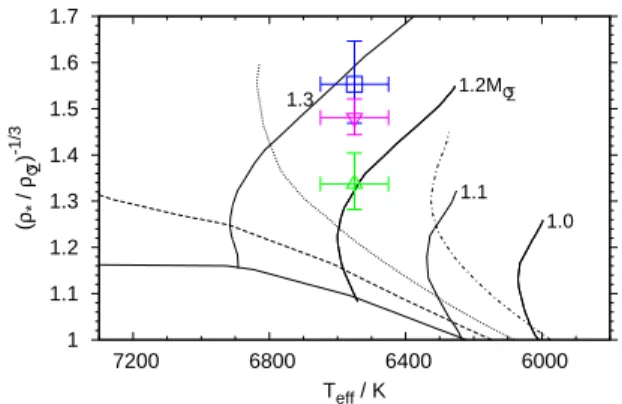
We place a prior on M∗ that, via a Bayesian penalty, causes its values in accepted MCMC steps to approxi-mate a Gaussian distribution with mean M0 and stan-dard deviation σM = 0.1 M0, where M0 is the initial estimate of M∗. To determine M0 and to estimate the star’s age, an evolutionary analysis (Hebb et al. 2008) was performed. In that, an initial MCMC run was used to determine the stellar density, which depends on the shape of the transit light curve and the eccentric-ity of the orbit. The stellar evolution tracks of Girardi et al. (2000) were then interpolated using this stellar density and using the stellar temperature and
metal-licity from the spectral analysis (Figure 5). This sug-gests that WASP-17 has evolved off the zero-age main sequence, with a mass of 1.20+0.10−0.11M⊙ and an age of 3.0+0.9−2.6Gyr. This stellar mass was used as the initial es-timate, M0, in the MCMC solution (Case 1) presented in the second column of Table 4. The best-fitting ec-centricity is non-zero at the 2-σ level (e = 0.129+0.106−0.068; ω = 290+106−16 deg). The best-fitting planet radius is large but uncertain (RP = 1.74+0.26−0.23RJup). This uncertainty results from e and ω being poorly constrained by the RV data, causing the velocity of the planet during transit, and therefore the distance travelled (i.e. the stellar ra-dius), to be uncertain. The planet radius is related to the stellar radius by the measured depth of transit, so it too is uncertain. 1 1.1 1.2 1.3 1.4 1.5 1.6 1.7 6000 6400 6800 7200 ( ρ* / ρO• ) -1/3 Teff / K 1.3 1.2MO• 1.1 1.0
Fig. 5.—Modified H-R diagram: inverse cube-root of stellar den-sity versus stellar effective temperature. The former quantity is purely observational, measured directly from the light curve in ini-tial MCMC runs. The latter quantity is derived from the spectral analysis. The best-fitting values of the three models for WASP-17 are depicted using the key of Table 4. Evolutionary mass tracks (solid, labelled lines) and isochrones (100 Myr, solid; 1 Gyr, dashed; 2 Gyr, dotted; 4 Gyr, dot-dashed) from Girardi et al. (2000) for [Fe/H] = −0.25 are plotted for comparison.
The stellar age from the first MCMC solution and v sin i from the spectral analysis are consistent with WASP-17 being young. As such, a second MCMC anal-ysis was performed, with a main sequence (MS) prior on the star and with eccentricity a free parameter. With the MS prior, a Bayesian penalty ensures that, in ac-cepted steps, the values of stellar radius are consistent with those of stellar mass for a main-sequence star: the probability distribution of R∗ has a mean of R0= M00.8 (Tingley & Sackett 2005), where R0is the initial estimate of R∗, and a standard deviation of σR= 0.8(R0/M0)σM. An initial MCMC analysis was used to determine stel-lar density, which was used as an input to an evolution-ary analysis (Figure 5). That suggests a stellar mass of 1.19+0.07−0.08M⊙and a stellar age of 1.2+2.8−1.2Gyr. This stellar mass was used as the start value in the MCMC solution (Case 2) presented in the third column of Table 4. The MS prior results in a smaller stellar radius and, there-fore, a smaller planetary radius (RP= 1.51 ± 0.10 RJup). The MS prior on stellar radius, together with the prior on stellar mass, effectively places a prior on stellar den-sity, ρ∗, forcing stellar density toward the higher values
typical of a MS star. Therefore, as ρ∗∝
(1 − e2)3/2
(1 + e sin ω)3 (1)
a more eccentric orbit (e = 0.237+0.068−0.069; ω = 278.0+8.2−5.6deg) results. The uncertainties on each of the parameters affected by the MS prior are artificially small due to the MS prior not taking full account of uncer-tainties involved (e.g., in the theoretical mass-radius re-lationship).
As the detection of a non-zero eccentricity in the first MCMC solution is of low significance, a third solution was generated, with an imposed circular orbit and no MS prior. Again, an initial MCMC analysis was performed to determine stellar density, which was used as an input to an evolutionary analysis (Figure 5). From that, a stellar mass of 1.25 ± 0.08 M⊙ and a stellar age of 3.1+1.1−0.8Gyr was found. This stellar mass was used as the start value in the MCMC solution (Case 3) presented in the fourth column of Table 4. The circular orbit causes the velocity of the planet during transit to be higher than in the two eccentric solutions. This results in a larger stellar radius and, as the depth of transit is fixed by measurement, in a larger planet radius (RP= 1.97 ± 0.10 RJup).
For each model, the best-fitting transit light curve is shown in Figure 2 and the best-fitting RV curve is shown in Figure 3. To help decide between the three cases pre-sented, a more precise determination of stellar age, stel-lar radius or orbtial eccentricity would be useful. It is currently difficult to reliably determine the age of stars older than 1–2 Gyr (e.g., Sozzetti et al. 2009 and refer-ences therein). Stellar radius could be calculated from a precise parallax determination. WASP-17’s parallax is predicted to be 2.5 mas, which will be measurable to good precision by the forthcoming Gaia mission (Jordi et al. 2006), which is expected to achieve an accuracy of 7 µas at V = 10. Eccentricity can be better determined using a combination of two methods: (i) Take a number of high-precision RV measurements (which best constrain e sin ω), focusing on those phases at which the differences between the models are greatest (Figure 3). (ii) Observe the secondary eclipse; the time of mid-eclipse constrains e cos ω and the eclipse duration more weakly constrains e sin ω (Charbonneau et al. 2005).
We adopt Case 1 as our preferred solution; we note that if WASP-17 proves to be young then Case 2 will be indicated, and Case 3 will be indicated if the planet’s orbit is found to be (near-)circular.
4.1. A retrograde orbit?
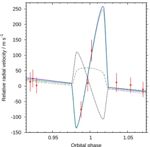
The RM effect was incorporated in the MCMC anal-yses with free parameters v sin i cos λ and v sin i sin λ (Figure 6; Table 4). The three RV measurements during transit suggest a large spin-orbit misalignment (λ ≈ −150 deg), indicating that the planet is orbiting in a sense counter to that of stellar rotation. The RV RMS about the fitted model is 31.6 m s−1. Comparing a borderline prograde-retrograde orbit (λ = −90 deg, v sin i = 9.0 km s−1, b = 0.355), the first in-transit point is discrepant by 5.0 σ and the RV RMS is 40.2 m s−1 (Figure 6). Comparing a prograde orbit (λ = 0 deg, v sin i = 9.0 km s−1, b = 0.355), the first and third
in-transit points are discrepant by 6.0 σ and 3.8 σ respec-tively, and the RV RMS is 45.7 m s−1(Figure 6).
The fitted amplitude of the RM effect suggests v sin i ≈ 20 km s−1, which is higher than determined in the spec-tral analysis (Table 3). This could be because the am-plitude of the RM effect is currently liable to be over-estimated (Winn et al. 2005; Triaud et al. 2009), due to the manner in which the RVs are extracted from the spectra. At present, the effective velocity of the spectro-scopic cross-correlation function (CCF) is measured by fitting a gaussian. However, at values of v sin i signifi-cantly greater than the intrinsic width of the CCF for a slowly-rotating star, the travelling bump in the profile that is the spectral signature of the planet’s silhouette becomes partially resolved (Gaudi & Winn 2007). The CCF profile will become slightly asymmetric when the planet is near the limb, and this may bias the velocity measured by gaussian-fitting to a greater value than the RV of the centroid of the unobscured parts of the star.
-150 -100 -50 0 50 100 150 200 250 0.95 1 1.05
Relative radial velocity / m s
-1
Orbital phase
Fig. 6.—Zoom-in on the spectroscopic transit region of Figure 3, showing the fitted RM effect more clearly. The red circles are CORALIE measurements and the coloured lines are the best-fitting models (Table 4). We show for comparison the RM effects that would result from perpendicular (λ = −90 deg; black, dot-dashed line) and aligned (λ = 0 deg; black, dashed line) spin-orbit axes; in both cases v sin i = 9.0 km s−1and b = 0.355 were fixed.
4.2. Transit times
We measured the times of WASP-17b’s transits to search for transit timing variations, as may be induced by a third body (e.g., Holman & Murray 2005; Agol et al. 2005). The model light curves were stepped in time over the phometric data around the predicted times of transit, and χ2 was calculated at each step. The times of mid-transit were found by measuring the χ2minima and the uncertainties were determined via bootstrapping. The calculated times of mid-transit, Tc, and the differences, O − C, between those times and the predicted times, as-suming a fixed epoch and period (Table 4), are given in Table 5. No significant departure from a fixed ephemeris is seen.
5. DISCUSSION
WASP-17b is the least dense planet known, with a den-sity of 0.06–0.14 ρJ. TrES-4, the previous least dense planet, has a density of 0.15 ρJ (Sozzetti et al. 2009), and HD 209458b, the most studied transiting planet, has a density of 0.27 ρJ (Torres et al. 2008). WASP-17b’s radius of 1.5-2 RJup is larger than predicted by standard planet evolution models. For example those of Fortney et al. (2007) imply a radius of at most 1.3 RJup (the value for a 1-Gyr-old, coreless planet of 0.41 MJup, receiving more stellar flux, at a distance of 0.02 AU, where each of these values errs on the side of inflating the radius).
Burrows et al. (2007) showed that an enhanced atmo-spheric opacity can delay radius shrinkage, leading to a larger-than-otherwise planet radius at a given age. En-hanced opacities may result from super-solar metallicity, the presence of clouds/hazes, or the effects of photol-ysis or non-equilibrium chemisty. One might expect a low planetary atmospheric opacity due to the sub-solar metallicity of the WASP-17 star: [Fe/H] = –0.25. How-ever, as WASP-17b is highly irradiated, its atmospheric opacity is expected to be high due, for example, to the presence of TiO and VO gases (Burrows et al. 2008; Fortney 2008). Ibgui & Burrows (2009) found that an atmospheric opacity of 3 × solar is sufficient to account for the radius of HD 209458b. The very large radius of WASP-17b and its moderate age suggest that enhanced opacity alone, even of 10×solar, is insufficient to account for the planet’s bloatedness.
It has been proposed (Bodenheimer et al. 2001; Gu et al. 2003; Jackson et al. 2008a) that tidal dissipa-tion associated with the circularisadissipa-tion of an eccentric orbit is able to substantially inflate the radius of a short-orbit, giant planet. If a planet is in a close (a < 0.2 AU), highly eccentric (e > 0.2) orbit then planetary tidal dissi-pation will be significant and will shorten and circularise the orbit. Orbital energy is deposited within the planet interior, leading to an inflated planet radius. This pro-cess is accelerated by higher atmospheric opacities: as the planet better retains heat, shrinking of the radius is retarded, and a larger radius causes greater tidal dis-sipation. Higher eccentricities result in stronger tides, and thus in greater tidal dissipation. The rate at which energy is tidally dissipated within a body is inversely pro-portional to its tidal quality factor, Q′, which is the ratio of the energy in the tide to the tidal energy dissipated within the body per orbit (e.g., Ogilvie & Lin 2007).
Ibgui & Burrows (2009) created a tidal dissipation model and applied it to HD 209458b, which is bloated to a lesser degree than WASP-17b. A custom fit is re-quired to find possible evolution histories for the WASP-17 system, but the similarity of HD 209458 (compare Tables 3 and 4 from this paper with Table 1 in Ibgui & Burrows (2009) and references therein) permits com-parison. Ibgui & Burrows’ (2009) HD 209458b model suggests that tidal heating could produce even WASP-17b’s maximum likely radius (RP≈2 RJup) if, for exam-ple, it evolved from a highly eccentric (e ≈ 0.79), close (a ≈ 0.085 AU) orbit, with moderate tidal dissipation (Q′
P ≈106.55; Q′∗ ≈107.0) and solar atmospheric opac-ity. The final semimajor axis of this particular model was shorter than that of WASP-17b, but within 10 per cent. Such an eccentric, short orbit seems reasonable as
TABLE 4
System parameters of WASP-17
Parameter Case 1 (adopted) Case 2 Case 3
Extra constraints . . . MS prior e = 0
Graph colour blue green magenta
Graph symbol squares upwards triangles downwards triangles
Graph line solid dashed dotted
Stellar age (Gyr) 3.0+0.9−2.6 1.2
+2.8 −1.2 3.1 +1.1 −0.8 P (d) 3.7354417+0.0000072−0.0000073 3.7354417+0.0000073−0.0000074 3.7354414+0.0000074−0.0000074 Tc(HJD) 2454559.18102+0.00028−0.00028 2454559.18100 +0.00027 −0.00028 2454559.18096 +0.00028 −0.00028 T14(d) 0.1822+0.0019−0.0023 0.1825 +0.0017 −0.0017 0.1824 +0.0016 −0.0016 T12= T34(d) 0.0235+0.0019−0.0030 0.0236+0.0017−0.0018 0.0239+0.0017−0.0017 ∆F = R2 P/R 2 ∗ 0.01672 +0.00029 −0.00035 0.01674 +0.00027 −0.00027 0.01678 +0.00026 −0.00027 b ≡ a cos i/R∗ 0.352+0.075−0.316 0.355 +0.068 −0.111 0.370 +0.064 −0.096 K1 (km s−1) 0.0569+0.0055−0.0053 0.0592 +0.0058 −0.0057 0.0564 +0.0051 −0.0051 γ (km s−1) -49.5128+0.0016 −0.0016 -49.5128 +0.0014 −0.0014 -49.5125 +0.0014 −0.0015 γHARPS−γCOR.(km s−1) 0.0267+0.0034−0.0035 0.0297 +0.0023 −0.0023 0.0233 +0.0015 −0.0015 a (AU) 0.0501+0.0017−0.0018 0.0494+0.0017−0.0018 0.0507+0.0017−0.0018 i (deg) 87.8+2.0 −1.0 88.16 +0.58 −0.45 86.95 +0.87 −0.63 e cos ω 0.036+0.034−0.031 0.034+0.025−0.024 . . . e sin ω −0.10+0.13−0.13 −0.233 +0.071 −0.070 . . . e 0.129+0.106−0.068 0.237 +0.068 −0.069 0. (fixed) ω (deg) 290+106−16 278.0+8.2−5.6 . . . φmid-eclipse 0.523+0.021−0.020 0.522 +0.016 −0.015 0.5 (fixed) T58(d)a 0.152+0.040−0.034 0.117 +0.017 −0.015 0.1824 +0.0016 −0.0016 (fixed) T56= T78(d)b 0.0186+0.0063−0.0046 0.0140+0.0022−0.0019 0.0239+0.0017−0.0017 (fixed) λ (deg) −147+49−11 −148.7 +13.7 −9.3 −149.3 +11.5 −8.9 v sin i (km s−1) 20.0+69.2 −5.2 19.1 +5.7 −4.8 19.1 +5.3 −4.7 M∗( M⊙) 1.20+0.12−0.12 1.16 +0.12 −0.12 1.25 +0.13 −0.13 R∗( R⊙) 1.38+0.20−0.18 1.200 +0.081 −0.080 1.566 +0.073 −0.073 log g∗(cgs) 4.23+0.12−0.12 4.341+0.068−0.068 4.143+0.032−0.031 ρ∗(ρ⊙) 0.45+0.23−0.15 0.67 +0.16 −0.13 0.323 +0.035 −0.028 MP(MJup) 0.490+0.059−0.056 0.496 +0.064 −0.060 0.498 +0.059 −0.056 RP (RJup) 1.74+0.26−0.23 1.51 +0.10 −0.10 1.97 +0.10 −0.10 log gP (cgs) 2.56+0.14−0.13 2.696 +0.086 −0.083 2.466 +0.051 −0.052 ρP (ρJ) 0.092+0.054−0.032 0.144 +0.042 −0.031 0.0648 +0.0106 −0.0090 TP,A=0(K) 1662+113−110 1557 +55 −55 1756 +26 −30
Three solutions are presented (Cases 1, 2 and 3), each with different constraints as described in the text (§4).
aT
TABLE 5 Transit times Ntr Tc σTc O − C (HJD) (min) (min) −179 2453890.54850 6.2 16.6 −175 2453905.48193 5.5 4.7 −171 2453920.42243 3.6 2.8 −159 2453965.23733 5.0 −12.2 −96 2454200.57081 4.4 −11.2 −92 2454215.52194 2.7 2.3 −77 2454271.55701 4.1 7.2 −73 2454286.49409 8.3 0.5 −69 2454301.45133 8.2 22.8 −61 2454331.32310 9.3 5.8 −1 2454555.43662 6.4 −12.9 2 2454566.65046 8.3 −2.0 9 2454592.80049 0.55 0.79
planets in highly eccentric, quite short orbits are known: HD 17156b (e = 0.676, a = 0.162 AU; Winn et al. 2009d), HD 37605b (e = 0.74, a = 0.26 AU; Cochran et al. 2004), HD 80606b (e = 0.934, a = 0.45 AU; Moutou et al. 2009). As for the strength of tidal dissipation, Jackson et al. (2008b) found similar best-fitting values (Q′
P = 106.5; Q′∗ = 105.5) when matching the current eccentricities of short-orbit (a < 0.2 AU) planets with the eccentricities of farther out planets, from which they presumably evolved.
The limited radial-velocity measurements during tran-sit give a strong indication that WASP-17b is in a retro-grade orbit. As the angular momenta of a star, its proto-planetary disc, and hence its planets, all derive from that of the parent molecular cloud, WASP-17b presumably originated in a prograde orbit. As a gas giant, WASP-17b is expected to have formed just outside the ice boundary (∼3 AU) and migrated inwards to its current separation of 0.05 AU (e.g., Ida & Lin 2004). Migration of a giant planet via tidal interaction with a gas disc is expected to preserve spin-orbit alignment (Lin et al. 1996; Ward 1997) and is thus unable to produce a retrograde orbit. Alternatively, migration via a combination of star-planet scattering (Takeda et al. 2008) or planet-planet scat-tering (e.g., Rasio & Ford 1996; Chatterjee et al. 2008; Nagasawa et al. 2008) and tidal circularisation of the resultant eccentric orbit is able to produce significant misalignment.
In addition to inclined orbits, scattering is able to pro-duce highly eccentric orbits (e.g., Ford & Rasio 2008), which have been found to be common and are neces-sary if tidal circularisation is to inflate planetary radii (e.g., Jackson et al. 2008b), whereas planet-disc interac-tions seem unable to pump eccentricities to large values (e > 0.3; D’Angelo et al. 2006). Nagasawa et al. (2008) carried out orbital integrations of three-planet systems: three Jupiter-mass planets were initially placed beyond the ice boundary (5 AU, 7.25 AU, 9.5 AU) in circular orbits, with small inclinations (0.5◦, 1◦, 1.5◦), around a solar-mass star. They found that a combination of planet-planet scattering, the Kozai mechanism (the os-cillation of the eccenticity and inclination of a planet’s or-bit via the secular perturbation from outer bodies; Kozai
1962) and tidal circularisation produces short-orbit, gi-ant planets in ∼30% of cases. The Kozai mechanism is most effective when the scattered, inner planet has an inclined orbit. A broad spread was seen in the in-clination distribution of the short-orbit planets formed, including planets in retrograde orbits. Therefore, we sug-gest that WASP-17b supports the hypothesis that some short-orbit, giant planets are produced by a combina-tion of scattering, the Kozai mechanism and tidal circu-larisation. The observation of the RM effect for more short-orbit planets is required to measure the size of the contribution.
For planet-planet or star-planet scattering to have in-fluenced WASP-17b’s orbit in the past, one or more stel-lar or planetary companions must have been present in the system. Sensitive imaging could probe for a stel-lar companion and further radial velocity measurements are necessary to search for stellar or planetary compan-ions. It will be worthwhile looking for long-term trends in the RVs to detect farther-out planets that might have been involved in past scattering. A straight-line fit to the residuals of the RV data about the model fits indicates no significant drift over a span of 622 days (e.g., for Case 1 the drift is −17 ± 11 m s−1). In their three-planet in-tegrations, Nagasawa et al. (2008) found that in 75% of cases one planet is ejected, a planet collides with the host star in 22% of cases, and two planets are ejected in 5% of cases. They also found that, since a small difference in orbital energy causes a large difference in semimajor axis in the outer region, the final semimajor axes of outer planets are widely distributed (peak at ∼15 AU, with a large spread). Therefore, it is possible that WASP-17 is now the only giant planet in the system or that the outer planets are in long orbits, which are difficult to detect with the RV technique.
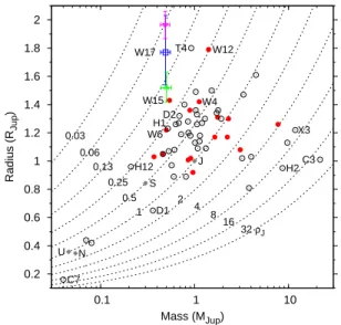
The discovery of WASP-17b extends the mass-radius distribution of the 62 known transiting exoplanets (Fig-ure 7). WASP-17b has the largest atmospheric scale height (1100–2100 km) of any known planet by up to a factor 2, due to its very low surface gravity and mod-erately high equilibrium temperature. The ratio of pro-jected areas of planetary atmosphere to stellar disc of WASP-17b is 1.9–2.7 times that of HD 209458b and 2.4– 3.4 times that of HD 189733b, for both of which success-ful attempts at measuring atmospheric signatures have been made (e.g., Charbonneau et al. 2002, Desert et al. 2009). Thus, although WASP-17 is fainter and has a larger stellar radius, the system is a good prospect for transmission spectroscopy.
6. ACKNOWLEDGEMENTS
We acknowledge a thorough and constructive report from the anonymous referee. The WASP consortium comprises the Universities of Keele, Leicester, St. An-drews, the Queen’s University Belfast, the Open Univer-sity and the Isaac Newton Group. WASP-South is hosted by the South African Astronomical Observatory and we are grateful for their support and assistance. Funding for WASP comes from consortium universities and from the UK’s Science and Technology Facilities Council.
REFERENCES Agol, E., Steffen, J., Sari, R., & Clarkson, W., 2005, MNRAS,
0.2 0.4 0.6 0.8 1 1.2 1.4 1.6 1.8 2 0.1 1 10 Radius (R Jup ) Mass (MJup) 0.03 0.06 0.13 0.25 0.5 1 2 4 8 16 32 ρJ J S N U T4 W12 W6 W4 X3 H1 D1 D2 W15 W17 C7 C3 H2 H12
Fig. 7.— Mass-radius distribution of the 62 known transiting extrasolar planets. The best-fitting values for the three WASP-17b models are depicted according to the key given in Table 4. Other WASP planets are filled, red circles; non-WASP planets are open, black circles; Jupiter, Saturn, Neptune and Uranus are filled, grey diamonds, labelled with the planets’ initials. For clarity, er-ror bars are displayed only for WASP-17b. Some planets discov-ered by CoRoT, HAT, TrES, WASP and XO are labelled with the project initial and the system number (e.g., WASP-17b = W17). HD 149026b is labelled D1 and HD 209458b is labelled D2. The labelled, dashed lines depict a range of density contours in Jovian units. Data are taken from this work and http://exoplanet.eu.
Baranne, A. et al., 1996, A&AS, 119, 373
Bodenheimer, P., Lin, D. N. C., & Mardling, R. A., 2001, ApJ, 548 466
B¨ohm-Vitense, E., 2004, AJ, 128, 2435
Burrows, A., Hubeny, I., Budaj, J., & Hubbard, W. B., 2007, ApJ, 661, 502
Burrows, A., Budaj, J., & Hubeny, I., 2008, ApJ, 678, 1436 Charbonneau, D., Brown, T. M., Latham, D. W., & Mayor, M.,
2000, ApJ, 529, L45
Charbonneau, D., Brown, T. M., Noyes, R. W., & Gilliland, R. L. 2002, ApJ, 568, 377
Charbonneau D. et al., 2005, ApJ, 626, 523
Chatterjee, S., Ford, E. B., Matsumura, S., & Rasio, F. A, 2008, ApJ, 686, 580
Cochran, W. D. et al., 2004, ApJ, 611, L133 Collier Cameron, A. et al., 2006, MNRAS, 373, 799 Collier Cameron, A. et al., 2007, MNRAS, 380, 1230
D’Angelo, G., Lubow, S. H., & Bate, M. R., 2006, ApJ, 652, 1698 Desert, J.-M., Lecavelier des Etangs, A., Hebrard, G., Sing,
D. K., Ehrenreich, D., Ferlet, R., & Vidal-Madjar, A., 2009, ApJ, 699, 478
Fabrycky, D. C., & Winn, J. N., 2009, ApJ, 696, 1230 Ford, E. B., 2006, ApJ, 642, 505
Ford, E. B., & Rasio, F. A., 2008, ApJ, 686, 621
Fortney, J. J., Marley, M. S., & Barnes, J. W., 2007, ApJ, 659, 1661
Fortney, J. J., Lodders, K., Marley, M. S., & Freedman, R. S., 2008, ApJ, 678, 1419
Gaudi, B. S., & Winn, J .N., 2007, ApJ, 655, 550
Gillon, M., Pont, F., Moutou, C., Bouchy, F., Courbin, F., Sohy, S., & Magain, P. 2006, A&A, 459, 249
Gillon, M., 2009, arXiv:0906.4904 Gillon, M. et al., 2009a, A&A, 496, 259 Gillon, M. et al., 2009b, A&A, 501, 785
Girardi, L., Bressan, A., Bertelli, G., & Chiosi, C., 2000, A&AS, 141, 371
Gray, D. F., 2008, The Observation and Analysis of Stellar Photospheres, 3rd Edition, CUP, p. 507.
Gu, P.-G., Lin, D. N. C., & Bodenheimer, P. H., 2003, ApJ, 588, 509
Guillot, T., & Showman, A. P., 2002, A&A, 385, 156
Guillot, T., Santos, N. C., Pont, F., Iro, N., Melo, C., & Ribas, I., 2006, A&A, 453, L21
Hebb, L. et al., 2008, ApJ, 693, 1920 Hebb, L. et al., 2009, in preparation H´ebrard G. et al., 2008, A&A, 488, 763
Henry, G. W., Marcy, G. W., Butler, R. P., & Vogt, S. S., 2000, ApJ, 529, L41
Holman, M. J., & Murray, N. W., 2005, Science, 307, 1288 Ibgui, L., & Burrows, A., 2009, ApJ, 700, 1921
Ida, S., & Lin, D. N. C., 2004, ApJ, 604, 388
Jackson, B., Greenberg, R., & Barnes, R., 2008a, ApJ, 681, 1631 Jackson, B., Greenberg, R., & Barnes,, R., 2008b, ApJ, 678, 1396 Johnson, J. A. et al., 2008, ApJ, 686, 649
Johnson, J. A. et al., 2009, PASP, 121, 1104 Johns-Krull, C. M. et al., 2008, ApJ, 677, 657 Jordi, C. et al., 2006, MNRAS, 367, 290 Joshi, Y. C. et al., 2009, MNRAS, 392, 1532
Knutson, H. A., Charbonneau, D., Noyes, R. W., Brown, T. M., & Gilliland, R. L., 2007, ApJ, 655, 564
Knutson, H. A., Charbonneau D., Burrows A., O’Donovan F. T., & Mandushev G. 2009, ApJ, 691, 866
Kozai, Y, 1962, AJ, 67, 591
Lin, D. N. C., Bodenheimer, P., & Richardson, D. C., 1996, Nature, 380, 606
Mandushev, G. et al., 2007, ApJ, 667, L195
Mayor, M., Pepe, F., & Queloz, D., 2003, The Messenger, 114, 20 Moutou, C. et al., 2009, A&A, 498, L5
Nagasawa, M., Ida, S., & Bessho, T., 2008, ApJ, 678, 498 Ogilvie, G. I., & Lin, D. N. C., 2007, ApJ, 661, 1180 Pepe, F. et al., 2005, The Messenger, 120, 22 Pollacco, D. et al. 2006, PASP, 118, 1407 Pollacco, D. et al., 2008, MNRAS, 385, 1576 Pont, F. et al., 2009, A&A, 502, 695
Queloz, D., Eggenberger, A., Mayor, M., Perrier, C., Beuzit, J. L., Naef, D., Sivan, J. P., & Udry, S., 2000a, A&A, 359, L13 Queloz, D. et al. 2000b, A&A, 354, 99
Queloz, D. et al., 2001, A&A, 379, 279
Rasio, F. A., & Ford, E. B., 1996, Science, 274, 954 Southworth, J. et al., 2009, MNRAS, 399, 287 Sozzetti, A. et al., 2009, ApJ, 691, 1145
Takeda, G., Kita, R., & Rasio, F. A., 2008, ApJ, 683, 1063 Tingley, B., & Sackett, P. D., 2005, ApJ, 627, 1011 Torres, G. et al., 2008, ApJ, 677, 1324
Triaud, A. H. M. J. et al., 2009, A&A, in press, arXiv:0907.2956 Ward, W. R., 1997, Icarus, 126, 261
West, R. G. et al., 2009, AJ, 137, 4834 Wilson, D. M. et al., 2008, ApJ, 675, L113 Winn, J. N. et al., 2005, ApJ, 631, 1215 Winn, J. N. et al., 2007, AJ, 134, 1707 Winn, J. N. et al., 2008, ApJ, 683, 1076
Winn, J. N., Holman, M. J., Carter, J. A., Torres, G., Osip, D. J., & Beatty, T., 2009a, AJ, 137, 3826
Winn, J. N. et al., 2009b, ApJ, 700, 302 Winn, J. N. et al., 2009c, ApJ, 703, 2091 Winn, J. N. et al., 2009d, ApJ 693, 794