estimation of ungauged basins Translated Title: Reprint Status: Edition: Author, Subsidiary: Author Role:
Place of Publication: Québec
Publisher Name: INRS-Eau
Date of Publication: 2001
Original Publication Date: Janvier 2001
Volume Identification: Extent of Work: ii, 54
Packaging Method: pages
Series Editor: Series Editor Role:
Series Title: INRS-Eau, rapport de recherche
Series Volume ID: 578
Location/URL:
ISBN: 2-89146-446-X
Notes: Rapport annuel 2000-2001
Abstract: Rédigé pour NSERC/Hydro-Québec
Call Number: R000578
A canonical correlation approach to the
determination of homogeneous regions for
regionalflood estimation ofungauged basins.
ungauged basins.
G.S. Cavadias
T.B.M.J. Ouarda
B. Bobée
C. Girard
NSERC/Hydro-Québec Chair in Statistical Hydrology Institut National de la Recherche Scientifique, INRS-Eau 2800 Einstein, C.P. 7500, Sainte-Foy (Québec) G 1 V 4C7
Research Report No. R-578
ISBN: 2-89146-446-X
This paper describes a canonical correlation method for determining the homogeneous regions used for estimating flood characteristics of ungauged basins. The method emphasizes graphical and quantitative analysis of relations between the basin and the flood variables before the data of the gauged basins are used for estimating the flood variables of the ungauged basin. The method can be used for both homogeneous regions determined a priori by clustering algorithms in the space of the flood-related canonical variables as weil as for «regions of influence» or «neighbourhoods» centered on the point representing the estimated location of the ungauged basin in that space.
Détermination des régions homogènes pour l'estimation régionale de
crues de bassins non jaugés
Résumé
Cet article décrit l'application de l'analyse canomque des corrélations à l'estimation régionale des crues annuelles maximales. La méthode projetée met l'accent sur l'étude des relations entre les variables de bassin et de crue des bassins jaugés avant leur utilisaiton pour l'estimation des crues de bassins non jaugés. Cette méthode peut être utilisée pour la détermination de régions homogènes obtenues par des algorithmes de classification ou des "voisinages hydrologiques" ou "régions d'influence" dont le centre est le point correspondant au bassin non jaugé.
The flood characteristics of ungauged basins are estimated by regional methods i.e. by using relationships between physiographical and meteorological variables and characteristics of the maximum annual floods or the partial duration series of a set of gauged basins with hydrological regimes similar to those of the ungauged basin.
The usual steps of the estimation are:
(1) Determination of a set of similar basins (<<homogeneous region»).
(2) Regional estimation of the flood distribution of the ungauged basin.
Homogeneous regions may be defined in the space of geographical coordinates. This definition, however, has the disadvantage that it is not applicable to small are as and that contiguous basins may not be hydrologically similar (Linsley 1982, Cunnane 1986, Wiltshire 1986). To overcome this difficulty, sorne researchers have defined homogeneous regions in the space of flood-related variables (Mosley 1981, Gottschalk 1985, Wiltshire 1986). This definition has both advantages and disadvantages. The primary advantage is that it is based on variables directly related to the flood phenomenon; its disadvantages are firstly the di ffi cult y of relatlng the characteristics of hydrologically defined homogeneous regions to the topographical, physiographical and meteorological conditions of the area and secondly the fact that homogeneous regions in this definition are usually determined by c1uster analysis, the purpose of which is to discover <maturaI c1usters» (Dillon and Goldstein 1984) based on the assumption that such c1usters exist; however, the existence of such c1usters cannot be taken for granted without prior testing (Rogers 1974, Dubes and Zeng 1987). The final set of homogeneous regions depends on the c1ustering method, the initial partitioning of the space and the metric used. For this reason, sorne researchers attempted to relate this type of homogeneous region to the geographical coordinates
6 A canonical correlation approach to the detelmination ofhomogeneous regions for regional flood estimation
empirically (Mosley 1981, Gottschalk 1985), or to introduce the concept of fractional membership of a basin to a homogeneous region (Wiltshire 1986).
An entirely different concept of homogeneous region is the «neighbourhood» or «region of influence». Here a homogeneous region is defined in the space of physiographical, meteorological and hydrological variables and centered on the basin under investigation (Acreman and Wiltshire 1989, Burn 1990ab, Zrinji·and Burn, 1994, Ouarda et al., 1998). This type of region avoids the difficulties related to the existence of «real» clusters but, in contrast to a priori regions, it has to be determined specifically for each basin under investigation.
According to the region of influence method, the gauged basins enter the region of influence in the order of their weighted euclidean distances from the ungauged basin in the space of the physiographical and meteorological variables where the weights of the variables are selected by the user. At every step, a homogeneity test, based on the flood distributions of the gauged basins of the homogeneous region is used to determine whether the boundary of the homogeneous region has been reached. The «region of influence» approach has the following limitations:
(a) It requires a choice of an arbitrary weight for each basin variable.
(b) It uses weighted euclidean distances that do not take into account the correlations
between the basin variables.
(c) The region of influence is determined using both the basin and the flood variables
without taking into account the relations between these two sets of variables.
Another approach for determining basin-centered homogeneous regions, introduced by Cavadias (1989, 1990) and Ribeiro-Correa et al (1994), uses the multivariate method of canonical correlation analysis which takes into account the relationships between the physiographical and meteorological variables and the characteristics of the distribution of
the maXImum annual floods. As a first approximation, linear relationships between the variables are assumed.
In a recent paper, Bates et al. (1998) classify a set of Australian basins in homogeneous regions on the basis of the L-moments of their flood characteristics. The results of this classification are verified by several multivariate techniques i.e. principal components, cluster analysis, canonical variate analysis, canonical correlation and tree based modelling of the meteorological and physiographical variables. The use of canonical correlation is restricted to a comparison of the canonical variable scores and loadings for the homogeneous regions, determined on the basis of L-moments. The paper does not address the problem of estimating the flood characteristics of an ungauged basin. More specifically, the authors do not examine the adequacy of the meteorological and physiographical basin variables for estimating the flood distribution of the ungauged basin, nor do the y propose a method for classifying such a basin in one of the homogeneous reglOns.
The purpose of the present paper is to describe the use of canonical correlation for determining the basin-centered homogeneous region or neighbourhood of an ungauged basin. The proposed method is applied to the basins of the province of Ontario, one of which is considered ungauged. The emphasis is on the development of statistical met1;lodology. A complete study of the flood hydrology of an ungauged basin requires, in addition to the statistical analysis, a detailed investigation of the climatology, meteorology, and geomorphology of the basin and its geographical environment.
In a recent intercomparison study (GREHYS, 1996a,b) the following methods of determining homogeneous regions for flood estimation were compared for the basins of the Canadian provinces of Ontario and Quebec: Correspondence analysis, hierarchical clustering, canonical correlation and L-moments. The study concludes that "the specific use of the canonical correlation technique yielded the best results for the delineation of homogeneous regions.
The method of canonical correlation was developed by Hotelling (1935) and introduced into hydrology by Torranin (1972) but, despite its theoretical interest, has not found many applications in data analysis mainly due to the difficulty of interpretation of the canonical variables (e.g. Kendall and Stuart 1968, vol. 3). The application of the method described in this paper emphasises the interpretation of the configurations of sample points in the spaces of uncorrelated basin and flood variables. In addition, a comparison of the scores and loadings of the canonical variables may be useful, particularly in the case of "a priori" defined homogeneous regions, as in the case of Bates et al. (1998). A comparison of a priori defined and basin-centered homogeneous regions is presented in Cavadias (1985).
The basic idea of the method is indicated in fig. 1: Starting from the data matrices X and Q of the basin-related and flood-related variables of a set of gauged basins, we
compute the canonical correlation coefficients r1, r2, etc. and the two matrices V and W of
the corresponding canonical variables. The next step is to represent the basins as points in the spaces of the pairs of uncorrelated canonical variables and examine the similarity of the point-patterns in the se spaces, i.e. the capability of basin-related variables to represent flood-related variables. If the point-patterns are sufficiently similar, we proceed to identify homogeneous sub-regions in the space of the flood-related canonical variables. At this
point, we have two alternatives: If there are well defined clusters, we delineate a number of
fixed homogeneous sub-regions, classify the ungauged basin in one of the homogeneous sub-regions according to its coordinates in the space of the flood-related canonical variables computed from the corresponding coordinates in the space of the basin-related canonical variables and use the basins of this sub-region to estimate its flood
10 A canonical correlation approach to the dctcrmination of homogeneous regions for regional flood estimation
characteristics. In the absence of clusters we use the computed point in the space of the flood-related canonical variables as a center of a hydrological neighbourhood, the basins of which are used for the estimation of the flood characteristics of the ungauged basin.
The first of the above alternatives is discussed in Cavadias (1989) and the second in Cavadias (1990), Ribeiro-Correa et al (1994) and in Ouarda et al. (2000). The present . paper describes in more detail the hydrological and statistical aspects of the second
alternative i.e. the delineation of the hydrological neighbourhood of an ungauged basin. A brief outline of canonical correlation in the context of regional flood estimation is gi ven in Appendix A.
The method is applied in three steps:
(1) Analysis of gauged basins with the purpose of determining whether the chosen basin
variables pro vide sufficient information for the estimation of the flood characteristics of the ungauged basin.
(2) Delineation of the homogeneous region (neighbourhood) of the ungauged basin Z.
(3) Estimation of the flood characteristics of the ungauged basin Z.
This paper deals mainly with the first two steps: Although the canonical correlation method can also be used for the third step, the intercompar.ison of methods of flood estimation carried out by the GREHYS group (GREHYS 1996 b) showed that the canonical correlation method is the most efficient for the first two steps whereas regression methods, which are equivalent to the canonical correlation method, are less efficient than the index flood method for the third step.
In the foUowing paragraphs we de scribe in more detail the computational steps of the estimation of the flood distribution quantiles of the ungauged basin.
Step 1
1.1 Selection of the geographical, physiographical and meteorological basin variables
(x)' ... , xp) and the flood-related variables (q), ... , qm) (e.g. quantiles of the
distribution of maximum floods) where usually p~m. The selection is based on
hydrological considerations and data availability. The selected variables should be transformed to normality.
1.2 Calculation of the canonical correlation coefficients rl(v), w)),
r2 (v2, w2) etc. and the two sets of canonical variables (VI' •.. , vm) and (w), ... , wm).
1.3 Examination of the corresponding point-patterns in the pairs of scatter diagrams
[(v)' v2), (w), w2)], [(v)' v3), (w), w3)] etc. for determining whether there are clusters
of points or outliers and whether the corresponding point-patterns are similar (Fig. 2). The similarity of the patterns is related to the significance of the canonical
correlation coefficients (Ifr) = r2 = ... = rm = 1, the patterns are identical). Bartlett's
test of significance of the canonical correlation coefficients is described in the appendix A.
There have been many attempts at developing «objective» indices of similarity of two multidimensional point-patterns (Andrews and Inglehart 1979, Leutner and Borg 1983, Borg and Leutner 1985, Borg and Lingoes 1987), based on the set of
distances between aIl pairs of points in the two configurations. It must be noted,
however, that the correlation coefficient between these distances is a misleading index because even if it is equal to one, the patterns may be different [For example,
if in the (v)' v2) diagram the distances of the points A, B, C are AB=1 BC=2 and
AC=3, the three points A, B, C are on a straight line. If in the (w), w2) diagram the
12 A canonical correlation approach lo the dctermination ofhomogeneous regions for regional flood estimation
A, B, C form a right triangle. However, the correlation coefficient of the pairs (1,3), (2,4), (3,5) is equal to one].
To avoid this problem, Borg and Lingoes (1987) propose to use the correlation coefficient computed on the basis of a regression line through the origin of the distance space. This "congruence coefficient" c is computed from the formula:
where:
div = ilh distance oftwo points in the space (VI' ••• , vm)
diw = ilh distance oftwo points in the space (wl , ••• , wm )
1
=
n(n-l)
=
2
number of distances between pairs of points.The distribution of c is mathematically intractable. Leutner and Borg (1983) give graphs, based on simulations, of the 5% level of significance of this coefficient as a function of the dimension of the spaces of the scatter diagrams and the sample sizes. l t must be note d, however, that the congruence coefficient attempts to condense the information of two scatter diagrams in a single number and therefore cannot show, like the scatter diagrams, where the configurations match and where they do not (Borg and Lingoes 1987). Similarly, a correlation coefficient does not provide aU the information contained in a scatter diagram, even in the case of linearly related variables.
The adequacy of the basin variables for estimating the flood variables can be tested
more directly in the following way: (Cavadias 1995): In addition to the values of the
flood-related canonical variables (w), ... , wm) computed as linear combinations of the flood
variables, we estimate the canonical variables
(w
p ···,w
m) using the simpleregressions on the corresponding variables (VI' ... , vm) and for each basin Bi we plot
 Â
the «error vectors» JEi (Fig. 3). The vector lEirepresents the difference between the
Â
local (BJ and the regional (~) estimation of the location of the i!h basin in the space
(w), ... , wm)' A study of the lengths and directions of the error vectors for aIl basins
Bi (i = 1, 2, ... , n) enables the user to discover outliers and local patterns and relate
them to the causative factors of the annual floods.
Corresponding error vectors can also be computed III the space
(q), ... , qm) of the original flood related variables in which the y can be interpreted directly (Fig. 3).
The error vectors are also useful in the case of a combination of local and regional estimates (Kuczera 1982, Bernier 1992). The combined estimate is represented by a
Â
point on the error vector that lies between the points Bi and Bi and its location depends on the respective variances of the regional and local estimates.
1.4 If the analysis of the previous paragraph provides a satisfactory estimation of the
maximum floods of the gauged basins, it is useful to determine the proportions of the variances of the variables (q), ... , qm) that can be explained by the basin
variables (x)' ... , xp) and the relative importance of various sub-groups of
geographical, physiographical and meteorological variables. This is accompli shed by an analysis of the structure correlation matrices i.e. the matrices of the correlation coefficients of the original and canonical variables and the study of the
14 A canonical correlation approach to the delennination ofhomogeneous regions for regional flood estimation
Step 2
«redundancy indices» proposed by Stewart and Love (1968). The computation of these indices is described in appendix A.
It is also important to examine the stability of the canonical correlation coefficients
and the coefficients of the canonical variables. This is achieved by either subdividing the group of gauged basins into two or more sub-groups and repeating the computations for each sub-group or by using the jackknife method (e.g. Mosteller and Tukey 1977) which has the advantage of providing approximate confidence intervals for the estimated coefficients. Another advantage of the jackknife method is that each gauged basin is considered in turn as ungauged and its flood characteristics are computed using the remaining basins.
2.1 Computation of the basin-related canonical variables [vl(Z), ... , Vrn (Z)] of the ungauged
basin Z as linear combinations of the basin variables.
2.2 Estimation of the canonical variables
[w
p(Z)"'" wm(Z)]
usmg the simpleregressions with the canonical variables VI (Z), ... , Vrn (Z).
2.3 (a) Ca1culation of the Mahalanobis distances M(i) of each gauged basin (i) from the
estimated location of the ungauged basin. The Mahalanobis distance metric is a generalisation of the Euclidean distance adjusted to take into account the correlations between the variables. Other metrics could also be used.
(h) Sorting of the variable M(i) in descending order and determining a sequence of neighbourhoods of diminishing size by eliminating in turn the most distant basin.
These neighbourhoods become progressively more homogeneous and consist of basins more similar to the ungauged basin which is at the centre of the neighbourhoods.
A simple measure of homogeneity of a neighbourhood is the standard deviation of the basin and flood variables after a normalizing transformation. More elaborate homogeneity tests have been proposed in the literature (Wiltshire 1986, Chowdhuri et al 1991).
A set of tests based on the three L-moments (L-Cv, L-Cs and L-Kurtosis) of the
distributions of the maximum annual floods of each basin Bi of the
neighbourhood was proposed by Hosking and Wallis (1993). These tests were used in the inter-comparison study of flood frequency procedures (GREHYS 1996b) mentioned previously.
(c) The best neighbourhood is chosen on the basis of the mInImUm Size of the prediction intervals for the flood variables of the ungauged basin, computed from the multiple regressions of the flood variables on the basin variables for each neighbourhood.
This statistical procedure for choosing the best neighbourhood must be supplemented by an examination of aIl relevant physical factors to ensure that the chosen neighbourhood makes hydrological sense and is not just an artifact of the statistical calculations.
Step 3
Several methods of estimation of the flood characteristics of an ungauged basin USIng the data of the basins of its neighbourhood have been reviewed and compared [GREHYS 1996a, b] and it was concluded that the following three methods called REM 1, REM 2 and REM 3 respectively, give the best results for the Canadian basins considered in the study:
REM 1. Generalized extreme value / PWM index flood procedure (Dupuis and Rasmussen 1993).
16 A canonical correlation approach to the deterrnination ofhomogeneous regions for regional flood estimation
REM 2~ Regional non-parametric analysis (Gingras and Adamowski 1992).
REM 3. Regional flood estimation by peaks-over threshold (POT) methods (Ouarda and Ashkar 1995).
It is indicated in appendix A that the estimation of the flood variables of the
ungauged basin by canonical correlation is equivalent to the estimation by linear multiple regression on the basin variables. The regression method of estimation was compared to other current methods in GREHYS (1996b) for data from Quebec and Ontario, a subset of which was used in this paper. The conclusions of that study are:
(a) The best regression model for these data is the multiplicative model of the form
Q = a • xl kl ••• X kp • e
T o p
where XI' ... ' xp are basin characteristics and k), ... , kp are parameters estimated by
nonlinear optimization.
(b) The above non-linear regression model performed less weIl than the three best
estimation methods mentioned previously. Consequently, upon delineation of the best neighbourhood by canonical correlation, the selection of the most efficient estimation method must take into account the results of the GREHYS study or similar comparisons. Such a comparison of estimation methods is beyond the scope of this paper and therefore, in the example given in a later section, we estimate the flood variables of the ungauged basin using the linear regressions on the basin variables of the best neighbourhood.
It is to be noted that the authors of the GREHYS paper (GREHYS, 1996b) state that
the results of the regional analysis are affected more by the delineation of the homogeneous regions than by the method of flood estimation and conclude that «aIl computational methods associated with the canonical correlation method for the identification of the neighbourhood appear to give good results.»
A different approach for the estimation of the flood characteristics of ungauged basins on the basis of a given homogeneous region was proposed by Roy (1993). According to this method, a conceptual precipitation-runoff model is calibrated for the nearest gauged basin of the neighbourhood of the ungauged basin in the space of the
canonical variables (w1, ••• , wm) and used to simulate the daily discharges of the ungauged
basin on the basis of its known meteorological inputs. The next step is to fit a probability distribution to the simulated maximum daily discharges for each year and estimate the
floods of the required return periods. An important limitation of the method is that it deals
with maximum daily and not instantaneous peaks. However, it is a useful complementary approach to the usual procedures needing further development.
The canonical correlation method is applied to the estimation of the maXlmum annual floods of the Province of Ontario in Canada. The locations of the 106 basins are shown in figure 4. We consider basin (46) as ungauged and use the remaining 105 basins to estimate its flood variables.
Step 1
The following basin and flood variables are used:
Basin variables
LUAIRE loglo [Drainage area (km2
)].
LUPCP loglo [Slope of main river channel (rn/km)].
LULCP loglo [Length of main river channel (km)].
LUSLM = loglo (SLM
+
0.01) where SLM= Area of drainage basin controlled by lakesand swamps (km2
).
LUPTMA = loglo [Mean annual precipitation (mm)].
Flood variables
LUQ2 LUQ1002 flood).
loglo [Annual maximum flood of2-year return period (m3
/sec)].
loglo [Ratio of the 100-year maximum flood to the 2-year maximum
The Kolmogorov-Smirnov test was used to examme the normality of the transformed variables. The results showed that the normality assumption cannot be
20 A canonical correlation approach to the determination ofhomogeneous regions for regional flood estimation
rejected, except for the variable LUSLM which has many equal values corresponding to SLM=O.
We form the (l05x5) matrix of the basin variables and the (l05x2) - matrix of the flood variables and carry out the canonical correlation computations based on the 105
gauged basins. The resulting canonical correlation coefficients r] = 0.96 and r2 = 0.33 are
bath significant at the 5% level according to Bartlett's test.
The scatter diagrams of the two pairs of canonical variables (v]' v2) and (w], w2) are
shown in figures 5 and 6 respectively. An examination ofthese diagrams shows that:
(a) The locations of points corresponding to the same basin in the two diagrams are
approximately similar.
(b) These are no clearly defined clusters of points and consequently the basin-centered
homogeneous region (neighbourhood) approach is more appropriate for this problem.
An examination of the structure correlation matrices (Table 1) shows that, as expected, the correlations of the canonical variables v] and w] with the basin and flood
variables are higher than those of the canonical variables V 2 and w2 • The squares of the
structure correlation coefficients are used for the computation of the redundancy indices.
The overall index Rq/ v = 0.548 is the sum of the contributions of the two sets of canonical
variables which are respectively 0.497 and 0.051.
The diagrams of error vectors using the initial number of 105 basins are not shown because the large number of points makes the interpretation difficult.
The estimated coordinates of the point corresponding to the ungauged basin are
w](46)=-0.19andw2(46)=-Ü.27. We proceed to compute the Mahalanobis distances
M(i) of each gauged basin (i) from this point and to arrange them in descending order (Fig. 7). These distances are used to form a sequence of neighbourhoods of diminishing slzes by consecutive omission of the basin with maximum M(i). These neighbourhoods have
increasing homogeneity as indicated by the decreasing standard deviations of the flood variables LUQ2 and LUQI002 (Figure 8). The estimated values of these variables as weIl as the corresponding 95% prediction intervals are plotted against the size of the neighbourhood in figures 9 and 10 which indicate that the minimum value of these intervals corresponds to a neighbourhood of 20 basins, which is then used for the estimation of the flood variables ·of·the ungauged basin (46). The multiple correlation coefficients for neighbourhoods with 17 or fewer basins are not significant.
The canonical correlations for the 20-basin neighbourhood are rI = 0.87 and r2 = 0.65
and their significance levels are respectively 0.001 and 0.1. The structure correlation
matrices for 20 basins are shown in Table 2. The overall redundancy index is Rq/v = 0.555
i.e. slightly higher than the redundancy index corresponding to 105 basins. Since x2
= 2.53
for the most distant basin, the 20-basin neighbourhood corresponds to a 63% confidence region. The F -test which is appropriate in the case of estimated covariance matrix results in a confidence region of 65%.
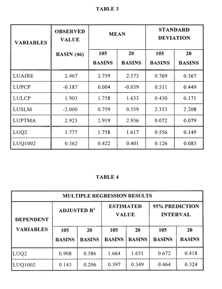
Tables 3 and 4 present respectively a companson of the means and standard deviations of aIl basin and flood variables and the results of the multiple regressions of the flood - on the basin variables, for the neighbourhoods of 105 and 20 basins. An examination of these statistics shows that the standard deviations of aIl basin and flood variables (except for the basin variable (PTMA) are smaller for the 20-basin neighbourhood than for the initial 105 basin neighbourhood. Although the adjusted squared
correlation coefficient R 2 of the basin variable LUQ2 is smaller for 20 basins th an for 105
basins, the corresponding prediction interval is smaller because of the smaller standard deviation of LUQ2 for this neighbourhood.
Thus, the 20-basin neighbourhood IS more satisfactory for estimating the flood
variables of the ungauged basin (46) because it is more homogeneous.
Figures 12 and 13 show the error vectors for the 20-basin neighbourhood in the
22 A canonical correlation approach to the detemlination of homogeneous regions for regional flood estimation
original units of the flood variables gives an intuitive picture of the performance of the canonical correlation method.
These two diagrams must be studied in detail to disco ver the reasons for the different lengths and directions of the error vectors for the different gauged basins of the neighbourhood.
Figure Il shows the geographical locations of the basins of the 20-basin neighbourhood. The fact that four basins of north-western Ontario are grouped with basins of south-western Ontario requires further hydrological analysis.
The most important features of the canonical correlation method are:
(1) Before proceeding to the estimation of the flood characteristics of the ungauged
basin, it inc1udes a detailed study of the re1ationships between the basin and the flood variables of the gauged basins to ensure that the latter variables can be estimated from the former.
(2) The homogeneous region used for the estimation is determined in the canonical
space of the flood variables which is based on the relationships between the basin and the flood variables.
The method of canonical correlation was compared to other current methods of delineation of homogeneous regions such as regions of influence (Zrinji and Bum 1994), correspondence analysis (Birikundavyi et al 1993), and L-moments (Gingras et al 1994), and was found to give better results for the basins considered in the study (GREHYS 1996b)].
Given n basins, p standardized basin-related variables xj and m standardized
flood-related variables qj (e.g. quantiles of a fitted probability distribution), where usual1y p~ m,
we compute the m canonical correlation coefficients r] ~ r2, ••• , ~ rm and the m pairs of
standardized basin - and flood-related canonical variables vj and wj respectively.
The flood-related canonical variables wj can be estimated from the corresponding
basin-related canonical variables vj using the simple regression equations:
W
j=
r
j v j(j =
1, 2,. . "m)
It must be noted that the flood variables (q], ... , qm) can be estimated usmg the
multiple regressions
ij
j =f
j(Xl"'"
xp)
or equivalently the multiple regressionsij
j=
f
j(v
1 " " , Vni) .
Thus the use of canonical variables results in a reduction of thedimensionality of the space of basin variables from p to m in a way that takes into account their relations with the flood variables. As a result, the number of flood variables that can be estimated is equal to the number of significant canonical correlation coefficients.
Statistical packages usually plot diagrams of (v]' w]), (v2, w2) etc., i.e. the pairs of
canonical variables having maximum correlation coefficients. Given the difficulties in
interpreting the canonical variables (e.g. Kendall and Stuart, 1968), it is preferable to plot
the uncorrelated pairs of canonical variables (v]' v2), (v]' v3) ••• (vj ' vk) etc., where j:;t:k
along with the corresponding scatter diagrams (w], w2) ••• (wj ' wk) of uncorrelated
flood-related canonical variables. The pairs of canonical variables (v]' v2) (w1, w2) etc.
respectively define the spaces of linearly transformed basin- and flood-related variables in which the points represent individual basins. If the basin variables are good predictors of
26 A canonical correlation approach to the detennination ofhomogeneous regions for regional flood estimation
the flood-related variables, the patterns of points in the corresponding scatter diagrams are similar.
It is useful to compute the structure correlation coefficients i.e. the correlation
coefficients between the original and the canonical variables which help to determine the contribution of each of the basin variables to the flood variables.
For large samples, the statistical significance of the set ofm cananical correlation coefficients can be tested by Bartlett's statistic:
v
=
-(n
-1-(p
+ 1 +m)/2
)i)n{l-
rf )
j=1
which, under the normality assumption, is distributed as chi-square with (pxm) degrees of freedom. If successive pairs of canonical variables are to be tested, the degrees of freedom must be modified. For example, the degrees of freedom associated with the second pair of canonical variables are (p-l) • (m-l) and so on.
The square of the canonical correlation, coefficient rj
2
is a measure of the shared
variance between the canonical variance vj and wj • Our main interest, however, is the
proportion of the variance of the flood variables accounted for by the basin variables. An
appropriate measure of this proportion is the redundancy index Rdq/v which is equal to the
mean of the proportions of the variances of the flood variables (ql , ... qrn) accounted for by
the canonical variables (VI"'" vrn) or equivalently by the basin variables (XI"'" xp)' The
where:
Rd
Xk
= contribution of the kthpair of canonical variables to the redundancy index Rd;/"
Rdqj( = contribution of the jth basin variable to the redundancy index Rd;/"
Given the estimated point \V (Z) = ~(Z) ... ~(Z) in the m-dimensional space of the
canonical variables and under the normality assumption, the (1-a) per cent confidence
region for the point is given by the equation:
where A is the (m x m) diagonal matrix of the squared canonical correlation coefficients
(r]2, ... ,
r;nJ
andMlw(i)-
w(z)
J
is the Mahalanobis distance of the point wei) from theestimated point \V(Z).
This confidence region can be interpreted as the (1-a) per cent neighbourhood of
the point \V(Z) (Ribeiro-Correa et al 1994). In the special case of m=2 the above equation is simplified:
M[w(i),
w(z)]
=[W](:)~r,~](Z)
+[W2(?~r.~2(Z):Ç
x2(a,2)
] 2
If the normality assumption is not valid, the Mahalanobis distance is a weighted
distance of the basin wei) from the estimated location V<Z) of the ungauged basin, with
a Significance level. Regression parâmeters.
ith distance oftwo points in the space (VI' •.. ' vrn ).
ith distance oftwo points in the space (wl,··., wrn ).
e Regression error.
LUAIRE loglo [Drainage are a (km2 )].
LULCP loglo [Length of main river channel (km)].
LUPCP loglo [Slope of main river channel (rn/km)].
LUSLM loglo (SLM + 0.01) where SLM = area of drainage basin controlled by lakes
and swamps (km2
)
LUPTMA loglo [Mean annual precipitation (mm)].
LUQ2 loglo [Annual maximum flood of2-year return period (m3
/sec)].
LUQI002 10glo [Ratio of the 100-year maximum flood to the 2-year maximum flood).
M(i) Mahalanobis distance of gauged basin (i) from the estimated point [w(i), 2.(Z)]
of the ungauged basin Z.
fi Number of flood variables.
n Number of basins.
p Number of basin variables.
ql'0oo, qrn Flood variables.
r l"'" r ru Canonical correlation coefficients.
30 A canonical corrclation approach to the determination of homogeneous regions for regional flood estimation
Rdq/v Redundancy index.
v i'" •• ' V m Canonical variables of the basin variables.
V Bartlett' s statistic.
W 1,···, Wm Canonical variables of the flood variables.
Acreman, M.C. and Wiltshire, S.E. (1989). The regions are dead: long live the regions. Methods of identifying and dispensing with regions for flood frequency analysis. IAHS Publ. no. 187,175-1988.
Andrews, F.M. and Inglehart, R.F. (1979). The structure of subjective weIl being in nine Western Societies. Social Indicators Research 6, 73-90.
Bates, B.C., Rahman, A., Mein, R.G. and Weinmann P.E. (1998). Climatic and physical factors that influence the homogeneity of regional floods in southeastern Australia, Water Resources Research 34 (12) 3369-3381.
Bernier, J. (1992). Modèle regional à deux nIveaux d'aléas. Interim Report NSERC Strategic Grant No STR 0118482, Il p.p.
Birikundavyi, S., Rousselle, J. and Nguyen, V.T.B. (1993). Determination des régions homogènes pour le Québec et l'Ontario: Une approche par l'analyse des corréspondances et la classification ascendante hierarchique. Rapport final, Subvention stratégique CRSNG, No STR 0118482, École Polytechnique de Montréal, p. 44.
Borg, I. and Lingoes, D. (1987). Multidimensional similarity structure analysis.
Springer-Verlag.
Burn, D.H. (1990a). An appraisal of the 'region of influence' approach to flood frequency analysis. Hydrological Sciences, Journal, 35 (2) 149-165.
Burn, D.H. (1990b). Evaluation of regional flood frequency analysis with a reglOn of influence approach. Water Resources Research 26 (10) 2257-2265.
32 A canonicat correlation approach to the determination ofhomogeneous regions for regional flood estimation
Cavadias, G.S. (1989). Regional flood estimation by canonical correlation. Paper presented to the 1989 Annual Conference of the Canadian Society of Civil Engineering, St. John's Newfoundland.
Cavadias, G.S. (1990). The canonical correlation approach to regional flood estimation. Regionalization in Hydrology. Proc. of the Ljubljana Symposium, IAHS. Publ. No. 191:171-178.
Cavadias, G.S. (1995). Regionalization and multivariate analysis: The canonical correlation approach. In "Statistical and Bayesian methods in hydrological sciences". IHP-V, Technical Documents in Hydrology No. 20, UNESCO, Paris.
Chowdhury, J.V., Stedinger J.R. and Lu, L.H. (1991). Goodness of fit test for regional generalized extreme value distributions. Water Resour. Res. 27(7), 1765-1776. Cooley, W.W. and Lohnes, P.R. Multivariate data analysis. Wiley 1971.
Cunnane, C. (1986). Review of statistical models for flood frequency estimation. Keynote paper in: International Symposium on Flood Frequency and Risk Analysis (Baton Rouge, May 1986). Reidel.
Dalrymple, T. (1960). Flood frequency analysis. USGS Water Supply Paper 1534 A., p. 60.
Dillon, W.E. and Goldstein, M. (1984). Multivariate Analysis, p. 139. John Wiley.
Dubes, R. and Zeng, G. (1987). A test for spatial homogeneity in cluster analysis. Classification 4, 33-56.
Dupuis, L. and Rasmussen, R.F. (1993). Évaluation de méthodes «indice de crue» pour l'estimation d'une distribution régionale. Rapport interne INRS-Eau, No 1-125, pp. 26.
Gingras D., Adamowski, K. and Pilon, P.J. (1994). Regional flood equations for the Provinces of Ontario and Quebec. Water Resour. Bull. 30(1), 55-67.
Gingras, D. and Adamowski, K. (1992). Coupling of nonparametric frequency and L-moment analysis for mixed distribution identification. Water Resour. Bulletin: 28(2), 263-272.
Gottschalk, L. (1985). Hydrological regionalization in Sweden. Hydrol. Sci. J. (30) (1).
Green, P .E. (1978). Analyzing multivariate data. The Dryden Press, Hinsdale, Illinois. GREHYS (1996a). Presentation and review of sorne methods of regional flood frequency
analysis. J. Hydrol. 186 (1-4), 63-84.
GREHYS (1996b). Intercomparison of flood frequency procedures for Canadian rivers. J. Hydrol. 186 (1-4), 85-103.
Hosking, J.R.M. and Wallis, J.R. (1993). Sorne statistics useful lU regional frequency
analysis. Water Resour. Res. 29(2),271-281.
Hotelling, H. (1936). Relations between two sets ofvariates. Biometrica28:321-377. Kendall, M.G. and Stuart, A. (1968). The advanced Theory of Statistics, Vol 3. 2nd ed.
Charles Griffin & Co. London.
Kuczera, G. (1982). Combining site-specific and regional information: an empirical Bayes' approach. Water Resour. Res. Vol. 8, No. 2, pp. 306-314.
Leutner, D. and Borg, 1. (1983). Zufallskritische Beurteilung der Übereinstimmung von
Factor und MDS-Konfigurationen. Diagnostica 29, 320-335.
Leutner, D. and Borg, 1. (1985). Zur Messung der Übereinstimmung von
multidimensionalen Konfigurationen mit Indizes. Zeischrift für Sozialpsychologie, 16,29-35.
34 A c,'monical correlation approach to the determination ofhomogeneous regions for regional flood estimation
Mosley, M.P. (1981). Delimitation of New Zealand hydrological regions. J. Hydrol. 49, 173-192.
Mosteller, F. and Tukey, J.W. (1977). Data Analysis and Regression. Addison-Wesley. Ouarda, T.B.M.J., and Ashkar, F. (1995). The peaks-over-threshold (POT) method for
regional flood frequency estimation. Proceedings of the 48th
Annual Conference of the Canadian Water Resources Association, Fredericton, N.B., Canada, 641-659. Ouarda, T.B.M.J., Haché, M. and Bobée, B. (1998). Regional estimation of extreme
hydrological events, INRS-Eau, Research Report No. R-534 (In French), Quebec, Canada, p. 181.
Ouarda, T.B.M.J., Haché, M., Bruneau, P. and Bobée, B.
(2000).
Regional floodpeak and volume estimation in Northern Canadian Basin, Journal of Cold Regions Engineering of the AS CE, 14(4): 176-191.
Panu, V.S., Smith, D.A. and Ambler, D.C. (1984). Regional flood frequency Analysis for the island of Newfoundland. Environment Canada and Department of Environment, Province of N ewfoundland.
Ribeiro-Correa, B., Cavadias, G.S., Clement, B. and Rouselle, J. (1994). Identification of hydrological neighborhoods using canonical correlation analysis. Journal of Hydrology 173 (1995) 71-89.
Rogers, A. (1974). Statistical Analysis of Spatial Dispersion. Pion Ltd.
Roy, R. (1993). Regionalisation de Caractéristiques de Crue, Utilisation d'une Méthode Combinant les Approches Déterministes et Stochastiques, Ph.D. Thesis, INRS-Eau. Stewart, D.K. and Love, W.A. (1968). A general canonical correlation index.
Torranin, P. (1972). Applicability of canonical correlation in hydrology. H.P. 58, Colorado State University, p. 30.
United States Water Resources Council (1977). Guidelines for Determining Flow Frequency. USWRC, 2120 Long Island NW, Washington, DC.
Wiltshire, S.E. (1986). Regional flood analysis II: multivariate classification of drainage basins in Britain. Hydrol. Sci. J. 31 (3).
Zrinji, Z. and Burn, D.H. (1994). Flood frequency analysis for ungauged sites us mg a region of influence approach. Journal of Hydrology 153, 1-21.
List of tables
Table 1: Structure correlation matrix (l05 basins).
Table 2: Structure correlation matrix (20 basins).
Table 3: Comparative statistics of the basin and flood variables for 105 and 20 basins.
38 A canonical correlation approach to the detemlination ofhomogeneous regions for regional flood estimation Vl V2 Wl W2 LUURE .9468 .0702 .9069 .0235 105) 105) 105) 105) .0000 .4767 .0000 .8120 LUPCP -.6049 .1822 -.5794 .0609 ( 105) 105) ( 105) lOS} .0000 .0629 .0000 .5368 LULCP .9188 -.1477 .8801 -.0494
lOS} . ( lOS) lOS} ( 105)
.0000 .1326 .0000 .6166 LUSLM .4482 -.2652 .4293 -.0887 lOS} ( 105) lOS} ( 105) .0000 .0062 .0000 .3681 LUJ?'I'MA -.3417 -.5216 -.3273 -.1745 ( 105) ( 105) ( 105) ( 105) .0004 .0000 .0007 .0751 LUQ2 .9549 -.0264 .9969 -.0788 105) ( 105) 105) ( 105) .0000 .7895 .0000 .4242 LUQ1002 -.2863 .3192 -.2989 .9543 ( 105) 105) ( 105) 105) .0031 .0009 .0019 .0000 TABLE 1 V1 V2 W1 W2 LUAIRE .2355 .0151 .2049 .0096 20) 20) 20) 20) .3175 .9496 .3861 .9678 LUPCP -.0486 .0734 -.0423 .0468 ( 20) 20) ( 20) 20) .8388 .7586 .8596 .8446 LULCP .1268 .4252 .1103 .2715 20) 20) 20) 20) .5944 .0616 .643·5 .2470 LUSLM -.5520 .4394 -.4803 .2806 ( 20) 20) ( 20) 20) .0116 .0525 .0321 .2308 LUPT:-lA .2021 .4849 .1759 .3096 20) 20) 20) 20) .3927 .0302 .4582 .1840 LUQ2 .789'; .2686 .9072 .4206 20) 20) .201 201 .0000 .2522 .0000 .064a LUQ1002 .12a9 -.6314 .1482 -.9890 20) ( 201 201 ( 20) .5879 .0028 .5329 .0000 TABLE 2
TABLE 3 OBSERVED STANDARD MEAN VALUE DEVIATION VARIABLES BASIN (46) 105 20 105 20 BASINS BASINS BASINS BASINS
LUAIRE 2.467 2.759 2.573 0.769 0.367 LUPCP -0.187 0.004 -0.039 0.511 0.449 LULCP 1.903 1.758 1.633 0.430 0.171 LUSLM -2.000 0.759 0.559 2.353 2.208 LUPTMA 2.923 2.919 2.936 0.072 0.079 LUQ2 1.777 1.758 1.617 0.556 0.149 LUQ1002 0.362 0.422 0.401 0.126 0.083 TABLE 4
MULTIPLE REGRESSION RESULTS
ADJUSTED R2 ESTIMATED 95% PREDICTION
VALUE INTERVAL DEPENDENT
VARIABLES 105 20 105 20 105 20
BASINS BASINS BASINS BASINS BASINS BASINS
LUQ2 0.908 0.586 1.664 1.651 0.672 0.418
List of figures Figure 1. Figure 2. Figure 3. Figure 4. Figure 5. Figure 6. Figure 7. Figure 8. Figure 9.
The basic concept of canonical correlation.
Scatter diagrams (VI' v2) and (wl, w2).
Error vector diagrams in the spaces (ml' W2) and (ql' q2)'
Map of Ontario gauging stations.
Scatter diagram (VI' v2) for 105 basins.
Scatter diagram (wl, w2) for 105 basins. Diagram of ordered Mahalanobis distances.
Means and standard deviations of the variables LUQ2 and LUQ1002 vs the number of stations in the neighborhood.
Estimated LUQ2 of the ungauged basin (46) with 95% prediction intervals vs the number of stations in the neighborhood.
Figure 10. Estimated LUQI002 of the ungauged basin (46) with 95% prediction intervals vs the number of stations in the neighborhood.
Figure 11. Map of Ontario with the gauglng stations of the 20-basin neighborhood.
Figure 12. Error vector diagram in the space (wl, w2) for the 20-basin neighborhood. Figure 13. Error vector diagram in the space (Q2, QI 002) for the 20-basin
42 A canonical correlation approach to the determination ofhomogeneous regions for regional flood estimation
•
•
(:M
• \:- :.:J
.... ,...
•
l
)
><
~[U
>
.
. . .... N . . . ~ ... + .. 4'., .. CX
0,...,... _ _ _ _ _ - - -... ... ... N ... " .... 41 ~ . . . . '~ ~ . . . C.
."
,;.i. /!Ilr•
-82 • S1•
--lin -Ba vt' \'2e_
e e -en.
.,
v1 es" FIG 2~
e82-0
-l
..
~
OBn!en
I:i.~" ês w1 FIG 3 eSz•
•...
w1 q2 0---•
~o -82..
,
/
ê..o-1
~â,
-lin lb".44 A canonical correlation approach to the determination of homogeneous regions for regional flood estimation
•
• CI..
H•
Ille·•
•
•
'..
•
•ill
•
•
•
•
••
•
•
•
•
•
E..
:.
~ 0 0 çt)3~---,~---.---.--~----r---~~-r---~ .136
2
:101 50 :s~8 ·821
67 .89o
·96]
-2
.16 -44-3
-4~---~---~---~---L---~---~-3
-2
-1
o
v1
FIG. 51
2
3
46 A canonical correlation approach to the deterrnination ofhomogeneous regions for regional flood estimation
:3
.
.
2.5
r- 63 se2t-
~o·105·
..2.15 '.1"5
1.5
.64 .Bl ,80 -62 ·85·
SOS ·fl11
~1 ,10(\ .'le4'W
.e1P
2 sl!6~1038-9S
e7-~
0.5
4Q:4 35' .29as
-34 ffi10 ~è 6 a2 -48 lo~ ..(~9 -:l.20
-6~e ,100 ·31} -52 .2G .82 . ~7 aS.aE! 3g·zio..g -9 .if(tl J31 118-0.5
-67 21·
.fi380 -51 t~ ;11l 13e-1
~-1"
-'111 .4 -137 ·15 55 .lê3 89 .!oh -9~·
,70 =18 J'3-1.5
·1i 112·
-se
-2 .7 .... 13lt4
-2
-3
-2
-1
0
1
2
:$
w1
PIG. 6;PLOT OF MAHALANOBIS DISTANCE VS ORDER OF BASIN 199 se se ... ,;: ... .. 413 ... -.•... ~ ... _._~. 213
... -..
~... !
... .
\.. :~;;
:\~I
... ~ ... _... . ... ~ .. 13 213 49 613 S9 lee 129 OROER OF BASIN FIG. 748 A canonical correlation approach to the determination ofhomogeneous regions for regional flood estimation .1..5
•••
e •• •• 3r··--·~I:~~fL~f-=r-~-l···
: : : !j ...
-.~
___
._.L ..••.•. -.-•••.•..
--! ...
----.i._._._ .... _ ....1 .. __ ...
J ... __ .. ___
!
1
1
JI l
I l
j ! ~ i 1i'
T--_·_·~_·-f--··l--··_··L_·---l·---l
j 1!
j
1
1
t· .. ··· ... ··· ..
·! .. ·· ..
···t·· .. ·· .. ··· .. · .. ··· ....t··· .... ··· .... ···-t .... ·· .. ·· .... · .. ·_ ....
1
.. ·_·_ ....
·--·-1
l
'
1
11
1
1
!
.
1
1
.
!
!
...., ... :. ... ·.· ... ·.···( ...• _ ... - ... -c. __ ... "_ .. ~ ... __ ... -<Oo •••• " ... _._,,_ . . . _ ... _ •••• _ . . . .t
1
MEANO~F
LUQ10h21
1--
+ f:. .1. ~ .. : , . : t
-1-·_··-l~::-~r~;~t-~~l~::~~·I~--i
i
+: . -.e·.::-è·-·-e._.-a·_··e·_,-a···-e···-e-e
iJ
~.-.- j ' . ! ~1
~.. i._ ... __ ....
S • D OF LUQlo..0·2 _~ .... i._ ... _ .... .J. ___ .. __ .. ____ -'j l : ; . l i
•
ae04.
e.
.1 • • .128HUM8ER OF STATIoNs IN THE NEIGH80RHOOO
2.2 2 1..8 1..6
:
:
!
:
:
r---rOO-i---!---r-o_o--ro--i
95% UPPER PREDICTION LIMIT
.. ; ... .
ESTIMATED LUQ2
. .~
j~
... ! ... ···· ....···t···~·/·t···
... . -t ...•••• ···f··· .. ··· *~ ~ .~ .. ... :. .. .'.··r···1"··:\:···\····~·~·~····~·~t~·~····;;~~·~·~;·~~~·+·~·;~~·;····-t··
.... * ...
"* ..
*
.
*
* ...
* ...
~...
*., ...
~...
* ... '
~ ··1···u···1·· .. ··· ..···r ... _
...
~...
u • • • uu···1···· .... ···,t··· .. e 2B 4B 6B 89 lee 129NUMBER OF BASINS IN THE NEIGHBORHOOO
50 A canonical correlation approach to the detcrmination ofhomogeneous regions for regional flood estimation a.s 0.S
T----·---r---r---;oo-o----r--o
--+
ESTIMATED LUQ1002···f···*.. .
0.4:---I:l-t-lo::~:l"'":~,,.---r
*
~:
i i ~ ~ ~95% LOWER PREDICTION ·LIMIT
~
"'+---1-0.2
o ··~···t···t···j···f···f···f··
o 20 40 S0 se "l.ee . l.2e
NUM8ER OF STATIONS IN THE NEIGH80RHOOO
•
104 • '(") ::; tu 101~
"'-•
I~
----...
~
"'Tl 9,
12~
Il'
•
,
11,
69 '/76 16 , • - 20"LI'
26•
33•
~_ ... 1 300 Km FIG. 11 01....
52 A canonical correlation approach to the determination ofhomogeneous regions for regional flood estimation ru :3 2 1. e -.1. -2 36 38 5·f 80 104 76 ; 16 3 3 ~ ~ ~ ~
1.--..
-.-L--..
-.1-.-~~-L
L ..J... .... :
I i i -2 -1 e .1. 2 3 w.t FIG. 123.5 3.2