Real-Time Scheduling for Energy Harvesting Sensors

HAL Id: hal-00691222

https://hal.archives-ouvertes.fr/hal-00691222

Submitted on 25 Apr 2012

HAL is a multi-disciplinary open access

archive for the deposit and dissemination of

sci-entific research documents, whether they are

pub-lished or not. The documents may come from

teaching and research institutions in France or

abroad, or from public or private research centers.

L’archive ouverte pluridisciplinaire HAL, est

destinée au dépôt et à la diffusion de documents

scientifiques de niveau recherche, publiés ou non,

émanant des établissements d’enseignement et de

recherche français ou étrangers, des laboratoires

publics ou privés.

Real-Time Scheduling for Energy Harvesting Sensors

Maryline Chetto, Hussein El Ghor, Rafic Hage Chehade

To cite this version:

Maryline Chetto, Hussein El Ghor, Rafic Hage Chehade. Real-Time Scheduling for Energy Harvesting

Sensors. The 6th International Conference for Internet Technology and Secured Transactions, Dec

2011, Abu Dhabi, United Arab Emirates. pp.396. �hal-00691222�

Real-Time Scheduling

for Energy Harvesting Sensors

Maryline Chetto

Hussein EL Ghor

Rafic Hage Chehade

Lebanese University

Institut Universitaire de Technologie - Saida E-mail: rafichagechehade@ul.edu.lb

Abstract— Energy harvesting is the conversion of ambient energy into electricity to power small devices such as wireless sensors, making them self-sufficient. The electrical energy used to power them is variable over time and limited by the capacity of the energy storage (battery or ultra-capacitor). In general, these embedded devices have to adhere to real-time constraints expressed in terms of deadlines. In this paper, we present power management and scheduling solutions for energy harvesting systems having real-time constraints such as most of wireless sensors. We show how to answer questions like the following: When should the system use energy? When should it be idle and recharge the energy storage? We review the main properties of a scheduler known as Earliest Deadline with Energy Guarantee (EDeg) and we report results of an experimental study.

I. INTRODUCTION

New powering methods, as an alternative to the current disposable battery, permit autonomous sensors to scavenge the energy in the environment. Environmental applications include forest fire detection, monitoring the level of air pol-lution and health applications like tele-monitoring of human physiological data. Numerous harvesting modalities have been demonstrated such as solar, vibrational, motion based, etc. The energy harvested from the environment can be stored in either batteries or ultra-capacitors. Batteries have a higher energy density and lower leakage, while ultra-capacitors have a higher round trip efficiency and offer higher endurance in terms of charge-discharge cycles.

Over the last decade, several energy sources have evolved from human and animal power to fossil fuels, nuclear, hydropower, wind, and solar energy [6]. Moreover, many alternative sources of energy are still being researched and tested. Technologies are continually being developed and enhanced to improve energy sources. In our work, we focus on the solar energy since it can be assumed constant on average in a long term perspective.

In a REH (Real-time Energy Harvesting) system, we have to make the best use of the available power and the goal of a scheduler is to assign the tasks (programs) to time slots such that all timing and power constraints are satisfied every time. We then say that the system operates in an energy neutral mode by consuming only as much energy as harvested [4].

In this paper, we will describe how to dynamically man-age power in a single processor REH system where tasks

are scheduled according to the famous preemptive dynamic priority policy, Earliest Deadline First (EDF).

The intuition behind the proposed scheme is to run tasks as long as the energy storage is sufficient to provide energy for all future occurring tasks, considering their timing and energy requirements and the replenishment rate of the storage unit. When this condition is not verified, the processor has to be idle so that the storage unit recharges as much as possible and as long as the system will be able to meet all the deadlines.

The rest of the paper is organized as follows: We first present the necessary background and related work in Section II. We outline the models in Section III and crucial concepts including the slack energy in Section IV. In Section V, we present EDeg scheduler. Section VI is concerned with experimental results. Finally, we conclude the paper in Section VII.

II. RELATEDWORK AND NECESSARY BACKGROUND

Researchers started to address power and scheduling issues in the last decade but most of them do not consider both rechargeability of the batteries and real-time constraints. In the work by Allavena et al. in [1], power scavenged by the energy source is constant and all tasks consume energy at a constant rate. Later in [5], Moser et al. propose LSA (Lazy scheduling Scheduling Algorithm) to optimally schedule tasks with deadlines, periodic or not. In that work, the total energy consumption of every task is directly connected to its execu-tion time through the constant power of the processing device. But in a real application, instantaneous power consumed by tasks may vary along time depending on circuitry and devices required by the tasks. Very recently, in [3], we relaxed the restrictive hypothesis that links together energy requirement and execution time of tasks. We presented an on-line schedul-ing scheme called EDeg. Under energy constraints, simply executing tasks according to the EDF rule, either as soon as possible (EDS) or as late as possible (EDL) may lead to violate some deadlines. EDeg is a variation of EDF that relies on two fundamental concepts, namely slack time and slack energy.

III. MODELS AND ASSUMPTIONS A. Application model

We consider here a set of independent periodic tasks that can be denoted as follows: τ = {τi, i = 1, . . . , n}. A

four-tuple (Ci, Ei, Di, Ti) is associated with each τi. In this

characterization, task τi makes its initial request at time 0

and its subsequent requests at times kTi, k = 1, 2, ... called

release times. The least common multiple of T1, T2, . . . , Tn

(called the hyperperiod) is denoted by TLCM. Each request of

τi requires a Worst Case Execution Time (WCET) of Citime

units and has a Worst Case Energy Consumption (WCEC) of Ei. We assume that the WCEC of a task has no relation with

its WCET.

A deadline for τioccurs Diunits after each request by which

task τi must have completed its execution. We assume that

0 < Ci≤ Di≤ Ti for each 1 ≤ i ≤ n.

Tasks are scheduled on a single processor system. Task set τ is said to be feasible if all tasks meet the deadlines. B. Energy model

We assume that ambient energy is harvested and converted into electrical power. We cannot control the energy source but we can predict the expected availability with a lower bound on the harvested source power output, namely Ps(t). This power

is then the instantaneous charging rate that incorporates all losses caused by power conversion and charging process. It is stored in a device with capacity C.

The stored energy at current time t is denoted as E(t). It can be measured with reasonable accuracy, used at any time later with no leak over time. We assume that energy production times can overlap with the consumption times.

IV. FUNDAMENTAL CONCEPTS

A. Slack time

The slack time of a hard deadline task set at current time t is the length of the longest interval starting at t during which the processor may be idle continuously while still satisfying all the timing constraints. Slack time analysis has been extensively investigated in real-time server systems in which aperiodic (or sporadic) tasks are jointly scheduled with periodic tasks [2]. In these systems, the purpose of slack time analysis is to improve the response time of aperiodic tasks or to increase their acceptance ratio. A means of determining the maximum amount of slack which may be stolen, without jeopardizing the hard timing constraints, is thus a key to the operation of the so-called slack-stealing algorithms. Determining slack time is realized at run-time by computing the so-called dynamic EDL(Earliest Deadline as Late as possible) schedule [2].

Illustrative Example:

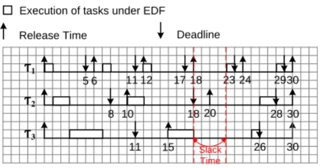
Consider a periodic task set Γ that is composed of three tasks, Γ = {τi| 1 ≤ i ≤ 3} and τi= (Ci, Di, Ti). Let τ1= (1, 5, 6),

τ2 = (2, 8, 10) and τ3 = (4, 11, 15). Before beginning to

schedule the task set Γ, we must verify the timing feasibility

Ƭ3 5 6 1112 1718 2324 2930 8 10 18 20 28 30 30 11 15 Slack 26 Time Execution of tasks under EDF

Release Time Deadline

Ƭ1 Ƭ2

Fig. 1. Computing Slack Time

condition. The processor utilization Up=P n i=0 Ci Ci = 19 30 ≤ 1,

consequently the necessary feasibility condition related to timing constraints, Up ≤ 1 is satisfied. Hence the total slack

time that can be used is equal to 11. We begin scheduling the task set Γ according to EDS until t = 8 where we have to insert a slack time.

To determine the slack time at time t = 18, we first compute the static EDL schedule for the interval [0, 30]. That means we have to compute the static deadline vector K and the static idle time vector D [2]. We

note that K = (0, 5, 8, 11, 17, 18, 23, 26, 28, 29) and

D = (3, 0, 0, 4, 0, 3, 0, 0, 0, 1).

Determining the slack time at time t = 18 is realized at run-time by computing the so-called dynamic EDL schedule precisely defined by the dynamic deadline vector K(t) and the dynamic idle time vector D(t) [2]. Figure 1 enables us to verify that K(t) = (18, 23, 26, 28, 29) and D(t) = (4, 2, 0, 0, 0, 1) and consequently the slack time is equal to 4. In what follows, we will use the idea of slack time to recharge the energy storage capacity whenever it is insufficient to execute more tasks.

B. Slack energy

On the other hand, slack energy is the maximum amount of energy that can be consumed from a given time t while still satisfying the timing and energy requirements of all the future occurring tasks. Slack energy must be computed by taking into account all periodic instances which have a deadline less than or equal to d, the deadline of the highest priority instance ready at current time t.

As total energy produced by the source within [t, d] is Rd

t Ps(t)dt, Slack energy(t) = E(t) +

Rd

t Ps(t)dt − A

where A is the energy demand required by the periodic task instances ready to be executed within the interval [t, d).

Illustrative Example:

Consider the above example. Now, we introduce the

energy consumption of tasks. Γ = {τi | 1 ≤ i ≤ 3} and

τi = (Ci, Di, Ti, Ei). Let τ1= (1, 5, 6, 12), τ2= (2, 8, 10, 15)

and τ3= (4, 11, 15, 22) (figure 2). We assume that the energy

storage capacity is C = 25 energy units at t = 0. For simplicity, we assume that the rechargeable power is constant

along time with (Ps= 5). Before beginning to schedule the

5 6 1112 1718 2324 2930 8 10 18 20 28 30 30 11 15 26 Execution of tasks under EDF

Release Time Deadline

T1 is released after t=10

and has deadline <18

Ƭ1

Ƭ2

Ƭ3

Fig. 2. Computing Slack Energy

task set Γ, we must verify the energy feasibility condition.

Ue=P n i=0 Ei Ci = 149 30 ≤ 5. Consequently, Ue≤ Ps.

Under EDeg, slack energy is computed whenever the highest priority task ready to be executed can be preempted by a task requiring energy. From time 0 until t = 10, tasks are executed according to EDS and the energy level is given by E(10) = 14 energy units. At t = 10 (figure 2), τ2 is the

highest priority task. Slack energy is then computed from all task instances released after t = 10 with deadline less than or equal to deadline of τ2 equal to 18.

Slack energy(10) = E(10)+ Z 18

10

Psdt−E1−E2= 22 (1)

Since slack energy is positive, τ2 can start execution while

still guaranteeing sufficient energy for all future occuring task instances.

V. THEEDeg ALGORITHM

We present hereafter a new scheduler based on the two previous concepts in order to enhance performance of classical EDF.

A. Presentation of the Algorithm

EDeg (Earliest Deadline with energy guarantee) runs tasks according to the earliest deadline first (EDF ). We consider that a task can consume energy with any power. This means that before executing a task, we must ensure that the energy storage is sufficient to execute this task during at least one time unit. When there is no sufficient energy in the storage unit, the processor has to remain idle so that the storage unit recharges entirely (E(t) = Emax) but making sure that there

is sufficient slack time.

Thus, the three major components of EDeg algorithm are E(t), Slack energy(t) and Slack time(t) where E(t) is the amount of energy that is currently stored at time t. P EN DIN G is a boolean which equals true whenever there is at least one task instance ready to be executed. Also, we define the function wait() to put the processor in the idle state and the function execute() to put the processor to run the ready job with the earliest deadline. The framework of the EDeg scheduling algorithm is as follows:

Algorithm 1 Earliest Deadline with energy guarantee algo-rithm (EDeg)

Input: A Set of Periodic Tasks τ = {τi|τi =

(Ci, Di, Ti, Ei) i = 1, · · · , n} According to EDF ,

current time t, battery with capacity ranging from Emax

to Emin, energy level of the battery E(t), source power Ps(t).

Output: EDeg Schedule. 1: while (1) do

2: while PENDING=true do

3: while (E(t) > Emin and Slack energy(t) > 0) do

4: execute()

5: end while

6: while (E(t) < Emax and Slack time(t) > 0) do

7: wait() 8: end while 9: end while 10: while PENDING=false do 11: wait() 12: end while 13: end while

From the EDeg algorithm, we notice the following: First, we never run out of storage, that means we always check for sufficient energy in the battery before executing any task instance. Second, the processor is only entered in the idle state when either the battery is empty or there is no more sufficient energy to guarantee the feasible execution of all future occurring tasks. Third, we recharge the battery to the maximum level when there is sufficient slack time. We only stop recharging when there is no more slack time or the battery is fully replenished. We can easily detect this condition by using an interrupt mechanism and adequate circuitry between storage unit and processing device. Finally, we only lose recharging power when there are no pending instances and the battery is fully recharged.

B. Efficiency

Complexity of an on-line algorithm is an evaluation of overheads that are produced when this algorithm actually runs. So, in a hard real-time context where all the tasks must imperatively meet their timing requirements, it is of more practical interest to make use of an algorithm which is both optimal in terms of scheduling performance and efficient in terms of computational complexity.

Under EDeg scheduling, overheads are mainly induced by computating the slack time and the slack energy. Slack time is computed solely when recharging the battery. Computing slack energy is realized when executing a periodic instance while other ones with earliest deadline will occur in the fu-ture. Consequently, complexity of computing the slack energy directly depends on the number of preemptions. Higher the number of preemptions, higher the overhead induced by the scheduler.

As shown in [2], the slack time of a periodic task set at a given time instant can be obtained on-line by computing the dynamic EDL schedule, with complexity O(K.n). n is the number of periodic tasks, and K is equal to dR_pe, where R and p are respectively the longest deadline and the shortest period of current ready tasks.

Moreover, the complexity for computing the slack energy is O(K.n). As EDeg has low and constant space requirements, this makes it easily implementable on many low-power, unso-phisticated hardware platforms including micro-controllers.

A suggestion to improve the efficiency of the scheduler in terms of overhead is to make some computations off-line. We can compute statically a lower bound on the slack time and a lower bound on the slack energy and use these approximation values at run time. The consequences will be only to stop charging earlier and to stop executing tasks earlier. And the number of tasks preemptions will increase while the processor overheads will decrease.

C. Illustrative Example

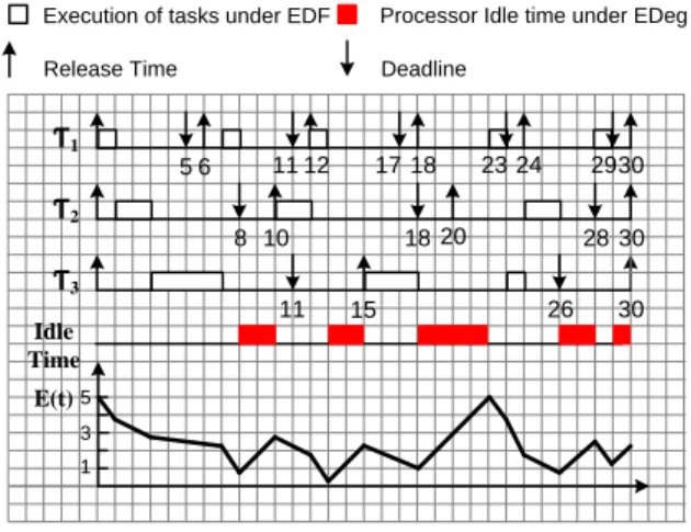
We consider the previous example. We note that Γ is not feasible if tasks are executed as soon as possible according to Earliest Deadline since the energy storage becomes empty at t = 18 (figure 3) where the system stops immediately. In

Ƭ3

5 6 1112 1718 2324 2930 8 10 18 20 28 30 30 11 15 26

Execution of tasks under EDF

Release Time Deadline

Idle Time

Processor Idle time under EDeg

Ƭ1

Ƭ2

E(t)5 3 1

Fig. 3. Task scheduling according to EDeg

details:

• According to EDeg, tasks of Γ are executed as soon as possible according to EDF until t = 15 where E(t) = 12 energy units.

• At t = 15, slack energy needs to be computed since

τ3 is the highest priority task ready to be executed with

future preemptions. As the slack energy is positive, τ3is

executed until t = 18 where there is no sufficient energy in the battery for execution. The processor is let inactive as long as the energy storage has not filled completely and the slack time is still positive.

• At t = 22, the battery is fully replenished (E(22) = 25)

energy units, τ1 is executed till t = 23, where E(t) = 18

energy units.

• At t = 23, τ3 completes its execution till t = 24 where

E(t) = 8 energy units.

• At t = 24, τ2has the highest priority and is executed till

t = 26, where E(t) = 3 energy units.

• Now, τ1 is ready and has the highest priority. As there

is no sufficient energy in the battery for execution, the processor is let idle for recharging till t = 28 where E(t) = 13 energy units.

• At time t = 28, τ1is executed till t = 29, where E(t) = 6

energy units.

• Finally, the processor is idle from t = 29 to t = 30 where E(t) = 11 energy units.

VI. EXPERIMENTAL RESULTS

A. Setup

We have implemented EDeg in a discrete event simulator in C/C++. To evaluate its effectiveness, we consider several task sets, each containing up to 30 randomly generated tasks. In this simulator, we implement EDeg with respect to EDS and two heuristics EDd 1 and EDd A. Where, EDd A is the Earliest Deadline as Soon as possible scheduler that discards ALL the ready instances whenever the storage unit is empty and consequently let the processor idle until the next release time and EDd 1 is the Earliest Deadline as Soon as possible scheduler that discards only one instance (the highest priority one) whenever the storage unit is empty and then let the processor idle until the next release time.

The rechargeable power Psis constant and we consider two

cases: low and high energy utilization. We assume that the energy storage is fully charged at the beginning of the sim-ulation. After a deadline violation is detected, the simulation terminates for EDL and EDS. Under EDd 1 and EDd A, the simulation continues until the end of the hyperperiod.

We compare the performance of the following techniques: (i) percentage of feasible task sets, (ii) average idle time and (iii) time overhead.

B. Low Energy Utilization

We first consider a system that consumes little energy relative to energy produced by the environment i.e. Ue/Ps=

0.3 where Ue=Pn_i=1 E_Ti

i.

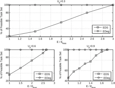
1) Percentage of Feasible Task Set: We experiment the

percentage of feasible task sets which are feasible with EDeg and not feasible with a greedy algorithm (EDS). We report the results of this simulation study where the processor utilization Up = {0.3, 0.6, 0.9}. Our simulation depicts the percentage

of feasible task sets over the energy storage E(t). For each task set, we compute Ef eas as the minimum storage capacity

which permits to achieve neutral operation i.e. all tasks are executed without violating deadlines and the battery is fully

recharged at the end of the hyperperiod. When Up = 0.3

(figure 4), all task sets are feasible under EDeg when the feasible energy Ef eas= 7100 energy units since EDeg will

benefit from the idle time to recharge the battery whenever the energy storage is insufficient to execute more tasks. On the other hand, EDS will need more energy storage than

1 1.2 1.4 1.6 1.8 2 2.2 2.4 2.6 2.8 3 20 40 60 80 100 E / E_feas

% of Feasible Task Set

U_p=0.3 1 1.5 2 2.5 3 20 40 60 80 100 E / E_feas

% of Feasible Task Set

U_p=0.6 1 1.2 1.4 1.6 1.8 40 60 80 100 E / E_feas

% of Feasible Task Set

U_p=0.9 EDS EDeg EDS EDeg EDS EDeg

Fig. 4. % of Feasible Task Sets for low energy utilization

EDeg to guarantee feasibility. In this case, all task sets are feasible under EDS when the energy storage is 21300 energy units. This means that EDeg can provide the same level of performance with a storage unit which is four times less.

When Up = 0.6 (figure 4), all task sets are feasible under

EDeg when the feasible energy Ef eas = 10800 energy

units. Under EDS, all task sets are feasible when the storage energy is about 28620 energy units,this means that the storage unit must be about 2.65 times bigger with EDS to maintain 100% feasible task sets compared to EDeg. We observe that, the relative performance gain of EDeg in terms of capacity savings is decreasing when the processor utilization rate is increasing.

For high processor utilization, the performance gain in ca-pacity savings decreases. This can be proved by our simulation since when Up= 0.9, EDeg obtains capacity savings of about

59% compared to EDS.

2) Average Idle Time: The schedule produced by any

scheduling algorithm can be characterized by the average duration of idle time intervals or the average number of idle time intervals in a given time window such as the hyperperiod of the schedule. Lower is the number of idle time intervals, lower will be the energy spent in transferring the processor from the inactive state to the active state. Let us note that new generation processors use dynamic power management (DPM) mechanisms. Using such mechanism can greatly enhance the performance of the system since it consists in putting off the processor whenever the processor has no task to execute. How-ever, this mechanism consumes energy and will be efficient as long as the processor remains inactive during a sufficiently long period.

In this section, we compute the total number of idle time intervals for EDeg, EDd A and EDd 1 by varying the processor utilization Up. In order to get an objective

measure-ment we take into account the percentage of deadlines being satisfied. Figure 5 gives a measurement of the total number

of idle time intervals weighted by the percentage of deadlines being satisfied. 0.1 0.2 0.3 0.4 0.5 0.6 0.7 0.8 0.9 1 0 0.05 0.1 0.15 0.2 0.25 0.3 0.35 U_p

Weighted Total Number of Idle Time Intervals

EDeg EDd_A EDd_1

Fig. 5. Idle time intervals for Low Energy Utilization

The total number of idle times in EDeg is lower than that of EDd A and EDd 1 since EDeg will benefit from the maximum time used to recharge the battery at the maximum level. As a result, the average idle time in EDeg will be greater than that of EDd A and EDd 1 and consequently the total number of idle times is smaller.

Consequently, short idle intervals that result in leakage are avoided with EDeg. And EDeg will have low energy overhead coming from transferring the processor from the inactive state to the active state.

3) Time Overhead: This experiment explores the time

overhead of EDeg i.e time spent to compute both slack energy and slack time. The objective is to prove that the gain in performance (from the above sections) is higher than the cost incurred by its implementation. Let us recall that EDF has no overhead (except due to preemptions and context switches) since no on-line computations are required. In the following, we measure the time overhead as the number of slack time and slack energy computations divided by the number of task instances. Under EDeg, for low values of Up, the time overhead is low (figure 6). As Up increases,

the time overhead increases. Nevertheless, it remains low even for Up = 0.9. Slack time computations are performed

whenever the processor needs to be idle because of no more energy. For low energy utilization, overhead to due slack time computations is consequently low. Slack energy computations are performed whenever a task is preempted by at least one higher priority task. Higher is Up, higher is the

number of task instances and so the number of preemptions and consequently higher is the overhead due to slack energy computations.

C. High Energy Utilization

Let us consider a system with high energy utilization i.e. Ue/Ps= 0.9. That means that the periodic task set consumes

0.1 0.2 0.3 0.4 0.5 0.6 0.7 0.8 0.9 0 0.01 0.02 0.03 0.04 0.05 0.06 U_p Time Overhead EDeg EDS

Fig. 6. Time Overhead for Low Energy Utilization

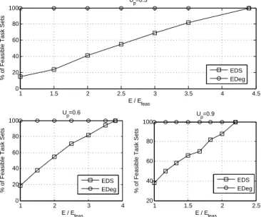
1) Percentage of Feasible Task Sets: As previously, for each task set, we compute Ef easas the minimum storage capacity

which permits to achieve neutral operation. Then we begin to increase Ef easuntil we reach 100% of feasible task sets with

EDS. When Up = 0.3 (figure 7), all task sets are feasible

1 1.5 2 2.5 3 3.5 4 4.5 0 20 40 60 80 100 E / E_feas

% of Feasible Task Sets

U_p=0.3 1 2 3 4 0 20 40 60 80 100 E / E_feas

% of Feasible Task Sets

U_p=0.6 1 1.5 2 2.5 20 40 60 80 100 E / E_feas

% of Feasible Task Sets

U_p=0.9 EDS EDeg EDS EDeg EDS EDeg

Fig. 7. % of Feasible Task Sets for high energy utilization

under EDeg when the feasible energy Ef eas= 10000 energy

units. This means that the feasible energy is increased by 29% relative to low energy utilization. This is because as the energy utilization increases, the consumed energy increases and consequently the minimum storage capacity which permits to achieve neutral operation Ef easincreases. On the other side,

all task sets are feasible under EDS when the energy storage is 44000 energy units. This means that EDeg can provide the same level of performance with a storage unit which is about 4.4 times less.

If we increase Up to 0.6 (figure 7), and run the simulation

again, we find that all task sets are feasible under EDeg when the feasible energy Ef eas= 15200 energy units. Under EDS,

all task sets are feasible when the storage energy is about 58000 energy units; that means that the storage unit must be

about 3.8 times bigger with EDS to maintain 100% feasible task sets compared to EDeg. We observe that, the relative performance gain of EDeg in terms of capacity savings is decreasing when the processor utilization rate is increasing.

For high processor utilization, the performance gain in ca-pacity savings decreases. This can be proved by our simulation

since when Up = 0.9, EDeg obtains capacity savings of

about 45% compared to EDS. That is because when the processor utilization is high, the processor rarely has chance to be idle to recharge the battery. This results in the decrease of performance gain of EDeg in terms of capacity savings.

When Up = 1, EDeg and EDS are the same since there is

no chance for EDeg to be idle to save energy.

As a conclusion, as the energy utilization increases, the consumed energy increases and as a result, the energy storage needed to achieve feasibility for EDeg increases. This is clearly shown in the simulation results since the feasible energy in high energy utilization is increased respectively by 29%, 28% and 25% for Up = 0.3, 0.6 and 0.9 when compared

to low energy utilization.

2) Average Idle Time: In this section, we present results of simulations performed to compute the weighted total number of idle time intervals for EDeg, EDd A and EDd 1 by varying the processor utilization Up from 0.1 to 1.

0.1 0.2 0.3 0.4 0.5 0.6 0.7 0.8 0.9 1 0 0.05 0.1 0.15 0.2 0.25 0.3 0.35 0.4 0.45 0.5 U_p

Weighted Total Number of Idle Time Intervals

EDeg EDd_A EDd_1

Fig. 8. Idle time intervals for High Energy Utilization

From figure 8, we can rapidly conclude that the total number of idle times in EDd 1 is greater than EDd A.

Depending on the concept of EDeg, when the energy storage is empty, the processor has to be idle so that the storage unit recharges to its maximum capacity or as much as possible and as long as the system will be able to meet all the deadlines. For this reason, the total number of idle time intervals must be smaller in EDeg than EDd A and EDd 1. Also, task instances are 100% feasible in EDeg and not in EDd A and EDd 1. Then, by dividing the total number of idle times over the percentage of feasible task instances, we will conclude that the weighted total number of idle time intervals in EDeg is lower than EDd A and EDd 1 by respectively 71% and 68%. Moreover, for high energy utilization, the consuming energy increases and the number of low battery level also increases. Thus, the number of idle times increases and consequently the average idle time decreases. This is proved by simulations

since the average idle time decreases by 45% from low to high energy utilization.

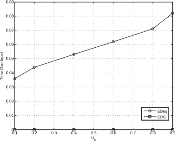
3) Time Overhead: For a realistic scenario, we must

take the time overhead into consideration. As stated above, there is no overhead under ED scheduling. In this ex-periment, we explore the time overhead by varying the processor utilization (Up). The chosen values for Up are

{0.1, 0.2, 0.4, 0.6, 0.8, 0.9}. 0.1 0.2 0.3 0.4 0.5 0.6 0.7 0.8 0.9 0 0.01 0.02 0.03 0.04 0.05 0.06 0.07 0.08 0.09 Up Time Overhead EDeg EDS

Fig. 9. Time Overhead for High Energy Utilization

As shown in figure 9, when processor utilization Up

in-creases the time overhead inin-creases till it reaches maximum value when Up = 0.9. It is important here to note that time

overhead at Up= 0.9 relative to the total number of feasible

instances is very low. This means that the gain in performance for EDeg is higher than the time overhead.

Moreover, under high energy utilization, the time overhead increases. This is because as energy utilization increases, the consumed energy increases and as a result the need to compute the slack time increases. Consequently, the time overhead increases. This is proved by simulations since the average time overhead in high energy utilization increases by about 47% relative to low energy utilization.

VII. CONCLUSIONS ANDFUTUREWORKS

In this paper, we presented a scheduler dedicated to embed-ded systems such as wireless sensors which harvest energy from the environment. We considered a uniprocessor system that execute periodic tasks that consume energy during their execution with possibly different instantaneous consumption powers. The crucial part of the so-called EDeg scheduling algorithm lies on two on-line functions called slack time and slack energy.

The simulation study reports the performance of EDeg, primarily measured by the percentage of feasible task instances i.e. percentage of task that meet their timing requirements expressed in terms of deadlines. The study shows that EDeg outperforms the classical and well known Earliest Deadline First scheduler. Moreover, we demonstrated that the overhead of EDeg remains acceptable which makes it a practicable scheduler.

REFERENCES

[1] A. Allavena and D. Mosse, Scheduling of frame-based embedded systems with rechargeable batteries, In Workshop on Power Management for

Real-time and Embedded systems(in conjunction with RTAS 2001), 2001.

[2] M. Silly-Chetto. The EDL Server for scheduling periodic and soft aperi-odic tasks with resource constraints. The Journal of Real-Time Systems, 17: 1-25, 1999.

[3] M. Chetto and H.El Ghor. Real-time Scheduling of periodic tasks in a monoprocessor system with rechargeable energy storage. In WIP

Proceedings of the 30th IEEE Real-Time Systems SymposiumDecember

2009.

[4] A. Kansal, J. Hsu. Harvesting aware power management for sensor networks, In IEEE Proceedings of Design Automation Conference, 2006. [5] C. Moser, D. Brunelli, L. Thiele, L. Benini. Real-time scheduling for energy harvesting sensor nodes, Real-Time Systems, Volume 37, Issue 3, Pages: 233 - 260, December 2007.

[6] S. Priya and D.-J. Inman. Energy Harvesting Technologies. Springer, New York (USA), 2009.