an author's https://oatao.univ-toulouse.fr/25253
https://doi.org/10.1016/j.ijsolstr.2019.12.014
Jaillon, Agathe and Jumel, Julien and Lachaud, Frédéric and Paroissien, Eric Mode I Cohesive Zone Model Parameters Identification and Comparison of Measurement Techniques based on uncertainty estimation. (2020) International Journal of Solids and Structures, 191-192. 577-587. ISSN 0020-7683
Mode I Cohesive Zone Model Parameters Identification and Comparison
of Measurement Techniques based on uncertainty estimation.
Agathe Jaillona, Julien Jumelb, Frédéric Lachauda, Eric Paroissiena
a: Institut Clément Ader (ICA), Université de Toulouse, CNRS-INSA-ISAE-Mines
Albi-UPS, UMR 53123 Rue Caroline Aigle, F-31400 Toulouse
b: I2M, Université de. Bordeaux, Arts et Métiers Paris Tech, CNRS, I2M, UMR 5295,
F-33400 Talence
Abstract
Adhesive bondline mechanical behaviour is frequently described with cohesive zone models
(CZM). For mode I loading condition these phenomenological laws simply represent the
evolution of the peel stress as a function of the two adherends relative displacement normal to
the joint. Generally, these laws are identified rather than really measured using experimental
data obtained from crack initiation and propagation experiments such as the Double
Cantilever Beam Test (DCB). The uncertainty on parameter estimation are generally not
indicated, as for a DCB test it is only the critical energy release rate that has the most
influence on the results. However, the uncertainties on the other parameters prevent the use of
the identified TSL for other mechanical tests where mode I solicitations are predominant. In
this article, the purpose is to evaluate the methodologies reliability for the assessment of
mode I CZM. To do so, several methods used to evaluate CZM parameters are compared in
terms parameter estimation reliability. Synthetic noisy data are considered for a χ² function
minimisation. Then, sensitivity calculations are performed to determine the estimated
parameters standard deviation. By applying this procedure on different type of synthetic
measurements (respectively P(), J(,), backface strain and DIC) the ability of these
different techniques to capture the best parameters for a chosen CZM shape can be rigorously
Keywords: DCB; Cohesive zone model; Chi-square; sensitivity; confidence interval;
Nomenclature
𝑎 = Parameters vector
𝑎0 = Initial crack tip length (mm)
C = Covariance matrix
𝑐𝑜𝑟𝑟 = Correlation matrix
Δ = Opening at loading point (mm) = Opening at crack tip (mm)
𝜀𝑠 = Adherend deformation measured by gauges (μdef)
𝐸 = Young’s modulus of the adherend(MPa)
𝐸𝑎 = Young’s modulus of the adhesive (MPa)
𝐺𝑎 = Shear modulus of the adhesive (MPa)
𝐺𝑐 = Critical energy release rate (N/mm)
𝐼 = Quadratic moment (𝑚4)
J = Integral J (N/mm)
k = Parameters’ index number
L = Bonded overlap length (mm)
𝑛𝑑 = Number of measured data
𝑛𝑝 = Number of parameters
P = Force (N)
𝜎 = Stress in the adhesive (MPa)
𝜎𝑚𝑎𝑥 = CZM Maximal stress (MPa)
𝜎𝑛𝑜𝑖𝑠𝑒 = Gaussian noise standard deviation
𝜎𝑌 = Standard deviation
θ = Rotation at loading point (rad) t = Adherend thickness (mm)
𝑡𝑎 = Adhesive bond thickness (mm)
𝑡𝑖 = Data index number
𝑣𝑝 = Displacement jump at propagation (μm)
w = adherend width (mm)
𝜒2 = Chi square function
𝑥 = abscissa along the overlap (mm)
𝑌 = Experimental data vector
𝑌̂ = Theoretical data vector
𝑌0 = Area under the TSL elastic part (N/mm)
Abbreviations
CI Confidence Interval
CZM Cohesive zone model
DCB Double cantilever beam
DIC Digital image correlation
FE Finite Element
Std Standard deviation
TS = Traction separation
1 Introduction
Adhesive bonding has gained growing interest in many fields in particular in the
transportation industry. Indeed, this joining technique is known to offer a very competitive
strength to mass ratio. It is very adequate for composite structure assembly and leads to
drastic reduction of the fasteners numbers. However, the reliability of bonded joints is
difficult to assess especially in the aeronautical sector where the certification procedure for
structural parts are very demanding. The variability on the bonded joint strength may be due
to strong sensitivity to any surface pollution, or uncontrolled ageing phenomena but is also a
consequence of inadequate mechanical testing protocols. Indeed, the bonded interface
behaviour is still mainly determined with standard procedure, the tensile test on single lap
joint specimen being the most common one. The test results are known to be dependent on
the test conditions such as the loading rate, but also on the specimen geometry (adherend and
adhesive thicknesses, overlap length) and not only on the interface properties.
These past years Cohesive Zone Model (CZM) were introduced to describe the interface
behaviour and simulate the joint behaviour. These phenomenological laws have been also
used to simulate delamination processes in laminates. They represent the cohesive stresses
versus interface relative displacement evolution and could be considered as more robust
models since they describe not only the interface elastic behaviour but also irreversible
phenomena such as damage and/or plasticity. They enable a refined evaluation of the
cohesive stresses distribution along the interface during monotonous loading of the joint.
These models have been studied extensively from a theoretical and numerical point of view
and many contributions have used them for failure load prediction of many different
materials [1] [2] [3]. Considering pure mode I loading condition, these models are
alternatively called traction separation laws (TSL). Their shapes and corresponding
behaviour (i.e. brittle, ductile). TS parameters are adjusted using iterative procedure so that a
good agreement is found between experimental data and theoretical value found with an
analytical [4] or numerical model [5] [6]. The data used for the identification are generally
simple applied load versus resulting displacement even if more sophisticated technique are
also described.
The use of CZM should improve the joint strength prediction through more precise
description of the interface mechanical behaviour. However, the prediction of both crack
initiation and propagation regime may still suffer from a lack of precision mainly because the
TSL shape is chosen empirically rather than really being measured. Previous contributions
have evidenced that the predicted mechanical response of the joint depends on the TSL shape
especially for ductile adhesives [7] [8] [9]. This is why an extensive work has been ongoing
for the development of specialized experimental techniques for measuring precisely the
interface separation law (i.e. cohesive stress versus displacement jump across the interface).
These new characterization protocols lead to the use of new specimen and loading systems
such as the DCB fixture developed by Sørensen et al. which enable the direct determination
of the TSL through the differentiation of the J-integral [10] [11]. This same technic is used by
Anderson et al. but the adhesive elongation is measured with interference patterns [12]. The
development of digital image correlation over the last decades has also given access to a
whole new range of mechanical response. As it is possible to monitor the adherends’
deflection and rotation throughout the entire test. Shen and Paulino then used a hybrid inverse
method based on finite element analysis and Digital Image Correlation (DIC) to determine
the TSL shape and associated parameters [13]. DIC was also used by Lelias et al as a direct
method to extract the CZM using the differentiation of displacement and rotation at crack tip
[14]. More systematic routine to identify CZM from DCB test with digital image correlation
deformation can also be measured using optical [17] or resistive [18] strain gauges. As it
enable a precise location of the crack tip but can also be used for the direct identification of
the CZM through the differentiation of the backface strain signal evolution [19]. Direct
inversion techniques have also been proposed for the CZM reconstruction from the
experimental data obtain with BSM and J() techniques. On the contrary inverse methods
should be used to analyse DIC and P() measurements [14]. In these cases, some
assumptions are made on the TSL shape which must be set arbitrary and which can lead to
errors on latter predictions [20]. Moreover, the incorrect estimation of the TSL parameters
can also lead to erroneous prediction when applied to other kind of mechanical tests that are
subjected to mode I or more complex solicitations (i.e. SLJ, DLJ, … ).
Then, this contribution aims at proposing a systematic procedure to evaluate the sensitivity of the four methods (P(), DIC, J(,), BSM) to evaluate a triangular TSL parameters such as interface stiffness, strength and fracture energy. A simple semi-analytical model of a DCB
experiment considering non-linear interface behaviour is used to generate synthetic
experimental data with known interface behaviour. Some Gaussian noise [21] is added to the
data then a Levenberg-Marquart algorithm is used to minimize an error function and identify
the triangular TSL parameters. The Confidence domains for the group of fitted parameters are
obtained at the end of the minimization procedure for all four measurement-techniques. They
can be used for the evaluation of the identification quality and the techniques’ comparison.
2 χ2 minimisation and confidence intervals theoretical background
Obtaining model parameters from a set of experimental data can be achieved with different
techniques. The most common technique consists in minimizing an error function which may
exhibit significantly non-linear behaviour. In the following, least square minimization is
𝜒2(𝑎) = ∑ [𝑌(𝑡𝑖) − 𝑌̂(𝑎, 𝑡𝑖) 𝜎𝑌(𝑡𝑖) ] 2 𝑛𝑑 𝑡𝑖=1 (eq 1)
In equation (eq 1) Y(𝑡𝑖), 𝑡𝑖={1,…, 𝑛𝑑} represent the 𝑛𝑑 measured data used to identify the 𝑎𝑘 k={1,…,p} parameters. 𝑌̂ are the corresponding theoretical data obtained with the model. In equation (eq 1), the terms in the sum are weighted by the measurement error on the
experimental data 𝜎𝑌. This function is minimized using steepest gradient technique such as
Levenberg-Marquart algorithm until the minimum 𝜒2value is found and the corresponding
optimum set of parameters is determined. The quality of the optimization process can then be
evaluated using the R²-value.
Once 𝑎, the optimal parameters’ vector is found, parameters confidence intervals can be
evaluated by analysing the 𝜒2 function evolution near the minima. Indeed, the small variation
of one or several parameters will lead to an increase of the 𝜒2 value, a steep increase meaning
a high sensibility to any parameter fluctuation and then high reliability of the identification
process. First, evaluation of the confidence interval is obtained by performing second order
Taylor expansion of the 𝜒2 function near the minima. This results in a simple quadratic
approximation of the error function given by:
𝛥𝜒2 = 𝛿𝑎 𝐶−1𝛿𝑎 (eq 2)
Where the covariance matrix is defined as
𝐶 = 𝜎𝑌 2(𝑆𝑆𝑇)−1 (eq 3) with S corresponding to sensitivity function:
𝑆 = [𝑆𝑘(𝑡𝑖)] =𝜕𝑌̂(𝑎, 𝑡𝑖)
𝜕𝑎𝑘 (eq 4)
Assuming the standard deviation, 𝜎𝑌 2, is constant for all data points (eq 5), it can be
𝜎𝑌2 =∑ (𝑌(𝑡𝑖) − 𝑌̂(𝑝, 𝑡𝑖)) 2 𝑛𝑑
𝑡𝑖=1
𝑛𝑑 − 𝑛𝑝 𝑖 ∈ [1: 𝑛𝑑] (eq 5) The confidence intervals on the identified parameters can be obtained from the analysis of the
𝜒2 function evolution near the minimum. Indeed, for a given reliability and number of degree
of freedom (nd - identified parameters) the variation ∆𝜒2 of the error function due to
parameters variation 𝛿𝑎 should be less than the value defined by 𝜒2 function values table.
From the asymptotic analysis and expression, these confidence intervals can be estimated
once the covariance matrix has been determined. The envelope of the confidence domain is
then represented by an ellipsoid, when three parameters are identified. Likewise, for two
parameters it is represented as an ellipse. However, the real shape of the confidence region
might be different if the minimization problem is highly nonlinear.
For visualisation and analysis purposes, it might be needed to reduce the number of
parameters used. As joint confidence regions are larger than individual intervals for the same
confidence. It is then possible to project the covariance matrix on a lesser dimension.
The confidence region analysis can also give information on the correlation of the
parameters. A correlation matrix can be determined using the covariance matrix [23]. It will
give access to a normalised estimation of the linear correlation between each pair of
parameters, diagonal parameters being equal to one.
𝑐𝑜𝑟𝑟(𝑖. 𝑗) = 𝐶(𝑖, 𝑗)
√𝐶(𝑖, 𝑖)√𝐶(𝑗, 𝑗) (𝑖, 𝑗) ∈ [1: 𝑛𝑝] (eq 6) Knowing the correlation between parameters is important as it gives indication on how
uncertainties on one parameter propagate to another.
Parameter estimation and confidence regions determination for a model require numerous
model calculation that can become quite time costly. In order to avoid too much calculation
time, it appeared wiser to implement an analytical model rather than using finite element (FE)
model. The purpose of this analytical model is to simulate the mechanical response that could
be measured during an experimental DCB test. That is to say that it needs to give access to all
the specimen mechanical response enabling the determination of the load, the opening at
loading point, the rotation at loading point, the adherends’ deformation along the overlap and the adherends’ rotation along the overlap. These responses can be determined with the mechanical fields computed during the crack propagation along the overlap for an adhesive
having a bilinear CZM.
3.1 Modelling of DCB test with nonlinear interface behaviour
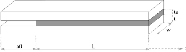
The DCB specimen, illustrated in Figure 1, is modelled as two Timoshenko beams having
rectangular cross section (width: w, thickness: t) and bonded with an adhesive layer whose
TS behaviour is represented with a bilinear TSL. The length of the bonded part is L. On the
right end of the specimen the two slabs are left unbounded over a distance equal to 𝑎0 and
considered as the initial crack length.
Figure 1: DCB specimen geometric data considered in the analytical model
The solving the local beam equilibrium enables the determination of the load displacement and J(θ,) curves during the whole test, as well as the shear forces, bending moment, adherends deflection and along the overlap. The whole analytical resolution methodology is
detailed in Jaillon et al. [20].
To illustrate the need for TSL identification techniques, some DCB test simulations are
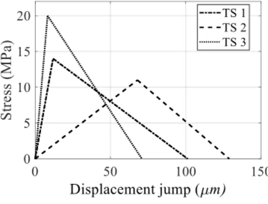
carried out for three bilinear TSLs. The DCB test specimen characteristics are presented
below considering triangular TSL which are defined by the adhesive effective modulus 𝐸𝑎,
the maximum stress 𝜎𝑚𝑎𝑥, and the critical energy release rate 𝐺𝑐. The chosen values are
summed up in Table 1.
Table 1: Traction separation laws parameters
Reference 𝑬𝒂 (MPa) 𝝈𝒎𝒂𝒙 (MPa) 𝑮𝒄 (𝑁/𝑚𝑚)
TS1 146 14 1.4178
TS2 20 11 1.4178
TS3 300 20 1.4178
These TSL can be displayed as stress function of displacement jump at crack tip, as Figure 2
illustrates it. In order to emphasize the importance of the TSL on the bonded specimen
mechanical response, these three laws will be used to compare the mechanical fields obtained
for each measurement method commonly used for DCB tests. Moreover, as this test is most
sensitive to the value of the critical energy rate, all three examples have the same one in order
to better visualize the differences due to the TSL parameters’ value only.
Figure 2: Three bilinear TSL.
3.2.1 TSL identification from the P(Δ) measurement technique
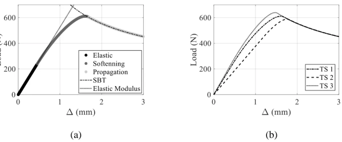
The first method proposed to evaluate TSL from DCB experiment is based on the analysis of
test [24], these data are systematically measured as it enables the evaluation of the interface
critical energy release rate which is based on compliance measurement evolution. As it can
be seen on Figure 3(a), P(Δ) curve is typically composed of three parts corresponding to the
CZM. The first one is linear. Then, once the adhesive begins to soften, the force keeps
increasing but nonlinearly and finally, when the critical energy release rate is reached crack
propagation begins.
(a) (b)
Figure 3: Load-displacement curves: (a) Division of the P(Δ) curve according to the TSL
phase; (b) Impact of the TSL on the P(Δ) response.
The responses from the three TSLs are presented in Figure 3(b) showing how the TSL may
affect the overall response of the specimen during testing. The TSL has an impact on the
phases previous to the crack propagation and it appears that it will affect the maximum force,
the opening displacement at crack propagation beginning and the nonlinearity of the peak.
Moreover, when the modulus is high, its impact become less significant and can be concealed
by the measurement noise.
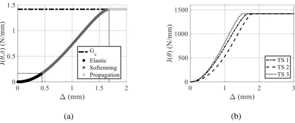
3.2.2 TSL identification from the J(,) measurement technique
The J integral evolution during the DCB test is obtained directly by measuring the specimen end rotation together with the applied load [25] [26]. The J(,) evolution reduces to three different regions, the elastic ad softening ones showing parabolic evolutions but with
propagation begins (Figure 4(a)). It appears that the TSL has an impact on the curvature of
the parabolas (Figure 4(b)). It also influences the opening value for which the energy release
rate becomes constant.
(a) (b)
Figure 4: Integral J function of the opening at loading point: (a) Division of the J(θ,δ) curve
according to the TSL phase; (b) Impact of the TSL on the J(θ,δ) response.
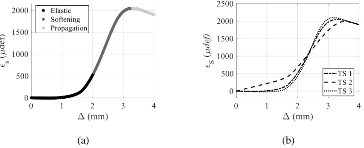
3.2.3 TSL identification from the Backface Strain measurement technique
Resistive gauges can be placed on the adherend’s upper face. The measurement of the slabs deformation, 𝜀𝑠, gives insight on the stress state of the adhesive bond directly underneath the
gauges using the relation:
𝜎 = −2 𝐸𝐼 𝑤𝑡
𝜕2𝜀 𝑠
𝜕𝑥2 (eq 7)
The gauges response is an indicator of the stress state of the adhesive below which phases are
given by Figure 5(a). It is worth noticing that the adherend deformation is maximal when the
crack tip is close to the gauge and that its value and curvature is influenced by the TSL as
(a) (b)
Figure 5: Gauges deformation function of the opening at loading point: (a) Division of the
Gauge curve according to the TSL phase; (b) Impact of the TSL on the Gauge response.
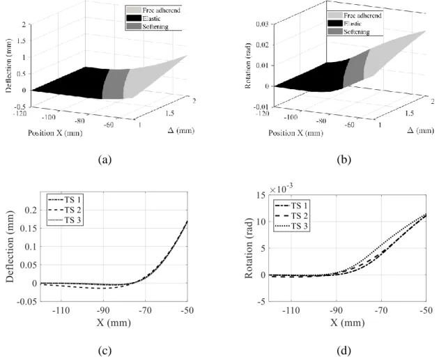
3.2.4 TSL identification from DIC measurement technique
During a DCB test digital image correlation (DIC) can be used to determine the deflection
and rotation of the adherends along the bonded area. Experimentally, this requires the use of
a speckle pattern and one or a couple of cameras. In the analytical model, the adherends
deflection and rotation of the neutral fibre are directly computed along the specimen without
generating any images of the adherends side. Moreover, in order to only investigate the
behaviour of the adhesive, the deflection and rotation of the adherend are analysed from the
crack tip abscissa X = -50 mm to X = 120 mm. The test is also only considered for an opening
at loading point included between Δ = 1 mm and Δ = 2 mm. Figure 6(a and b) highlights the
adhesive behaviour according to the CZM phase. It also enables the visualization of the crack
advances. The influence of the TSL is illustrated by Figure 6(c and d) for the deflection and
rotation of the adherends for Δ = 1 mm. The impact seems to be negligible and the
(a) (b)
(c) (d)
Figure 6: Digital image correlation results along the overlap during a DCB test: (a) Division
of the DIC – deflection curve according to the TSL phase; (b) Division of the DIC – rotation
curve according to the TSL phase; (c) Impact of the TSL on the deflection response; (d)
Impact of the TSL on the rotation response;
4 Confidence regions identification methodology
4.1 Material and geometric parameters
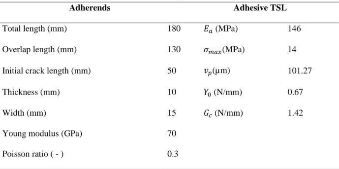
The analytic model, presented earlier, is used to simulate a DCB specimen. Its geometric and
material characteristics are summarized in Table 2. The adhesive, whose thickness is chosen
at 247µm, is implemented using a triangular cohesive zone model whose chosen parameters
of interests are arbitrarily chosen: the initial modulus the maximum stress and the
parameters and the associated critical energy release rate in mode I and surface area under the
elastic part, respectively 𝐺𝑐 and 𝑌0.
Table 2: DCB specimen geometric and material characteristics
Adherends Adhesive TSL
Total length (mm) 180 𝐸𝑎 (MPa) 146
Overlap length (mm) 130 𝜎𝑚𝑎𝑥(MPa) 14
Initial crack length (mm) 50 𝑣𝑝(µm) 101.27
Thickness (mm) 10 𝑌0 (N/mm) 0.67
Width (mm) 15 𝐺𝑐 (N/mm) 1.42
Young modulus (GPa) 70
Poisson ratio ( - ) 0.3
4.2 Synthetic experimental data generation
The analytical model is used to generate the nominal response of each mechanical field
previously described. In order to carry out the inverse identification and to estimate the
confidence intervals, a first approach is to generate synthetic experimental data by applying a
Gaussian noise. This noise enables the representation of experimental uncertainties that are
due to the measurement chain (i.e. load captors, gauges, DIC...). For each mechanical
response, a custom noise is generated as a normal distribution whose mean is equal to zero
and whose standard deviation is approximately 1% of the maximal mechanical response
(Table 3). Figure 7 displays the associated experimental data and optimisation results.
Table 3: Applied noise mean value for each mechanical response.
Method P(Δ) J(,) Gauges DIC - Deflection DIC - Rotation
Units N kJ/m² μdef mm rad
(a) (b)
(c) (d)
(e)
Figure 7: Synthetic measurements data with its optimization result; (a) P(Δ); (b) J(,); (c)
The minimization and confidence interval identification procedure were carried out for each
mechanical response that can be obtained on a DCB test. For clarity purpose, the process will
only be detailed for the force-displacement curve as it is similar for the other methods.
4.3 Application to the Force-displacement curve
The χ² minimization is executed on experimental data in order to determine the optimized
parameters triplet. To identify the confidence regions, sensitivity functions are determined
analytically using equation (eq 4). Mechanical responses are computed for a ±5% variation of
each parameters. The standard deviation (eq 5) between the optimized model data and the
experimental data are then computed enabling the determination of the covariance matrix. It
is possible to draw the confidence region in three-dimension, projected on 2-parameters plane
and projected in 1 dimension which gives access to confidence regions and intervals. The
confidence regions at 95% of the force-displacement curves are illustrated in Figure 8. The
ellipsoid and ellipses are centred on the nominal value. As expected, the individual
confidence intervals are smaller than the regions in two dimensions. It appears that the 95%
confidence intervals (i.e. individual) for the modulus is comprised between 127.3MPa and
164.7 MPa, for the maximal stress between [13.7, 14.5] MPa and for the displacement jump
between [98.2, 104.4] µm. Moreover, in order to assess the quality of the minimization and
confidence regions, the χ² optimization has been carried out 12 times for experimental data on
which were applied a new random noise. The results of these minimizations are illustrated in
Figure 8 as grey diamonds. It can be noticed that they are all included in the confidence
regions and intervals which is a quality assurance of the minimization procedure and shows
(a) (b)
(c) (d)
Figure 8: Confidence regions at 95% for the Force-displacement response: (a) confidence
ellipsoid; (b) confidence ellipse for 𝐸𝑎 and 𝜎𝑚𝑎𝑥; (c) confidence ellipse for 𝐸𝑎 and 𝑣𝑝; (b)
confidence ellipse for 𝜎𝑚𝑎𝑥 and 𝑣𝑝
The coupling between the parameters (i.e. 𝐸𝑎/𝜎𝑚𝑎𝑥, 𝐸𝑎/𝛿𝑝, 𝜎𝑚𝑎𝑥/𝛿𝑝) can also be obtained
with the correlation matrix (eq 6), in the force-displacement case it gives:
𝑐𝑜𝑟𝑟 = [
1 −0.51 0.50 −0.51 1 −0.99
0.5 −0.99 1
] (eq 8)
The correlation matrix indicates that the variation of the maximal stress and displacement
jump at propagation are so highly correlated that the variation of one can be quasi entirely
compensated by the other one, posing the problem of evaluation reliability. This implicates
eliminate this constraint, one could want to study the variation of critical energy release rate
instead of 𝑣𝑝 for instance.
Moreover, the confidence regions and interval should be analysed carefully as the methods
uses quadratic approximation when it is not necessarily true. Thus, the real confidence
regions might not be regular ellipses and confidence intervals in one dimension might not be
symmetric. However, this method enables the easy comparison of the different mechanical
responses that can be used to determine the adhesive traction separation law parameters.
5 Comparisons
The analysis procedure presented earlier has been applied to the other mechanical response as
well. From this study, an evaluation of the methods can be made from the comparison of the
confidence intervals, confidence regions and parameters coupling.
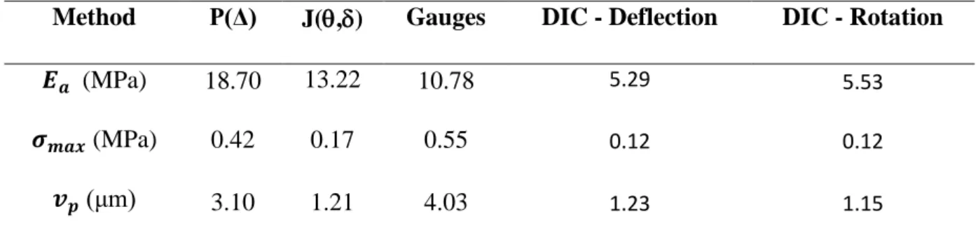
5.1 Confidence intervals and regions
The most straightforward results to analyse are the confidence intervals for each parameter
individually. They are symmetric and centred around the nominal value. Therefore, the
comparison between the methods will only be made with the interval radius. The results for
every method and every parameter for a 95% confidence interval are summarized in Table 4
Table 4: 95% confidence intervals comparison
Method P(Δ) J(,) Gauges DIC - Deflection DIC - Rotation
𝑬𝒂 (MPa) 18.70 13.22 10.78 5.29 5.53
𝝈𝒎𝒂𝒙 (MPa) 0.42 0.17 0.55 0.12 0.12
𝒗𝒑 (μm) 3.10 1.21 4.03 1.23 1.15
Overall, it appears that the results obtained using DIC are better than the other methods
especially for the determination of the initial modulus where the deflection confidence
dominates once again with radius of 0.12 MPa and 1.15 μm respectively. However, J(,) gives close results with CI radius of 0.17 MPa and 1.21 μm.
Another insight on the differences between the methods is given by the correlation matrix
(Table 5). Indeed, for each method parameters coupling appears to be different but follow the
same tendencies. The couple 𝜎𝑚𝑎𝑥/𝛿𝑝 appears to be strongly correlated for every methods.
This implies that during the minimisation their correct value might not have been found
accurately as a small variation of one compensate the deviation of the other. The two other
couples are moderately correlated. The use of DIC-deflection seems to ensure a low
correlation between the modulus and both 𝜎𝑚𝑎𝑥 and 𝛿𝑝.
Table 5: Correlation between the parameters couple
Method P(Δ) J(,) Gauges DIC - Deflection DIC - Rotation
𝑬𝒂/𝝈𝒎𝒂𝒙 -0.510 -0.639 -0.751 -0.149 -0.551
𝑬𝒂/𝜹𝒑 0.500 0.635 -0.747 0.160 0.476
𝝈𝒎𝒂𝒙/𝜹𝒑 -0.990 -0.996 -0.998 -0.980 -0.975
The visual analysis of the confidence ellipses given by the projection of the ellipsoid on two
dimensions planes gives complementary information (Figure 9). The smallest interval regions
are obtained for both DIC methods again.
(c)
Figure 9: Comparison of two-dimensions 95% interval regions comparison: (a) Modulus and
maximal stress plane; (b) Modulus and displacement jump at propagation plane; (c) Maximal
stress Modulus and displacement jump at propagation plane.
The ellipsoid volume analysis gives the overall confidence intervals as it reflects the tightness
of the confidence intervals in three dimensions. A small volume indicates a better estimation.
Table 6 shows that the DIC in rotation gives the smallest volume.
Table 6: 95% confidence ellipsoid volume
P(Δ) J(,) Gauge DIC - deflection DIC - rotation
Volume 35.71 2.06 11.74 1.86 1.52
5.2 TSL confidence envelop
From the three dimensions confidence volume, it is possible to determine the TSL that are on
the verge of the 95% confidence surface. Each parameter triplet, which is on the ellipsoid
surface, is used to generate the CZM envelope illustrated in Figure 10(a,c,e,g,i). From these
envelops the associated mechanical field envelop can be computed (Figure 10(b,d,f,h,j)). It
appears that even for the broader envelops the impact on the computed mechanical fields
seems to be negligible. That is to say that if the motivation of the CZM identification is only
results. However, if the TSL parameters are used to simulate the behaviour of other kind of
assemblies that can have a failure behaviour more sensitive to them than to 𝐺𝑐, then better
results will be obtained for DIC or J(,) methods as the parameters identified are closer to
the real nominal response.
(a) (b)
(c) (d)
(g) (h)
(i) (j)
Figure 10: Traction separation law envelope for 95% confidence regions: (a) P(Δ); (b) J(,);
(c) Gauges; (d) DIC – deflection; (e) DIC – rotation
Moreover, as the DCB test was designed to determine the critical energy release rate 𝐺𝑐 in
mode I, another verification can be done using its evaluation for the 95% confidence ellipsoid
surface. In Table 7, it appears that all methods except the gauges give a prediction with less
than 0.05% variation from the nominal value, which is equal to 1.41780 N/mm.
Table 7: Critical energy release rate evaluation for the 95% confidence volume
P(Δ) J(,) Gauge DIC - deflection DIC - rotation
𝑮𝒄,𝒎𝒐𝒚 1.41708 1.41766 1.41622 1.41773 1.41775
5.3 TSL application to a SLJ
In order to highlight the importance of the TSL parameter estimation, a semi analytical model
developed by Paroissien et al. has been used to simulate the force-versus displacement results
of a single-lap-joint test [14] [27]. The test geometry presented in Table 8 has been chosen in
order to obtain a failure caused predominantly by peeling rather than shear [28]. According to
Martin et al. for this test case, the mode mixity is simply managed by setting the same TS law
in mode II than in mode I. Moreover, the numerical results provided come from converged
model in terms of element density per characteristic length [29]. Table 8 presents the
geometric and material characteristics of the SLJ test.
To evaluate the impact of the TSL, the superior and inferior boundaries of the P(Δ) CZM
envelope were tested (Figure 11(a)). As illustrated in Figure 11(b), for a similar shear
behaviour but different TSL in mode I, the differences obtained are quite important. It
appears that there is a variation of 2000N in maximum load. This stresses out the importance
of a reliable estimation of the TSL parameters when carrying out the identification on a
different mechanical test.
Table 8: SLJ specimen geometric and material characteristics
Adherends Adhesive
Length outside the overlap (mm) 50 𝐺𝑎 (MPa) 50
Overlap length (mm) 50 𝑒𝑎(mm) 0.247
Initial crack length (mm) 50 𝐸𝑎𝑖𝑛𝑓 (MPa) 163
Thickness (mm) 10 𝜎𝑚𝑎𝑥𝑖𝑛𝑓 (MPa) 13.3
Width (mm) 25 𝐺𝑐𝑖𝑛𝑓 (N/mm) 1.4167
Poisson ratio ( - ) 0.3 𝜎𝑚𝑎𝑥𝑠𝑢𝑝(MPa) 14.7
𝐺𝑐𝑠𝑢𝑝 (N/mm) 1.4137
(a) (b)
Figure 11: (a) TSL envelope for the force-displacement; (b) Force versus displacement results
of a SLJ
Conclusion
The DCB test is widely used to identify the adhesive behaviour. However, the identification
of the correct TSL parameters from this test can be challenging because its mechanical
response appears not to be very sensitive. However, a reliable estimation of the mode I TSL
is needed when simulating other mechanical tests that are subjected to more complex
solicitations. A virtual test campaign has then been carried out in order to determine if one or
several of its mechanical fields enables a more accurate identification of the triangular TSL
parameter. To do so, the χ² minimization has been applied on synthetic experimental data. Its
analysis enables the identification of the parameters confidence domains, as well as their
coupling. It showed that in order to determine the parameters of an arbitrarily chosen TSL
shape (triangular) with an inverse method, the smallest confidence regions are given by
adherends’ rotation but the analysis of the deflection ensures a smaller coupling between the parameters. The slight augmentation of the confidence volume might be compensated by a
more accurate prediction of the parameters. This is to be expected has DIC gives access to
more data throughout the test. However, as the use of DIC needs a high investment in
equipment, the parameters can also be obtained using the J(,) method. It gives similarly
good results but its analysis needs to be done more carefully as its theoretical background is
limiting.
Acknowledgment
As part of the collaborative project S3PAC (FUI 21), this work was co-funded by BPI
References
[1] A. Cornec, I. Scheider and K.-H. Schwalbe, "On the practical application of the cohesive
model," Engineering fracture mechanics, vol. 70, pp. 1963-1987, 2003.
[2] J. Chen, "Predicting progressive delamination of stiffened fibre-composite panel and
repaired sandwich panel by decohesion models," Journal of Thermoplastic Composite
Materials, vol. 15, pp. 429-442, 2002.
[3] N. Chandra, H. Li, C. Shet and H. Ghonem, "Some issues in the application of cohesive
zone models for metal--ceramic interfaces," International Journal of Solids and
Structures, vol. 39, pp. 2827-2855, 2002.
[4] L. Škec, "Identification of parameters of a bi-linear cohesive-zone model using
analytical solutions for mode-I delamination," Engineering Fracture Mechanics, vol.
214, pp. 558-577, 2019.
[5] C. D. M. Liljedahl, A. D. Crocombe, M. A. Wahab and I. A. Ashcroft, "Modelling the
environmental degradation of adhesively bonded aluminium and composite joints using
a CZM approach," International Journal of Adhesion and Adhesives, vol. 27, pp.
505-518, 2007.
[6] M. S. Kafkalidis, M. D. Thouless, Q. D. Yang and S. M. Ward, "Deformation and
fracture of adhesive layers constrained by plastically-deforming adherends," Journal of
Adhesion Science and Technology, vol. 14, pp. 1593-1607, 2000.
[7] M. Alfano, F. Furgiuele, A. Leonardi, C. Maletta and G. H. Paulino, "Mode I fracture of
adhesive joints using tailored cohesive zone models," International journal of fracture,
vol. 157, pp. 193-204, 2009.
adhesive joints with cohesive zone models: effect of the cohesive law shape of the
adhesive layer," International Journal of Adhesion and Adhesives, vol. 44, pp. 48-56,
2013.
[9] S. H. Song, G. H. Paulino and W. G. Buttlar, "Influence of the cohesive zone model
shape parameter on asphalt concrete fracture behavior," in AIP Conference Proceedings,
2008.
[10] B. F. Sørensen, A. Horsewell, O. Jørgensen, A. N. Kumar and P. Engbæk, "Fracture
resistance measurement method for in situ observation of crack mechanisms," Journal of
the American Ceramic Society, vol. 81, pp. 661-669, 1998.
[11] B. F. Sørensen and T. K. Jacobsen, "Determination of cohesive laws by the J integral
approach," Engineering fracture mechanics, vol. 70, pp. 1841-1858, 2003.
[12] T. Andersson and U. Stigh, "The stress--elongation relation for an adhesive layer loaded
in peel using equilibrium of energetic forces," International Journal of Solids and
Structures, vol. 41, pp. 413-434, 2004.
[13] B. Shen and G. H. Paulino, "Direct extraction of cohesive fracture properties from
digital image correlation: a hybrid inverse technique," Experimental Mechanics, vol. 51,
pp. 143-163, 2011.
[14] G. Lelias, E. Paroissien, F. Lachaud, J. Morlier, S. Schwartz and C. Gavoille, "An
extended semi-analytical formulation for fast and reliable mode I/II stress analysis of
adhesively bonded joints," International Journal of Solids and Structures, vol. 62, pp.
18-38, 2015.
[15] M. Alfano, G. Lubineau and G. H. Paulino, "Global sensitivity analysis in the
identification of cohesive models using full-field kinematic data," International Journal
[16] B. Blaysat, J. P. M. Hoefnagels, G. Lubineau, M. Alfano and M. G. D. Geers, "Interface
debonding characterization by image correlation integrated with double cantilever beam
kinematics," International Journal of Solids and Structures, vol. 55, pp. 79-91, 2015.
[17] D. Sans, J. Renart, J. Costa, N. Gascons and J. A. Mayugo, "Assessment of the influence
of the crack monitoring method in interlaminar fatigue tests using fiber Bragg grating
sensors," Composites Science and Technology, vol. 84, pp. 44-50, 2013.
[18] J. Jumel, M. K. Budzik, N. B. Salem and M. E. R. Shanahan, "Instrumented End
Notched Flexure--Crack propagation and process zone monitoring. Part I: Modelling and
analysis," International Journal of Solids and Structures, vol. 50, pp. 297-309, 2013.
[19] J. Jumel, N. B. Salem, M. K. Budzik and M. E. R. Shanahan, "Measurement of interface
cohesive stresses and strains evolutions with combined mixed mode crack propagation
test and Backface Strain Monitoring measurements," International Journal of Solids and
Structures, vol. 52, pp. 33-44, 2015.
[20] A. Jaillon, J. Jumel, E. Paroissine and F. Lachaud, "Mode I Cohesive Zone Model
Parameters Identification and Comparison of Measurement Techniques for Robustness
to the Law Shape Evaluation," Journal of adhesion, p. Accepted, 2019.
[21] H. Haddadi and S. Belhabib, "Use of rigid-body motion for the investigation and
estimation of the measurement errors related to digital image correlation technique,"
Optics and Lasers in Engineering, vol. 46, pp. 185-196, 2008.
[22] S. Marsili-Libelli, S. Guerrizio and N. Checchi, "Confidence regions of estimated
parameters for ecological systems," Ecological Modelling, vol. 165, pp. 127-146, 2003.
[23] S. Hartmann and R. R. Gilbert, "Identifiability of material parameters in solid
mechanics," Archive of Applied Mechanics, vol. 88, pp. 3-26, 2018.
Applied Polymer Science, vol. 10, pp. 1351-1371, 1966.
[25] J. D. Gunderson, J. F. Brueck and A. J. Paris, "Alternative test method for interlaminar
fracture toughness of composites," International Journal of Fracture, vol. 143, pp.
273-276, 2007.
[26] T. Andersson and A. Biel, "On the effective constitutive properties of a thin adhesive
layer loaded in peel," International Journal of Fracture, vol. 141, pp. 227-246, 2006.
[27] E. Paroissien, F. Lachaud, F. M. da Silva and Lucas and S. Seddiki, "A comparison
between macro-element and finite element solutions for the stress analysis of
functionally graded single-lap joints," Composite Structures, vol. 215, pp. 331-350,
2019.
[28] L. J. Hart-Smith, "Adhesive-Bonded Single-Lap Joints.[analytical solutions for static
load carrying capacity]," 1973.
[29] E. Martin, T. Vandellos, D. Leguillon and N. Carrère, "Initiation of edge debonding:
coupled criterion versus cohesive zone model," International Journal of Fracture, vol.