HAL Id: hal-02882350
https://hal.archives-ouvertes.fr/hal-02882350
Submitted on 26 Jun 2020HAL is a multi-disciplinary open access archive for the deposit and dissemination of sci-entific research documents, whether they are pub-lished or not. The documents may come from teaching and research institutions in France or abroad, or from public or private research centers.
L’archive ouverte pluridisciplinaire HAL, est destinée au dépôt et à la diffusion de documents scientifiques de niveau recherche, publiés ou non, émanant des établissements d’enseignement et de recherche français ou étrangers, des laboratoires publics ou privés.
Mode I cohesive zone model parameters identification
and comparison of measurement techniques for
robustness to the law shape evaluation
Agathe Jaillon, Julien Jumel, Frederic Lachaud, Eric Paroissien
To cite this version:
Agathe Jaillon, Julien Jumel, Frederic Lachaud, Eric Paroissien. Mode I cohesive zone model parameters identification and comparison of measurement techniques for robustness to the law shape evaluation. Journal of Adhesion, Taylor & Francis, 2020, 96 (1-4), pp.272-299. �10.1080/00218464.2019.1669450�. �hal-02882350�
Mode I cohesive zone model parameters identification and
comparison of measurement techniques for robustness to the
law shape evaluation
Agathe Jaillona, Julien Jumelb, Frédéric Lachauda, Éric Paroissiena
a : Institut Clément Ader (ICA), Université de Toulouse,CNRS-INSA-ISAE-Mines Albi-UPS, UMR 53123 Rue Caroline Aigle, F-31400 Toulouse
b : I2M, Université de. Bordeaux, Arts et Métiers Paris Tech, CNRS, I2M, UMR 5295, F-33400 Talence
1 Abstract
Adhesive bonding modelling is often realised using cohesive zone models (CZM). For pure mode I loading, these laws represent the cohesive stress versus the interface displacement evolution designated as traction-separation laws (TSL). They enable the description of the interface irreversible phenomena such as damage and/or plasticity, while permitting a refined evaluation of the cohesive stress along the overlap. However, these laws are usually chosen a priori. For brittle and ductile adhesives the TSL shapes usually chosen are respectively bilinear softening and elasto-plastic. But the development of direct CZM measurements has highlighted that the law shapes can be more complex. The wrong initial choice of the TSL shape can then have an impact on the simulation results reliability. In this article, several methods used to evaluate CZM parameters are compared in terms of TSL shape robustness. Synthetic noisy data generated from a trapezoidal CZM are used for the inverse identification of a bilinear softening TSL. By applying this procedure on different type of synthetic measurements (respectively Force-displacement, J-integral, backface strain and DIC) the ability of these techniques to capture parameters for a chosen CZM shape that is not the right one enables a rigorous evaluation the robustness to the law shape.
Keywords: Cohesive zone models, Robustness, Mechanical properties of adhesives, Analytical models, Peel, Statistical analysis.
2 Introduction
Adhesive bonding is becoming an assembly technique appealing for the transport sectors especially for the aeronautic. As the need for a drastic reduction of the structures weight has led to a reassessment of the materials repartition and junction strategies. This positions the adhesive bonding as a viable competitor to the traditional bolting and riveting technics. As it has the capacity to assemble different materials such as metals and composites while needing less industrial stages and still retaining a competitive strength-to-mass ratio. However, the aeronautical sector is very demanding and severe for the qualification of the process. Yet, testing protocols currently used such as the single lap joint are also introducing variability in the adhesive strength. As they are not only dependent on the adhesive interface properties but also on the test conditions (i.e. loading rate) as well as the specimen geometry such as adherends and adhesive thickness and overlap length. This raises the issue on the validity of the testing protocols and then the reliability of the parameters determined which are used in numerical simulations.
The modelling of adhesive bonding is most of the time realised using cohesive zone models (CZM). They were first developed by Barenblatt [1] and Dugdale [2] and are used to describe the interface behaviour. These phenomenological laws were used intensively for a wide range of materials such as concrete [3], metals and especially for the simulation of delamination process in composite laminates [4, 5]. These laws represent the cohesive stress versus the interface relative displacement evolution and have the advantage to enable the description of the interface irreversible phenomena such as damage and/or plasticity, while permitting a refined evaluation of the cohesive stress along the overlap during monotonous loading. It can
also be used in more advanced models in order to describe the joint behaviour in fatigue [6, 7], creep or aging damage [8].
These models are extensively used in the literature in their theoretical and numerical aspects and many contributions have used then for pure mode as well as more complex loading solicitations [9]. For pure mode I loading, also known as peel solicitation, the cohesive zone models can also be designated as traction-separation (TS) laws. Their shape and corresponding parameters are usually determined empirically according to the expected behaviour of the adhesive. Indeed, it is widespread to use a bilinear softening (i.e. triangular) law shape for brittle adhesive and an elasto-plastic (i.e. trapezoidal) shape for ductile adhesive. Other law shapes has also been developed such as polynomial, exponential [10] or more sophisticated shapes such as polynomial [11] or interpolation based CZM [12]. The parameters are then identified using an iterative inverse identification method to obtain a good agreement between experimental data and analytical [13] or numerical model [14–16].
Many contributions have been made on the influence of the TS law shape on the predicted value for different specimen geometries and materials. For instance Song et al. showed that CZM softening shape influences numerical results considerably in the case of asphalt concrete disk-shaped compact tension test [17]. Similar results were obtained for butt-joints in shear [18], block peel tests [19] and thick DCB [20]. Moreover it was showed by Campilho et al. that the law shape also has an impact in SLJ test, especially for small overlap length [21, 22] and when the adhesive is highly ductile [23]. On the other hand, it appears that the DCB specimen with slim adherends is less sensitive to the TS law shape. Its global behaviour is mostly impacted by the critical energy release rate Gc [24]. However, as it was concluded by
Chandra et al., the appropriate TS law shape is needed in order to correctly describe the inelastic micromechanical process and thus to obtain meaningful simulation results [25].
This is why many studies are now investigating the direct measurement of the CZM properties. The most widespread technic, initially developed by Sorensen et al. [26] in mode II testing, consists in the differentiation of the integral J [27]. This same method has been implemented for pure mode I testing [18-30] and can be carried out with the measurement of the adhesive elongation at crack tip. The development of digital image correlation (DIC) has also brought out a new range of measurable mechanical data such as the adherends deflection and rotation along the overlap which can also be used to measure the CZM. However, the direct determination of the TS law leads to the identification of very complex law shapes [31; 32] that needs extensive data reduction scheme and that can then be difficult to implement and costly in computational time.
An alternative to the direct method to identify the correct law shape would be to find an inverse identification method that is robust to the law shape. That is to say that the parameters resulting from the minimisation would only give coherent results if the correct law shape has been implemented a priori. As a first step toward this direction, this contribution aims at determining if the application of the inverse method on five different DCB mechanical responses can give robust results. It is chosen to investigate the force versus displacement (P(Δ)), the energy release rate versus displacement (J(θ,Δ)), the adherends deformation with the use of gauges and the deflection and rotation of the whole adherends using DIC. For each of these mechanical responses a numerical test campaign has been carried out. In order to reduce calculation time, an analytical model is used to simulate a DCB test and its mechanical fields. Synthetic experimental data are generated using a trapezoidal CZM. The inverse method is applied on it with a bilinear softening TS law. The robustness to the law shape can then be evaluated for each mechanical response.
3 Modelling of DCB test with nonlinear interface behaviour
Parameter estimation and robustness to the law shape determination for a model require numerous model calculation that can become quite time costly. In order to avoid too much calculation time, it appeared wiser to implement an analytical model rather than using finite element (FE) model that can quickly become time consuming in pre and post processing as well. The purpose of this analytical model is to simulate the mechanical response that could be measured during an experimental DCB test. That is to say that it needs to give access to all the specimen mechanical response enabling the determination of the load, the opening at loading point, the rotation at loading point, the adherends’ deformation along the overlap and the adherends’ rotation along the overlap. These responses can be determined with the mechanical fields computed during the crack propagation along the overlap for an adhesive having a bilinear softening or a trapezoidal CZM. Their calculation methodology is detailed below and validated by comparing calculation with more complete simulation using the macro-element technique in Appendix I.
3.1 Model definition
An analytical model of a DCB specimen has been developed considering adherends modelled as Timoshenko beams. The specimen geometrical properties are represented in Figure 1. The adherends are considered to have a rectangular cross section (width: w, thickness: t). They are bonded over a length L and the initial crack tip where the adherends are left unbonded has a length equal to a. The adhesive has a nonlinear behaviour, either bilinear softening or trapezoidal. The adhesive layer has a thickness corresponding to ta.
Figure 1: DCB specimen geometrical data considered in the analytical model
The specimen adherends are chosen to have the same material properties leading to a symmetric specimen. The loading conditions are also symmetric as it is applied on the upper and lower adherend extremities and with opposite sign. These conditions permit to only consider the upper adherend and the half adhesive thickness for the solving of the local beam equilibrium along the overlap, 𝑥:
𝑑𝑀(𝑥)
𝑑𝑥 + 𝑇(𝑥) = 0 (eq 1)
𝑑𝑇(𝑥)
𝑑𝑥 − 𝑤𝜎(𝑥) = 0 (eq 2)
Where M, T and 𝜎 respectively corresponds to the local bending moment, the shear force and the local peel stress.
Timoshenko beam formulation leads to the following constitutive equations:
𝑀(𝑥) = 𝐸𝐼𝑑𝜑(𝑥)
𝑑𝑥 (eq 3)
(𝑥) = 𝜅𝐺𝑆 (𝑑𝑣(𝑥)
𝑑𝑥 − 𝜑(𝑥)) (eq 4)
material parameters E and G are respectively the Young’s modulus and the shear modulus. 𝑆 = 𝑤𝑡 corresponds to the beam cross section area. In case of a rectangular cross section the quadratic moment is computed as 𝐼 =𝑤𝑡3
12 and the shear correction coefficient is
approximately 𝜅 =5
6. By combining (eq 1) to (eq 4), the following equation is found:
𝑑4𝑣(𝑥) 𝑑𝑥4 − 1 𝜅𝐺𝑆 𝑑2𝜎(𝑥) 𝑑𝑥2 + 𝜎(𝑥) 𝐸𝐼 = 0 (eq 5)
The solution of this differential equation depends on the adhesive behaviour. In the present case, it will be solved for two nonlinear behaviour, bilinear softening and trapezoidal. As illustrated in Figure 2, both behaviours can be divided in two parts. The first one corresponds to an elastic behaviour and is identical for both. The second one is either a linear softening or a plastic behaviour. Thus, the differential equation will be solved for those three evolutions separately.
Figure 2: Nonlinear traction-separation law: bilinear softening and perfectly plastic
3.2 Elastic behaviour
𝜎 = 2𝐸𝑎 ∗ 𝑡𝑎 𝑣(𝑥) 𝑣 < 𝑡𝑎 𝜀𝑒 2 (eq 6)
Where 𝐸𝑎 ∗ corresponds to the apparent Young’s Modulus of the adhesive. The differential
equation (eq 5) which governs the evolution of the peel stress in the elastic regions then reduces to: 𝑑4𝜎(𝑥) 𝑑𝑥4 − 𝑘𝑒 𝜅𝐺𝑆 𝑑2𝜎(𝑥) 𝑑𝑥2 + 𝑘𝑒 𝐸𝐼𝜎(𝑥) = 0 (eq 7)
With the tangent stiffness in the elastic bondline region given by:
𝑘𝑒 = 𝑤2𝐸𝑎
∗
𝑡𝑎 (eq 8)
The general expression for the peel stress evolution in the elastic region along the bondline can then be expressed as:
𝜎(𝑥) = ∑ 𝐴𝑖𝑒𝜆𝑒,𝑖𝑥+ 𝐵 𝑖𝑒−𝜆𝑒,𝑖(𝐿−𝑥) 2 𝑖=1 (eq 9) with 𝜆𝑒,𝑖 = 𝜆𝑒√𝜀𝑒± √𝜀𝑒2− 1 = 𝜆𝑒𝛼𝑖 i ∈ [1, 2] (eq 10) where 𝜆𝑒 =1 4𝑘𝑒EI (eq 11) and
𝜀𝑒= √𝑘𝑒𝐸𝐼
2𝜅𝐺𝑆 (eq 12)
The 𝐴𝑖 and 𝐵𝑖 are constants determined .using the boundary and continuity conditions. The
other cohesive forces in the elastic region can then be obtained by integrating (eq 1) to (eq 4) and using the following boundary conditions:
𝑀(𝑥 = 0) = 𝑎𝑃 (eq 13)
𝑇(𝑥 = 0) = 𝑃 (eq 14)
3.3 Bilinear softening behaviour
The linear softening region is solved similarly as the elastic one. Its traction-separation equation is defined as:
= 𝜎𝑚𝑎𝑥 𝑣𝑒− 𝑣𝑝 (𝑣𝑝− 𝑣(𝑥)) 𝑡𝑎𝜀𝑒 2 < 𝑣 < 𝑡𝑎 𝜀𝑝 2 (eq 15)
Where the peel stress depends on the maximal stress 𝜎𝑚𝑎𝑥 and 𝑣𝑒− 𝑣𝑝. Once the crack begins
to propagate the peel stress becomes:
𝜎 = 0 𝑣 > 𝑡𝑎𝜀𝑝
2 (eq 16)
The differential equation (eq 5) which governs the evolution of the peel stress in the elastic regions then reduces to:
𝑑4𝜎(𝑥) 𝑑𝑥4 + 𝑘𝑠 𝜅𝐺𝑆 𝑑2𝜎(𝑥) 𝑑𝑥2 + 𝑘𝑠 𝐸𝐼𝜎(𝑥) = 0 (eq 17)
Where the tangent stiffness in the softening bondline is:
𝑘𝑠 = 𝑤𝜎𝑚𝑎𝑥
(𝑣𝑝− 𝑣𝑒) (eq 18)
The general expression of the peel stress evolution in the linear softening region along the bondline can then be expressed as:
𝜎(𝑥) = ∑ 𝐴𝑖𝑒𝜆𝑠,𝑖𝑥+ 𝐵𝑖𝑒−𝜆𝑠,𝑖(𝐿−𝑥) 2 𝑖=1 (eq 19) with 𝜆𝑠,𝑖 = 𝜆𝑠√𝜀𝑠± √𝜀𝑠2− 1 = 𝜆𝑠𝛼𝑖 i ∈ [1, 2] (eq 20) where 𝜆𝑠 = ( 𝑘𝑠 𝐸𝐼) 1/4 (eq 21) and 𝜀𝑠 = √𝑘𝑠𝐸𝐼 2𝜅𝐺𝑆 (eq 22)
The 𝐴𝑖 and 𝐵𝑖 are constants determined using the boundary and continuity conditions.
All the other cohesive forces and displacement evolutions are obtained by integrating (eq 1) to (eq 4) and considering continuity in between the elastic and softening region.
3.4 Plastic behaviour
Unlike the two precedent methods, the general expression for the peel stress evolution in the plastic region along the bondline is known and constant (eq 23). The other mechanical fields along the overlap can then be determined directly by injecting in (eq 2) the traction-separation law given by:
𝜎 = 𝜎𝑚𝑎𝑥 𝑡𝑎𝜀𝑒
2 < 𝑣 < 𝑡𝑎 𝜀𝑝
2 (eq 23)
which first gives the shear force
𝑇(𝑥) = 𝑤𝜎𝑚𝑎𝑥𝑥 + 𝑃 (eq 24)
The following boundary conditions permit the determination of the integration constant:
𝑇(−𝐿) = 0 (eq 25)
𝑇(0) = 𝑃 (eq 26)
The integration of (eq 24) in (eq 1) enables the determination of the bending moment along the bondline:
𝑀(𝑥) = 𝑎𝑃 − 𝑃𝑥 −1
2 𝑤𝜎𝑚𝑎𝑥𝑥
2 (eq 27)
Using the following boundary conditions to determine the integration constant:
𝑀(0) = 𝑎𝑃 (eq 29)
The cross section rotation along the bondline is obtained when integrating the bending moment in (eq 3) which results in:
𝜑(𝑥) = 1 𝐸𝐼(𝑎𝑃𝑥 − 1 2𝑃𝑥 2−1 6𝑤𝜎𝑚𝑎𝑥𝑥 3) + 𝜑 0 (eq 30)
Where 𝜑0 is an integration constants determined using the boundary and continuity
conditions. Finally, the deflection along the bondline can be obtained when integrating the rotation and the bending moment as presented in (eq 4). It can then be expressed as:
𝑣(𝑥) = 1 𝐸𝐼( 1 2𝑎𝑃𝑥 2−1 6𝑃𝑥 3 − 1 24𝑤𝜎𝑚𝑎𝑥𝑥 4) + 𝜑 0𝑥 + 1 𝜅𝐺𝑆(𝑃𝑥 + 1 2𝑤𝜎𝑚𝑎𝑥𝑥 2) + 𝑣0 (eq 31)
Where 𝑣0 is an integration constants determined using the boundary and continuity
conditions.
3.5 Resolution methodology
The simulation of crack initiation and propagation is a three-step process. First elastic calculations are realized considering that the adhesive layer is only in its elastic state. The end of elastic loading conditions is associated to the condition 𝑣(𝑥 = 0) = 𝑣𝑒. Then, the crack
initiation is simulated by considering fixed position of the crack tip while increasing the size of the softening or plastic regions until 𝑣(𝑥 = 0) = 𝑣𝑝. Finally, the crack propagation time
period is simulated by considering increasing value of 𝑎 and by updating at each crack position the softening region length with an iterative process. The results of such calculation
enable the display of the load displacement and J(θ,) curves during the whole test (Figure 3- a- b). Then, for a given opening (i.e. Δ=3mm) the shear forces (Figure 3-c), bending moment (Figure 3-d), and adherends deflection and rotation is obtained along the overlap (Figure 3-e-f). The evolution of the crack tip and process zone position is also shown by Figure 3(g),
(a) (b)
(c) (d)
(g)
Figure 3: DCB specimen mechanical fields determined with the analytical model for a bilinear softening traction-separation law, curves function of the overlap length are given for a for a 3mm-opening at loading point: (a) Load-displacement at loading point; (b) Energy release rate function of the opening at loading point; (c) Shear force along the overlap; (d) Bending moment along the overlap; (e) adherend deflection along the overlap; (f) adherend rotation along the overlap; (g) crack tip and process zone position along the overlap.
In Figure 3(a) is represented the force versus opening displacement evolution, as predicted with the model. The initial specimen compliance is mainly governed by the flexibility of the cracked part of the adherend. The effect of the bondline compliance also leads to an increase of the overall compliance of the specimen. The crack propagation regime is governed by the interface critical strain energy release rate so that the force versus opening displacement evolution is given by relationship:
𝑃 = (4𝐸𝐼 9 ) 1 4 (𝑤𝐺𝑐) 3 4(Δ)− 1 2 (eq 32)
The transition between this two regimes depends on the TS law shape and can be theoretically identified directly from the P() evolution. Other techniques use the other measurable evolutions represented in Figure 3. Indeed, beam deflection and cross section rotation can be
measured using DIC during the whole propagation step. The cohesive stresses in the adherend can be detected using strain gages bonded to the upper side (Bending Moment) or lateral side (Shear force).
4 Direct and indirect TS law measurement technique.
To illustrate the influence of the TS law shape, analytical DCB test simulations are carried out for a bilinear softening and a trapezoidal TS law which were identified experimentally on DCB test made using a structural methacrylate adhesive. Their characteristics are presented in Table 1. Both laws have the same adhesive effective modulus 𝐸𝑎∗, maximum stress 𝜎𝑚𝑎𝑥, and
the critical energy release rate 𝐺𝑐. This definition leads to a diminution of the propagation
displacement jump at crack tip 𝒗𝒑 which is also illustrated in Figure 1.
Table 1: Traction separation laws parameters 𝒕𝒂 (mm) 𝑬𝒂 (MPa) 𝝈𝒎𝒂𝒙 (MPa) 𝒗𝒆 (μm) 𝒀𝟎𝑻 (N/mm) 𝑮𝑰𝒄 (N/mm) 𝒗𝒑 (μm) Bilinear-softening 0.247 146 14 11.84 0.6712 1.4178 101.27 Trapezoidal 0.247 146 14 11.84 0.6712 1.4178 56.56
4.1 TS law evaluation from force versus displacement measurement
The first method proposed to evaluate TS law from DCB experiment is based on the analysis of the force, P, versus opening displacement evolution, Δ. Since the original analysis of DCB test [33], these data are systematically measured as it enables the evaluation of the interface critical SERR which is based on compliance measurement evolution. Figure 4 illustrates the mechanical response for both law shapes and their quantitative load differences. As both the
bilinear softening (i.e. Triangular) and elasto-plastic (i.e. Trapezoidal) laws have the same elastic properties as well as the same critical energy release rate, a similar behaviour in these phases of the test is expected. Indeed, it appears in Figure 4 that for an opening displacement inferior to 1mm, both curves are superposed. Likewise, when Δ > 1.7 mm, both curves are identical. Then, the shape of the TS law has an impact between these 2 phases. The trapezoidal law shape presents a very little nonlinear behaviour as it reaches the propagation phase with almost no curvature. This phenomenon leads to an increased maximum force. On the other hand, the triangular TS law shows a higher nonlinearity with a clearly visible curvature and a maximum force peak appearing eroded, with a lower maximum force. The latter is also reached for a higher value of opening displacement which is due to the higher value of opening displacement at crack tip needed for crack propagation. Thus the presence of a softening behaviour rather than a constant one leads to a higher nonlinearity of the force-displacement curve previous to the crack propagation. This is due to a progressive diminution of the stress in the adhesive.
(a) (b)
Figure 4: (a) Load-displacement curves for triangular and Trapezoidal CZM; (b) Residual between the triangular and Trapezoidal CZM
4.2 TS law evaluation from the J(,) measurement technique
Gunderson and al. [34] proposed to evaluate the J integral evolution during the DCB test directly by measuring the specimen end rotation together with the applied load. In addition, Anderson et al proposed a solution for adherends having an Euler-Bernoulli behaviour [28]. But it can be extended to adherends behaving as Timoshenko beams as well. If the integral J evaluation is made by using the full specimen boundary as the contour, it can be expressed as:
𝐽 = 1
𝑤[𝑃𝜑 + 𝑃2
2𝜅𝐺𝑆] (eq 33)
Where P and 𝜑 are respectively the load and the rotation at loading point. The integral J can then be plotted as a function of the opening at loading point.
(a) (b)
Figure 5: (a) Integral J function of the opening at loading point for triangular and Trapezoidal CZM; (b) Residual between the triangular and Trapezoidal CZM
According to Sorensen’s analysis [26], the J(,) evolution is related to the opening displacement at the crack tip through the relation:
𝜎(𝛿) =𝜕𝐽(𝜃, 𝛿)
So that assuming the TS law is given by relationships (eq 6) to (eq 16) the J(,) evolution reduces to three different regions, the elastic ad softening ones showing parabolic evolutions but with opposite curvature and the third one being constant when J remains stationary.
These behaviours are illustrated in Figure 5.a where the J-integral is displayed for both law shapes. Figure 5.b represents the quantitative energy release rate differences between the laws. It appears that they are identical in the elastic and the propagation regions. In the nonlinear region, the response of the trapezoidal law reaches the propagation plateau faster than the other one. This is the result of a smaller process zone which is due to a smaller 𝑣𝑝.
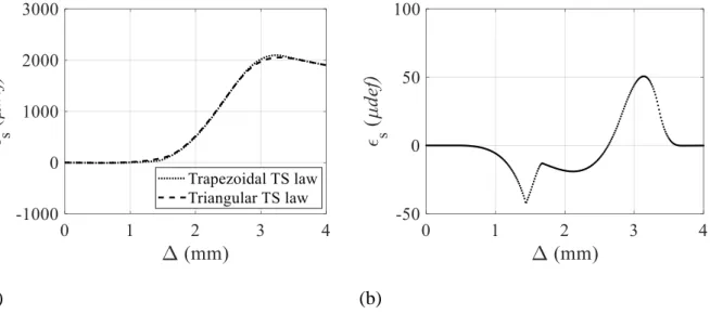
4.3 TS law evaluation from backface strain monitoring technique – BSM
Resistive gauges can be placed on the adherend’s upper face. The measurement of the slabs deformation gives insight on the stress state of the adhesive bond directly underneath the gauges. They measure the local longitudinal strain, 𝜀𝑠, which is proportional to the local
bending moment M: 𝜀𝑠 = 𝑀 𝐸𝑠𝐼𝑛 𝑡 2 (eq 35)
It also depends on the adherends’ Young modulus E, their quadratic moment I and their thickness t. The gauge evolution can also be used for a direct evaluation of cohesive stresses evolution along the bondline by using the relationship:
𝜎 = −2 𝐸𝐼 𝑤𝑡
𝜕2𝜀 𝑠
𝜕𝑥2 (eq 36)
The gauges response is an indicator of the stress state of the adhesive directly underneath. It is worth noticing that the adherend deformation is maximal when the crack tip is close to the
gauge. Figure 6.a illustrates the gauge response for a bilinear softening and a trapezoidal TS law. Their differences are presented in Figure 6.b. It appears that the variation between the two law shapes is quite small. Their maximal differences appear when the adherend begins to deform and when the crack tip is close to the gauge.
(a) (b)
Figure 6: (a) Gauges deformation function of the opening at loading point for triangular and Trapezoidal CZM; (b) Residual between the triangular and Trapezoidal CZM
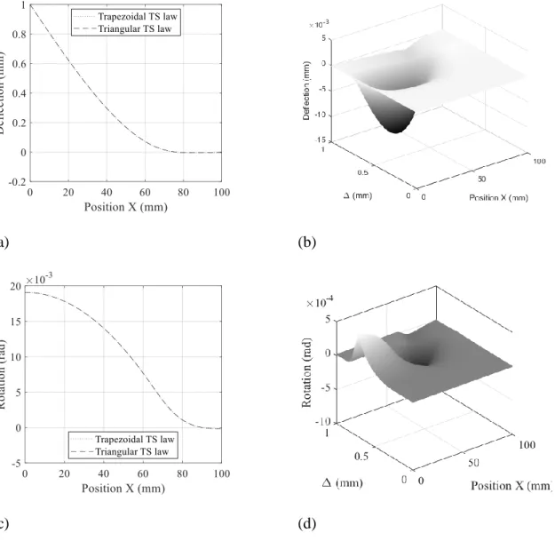
4.4 TS law evaluation from DIC monitoring technique in deflection and rotation
During a DCB test digital image correlation (DIC) can be used to determine the deflection and rotation of the adherends along the bonded area. Experimentally, this requires the use of a speckle pattern and one or a couple of cameras. Numerically the adherends deflection and rotation are directly computed along the specimen. The latter has a different behaviour if the adhesive is in the elastic, the softening or the propagation phase of the CZM. In Figure 7, the deflection and rotation along the adherends are represented for an opening at loading point of 1mm. Their differences are then computed for the whole test, that is to say from Δ=0mm to Δ=1mm with 201 steps in-between. Here, it appears that the deflection of the adherend is not sensitive to the law shape as the differences between both curves is at most 10μm (Figure 7.a
and b). A similar result is found in the rotation case as it is illustrated in Figure 7.c and d, where the maximal deviation is approximately 5.10−4 𝑟𝑎𝑑.
(a) (b)
(c) (d)
Figure 7: Digital image correlation results along the overlap during a DCB test (a) Impact of the TS law on the deflection response for an opening at loading point of 1mm; (b) Residual between the triangular and Trapezoidal CZM for an entire test; (c) Impact of the TS law on
the rotation response for an opening at loading point of 1mm; (d) Residual between the triangular and Trapezoidal CZM for an entire test.
5 Robustness analysis
5.1 Model’s parameters
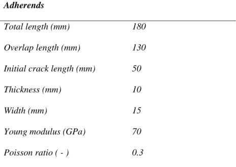
The analytical model, presented earlier, is used to simulate a DCB specimen. Its geometrical and material characteristics are summarized in Table 2.
Table 2: DCB specimen geometric and material characteristics
Adherends
Total length (mm) 180
Overlap length (mm) 130
Initial crack length (mm) 50
Thickness (mm) 10
Width (mm) 15
Young modulus (GPa) 70
Poisson ratio ( - ) 0.3
The adhesive has a chosen thickness of 247µm and is implemented using a trapezoidal cohesive zone model. The parameters of interests are arbitrarily chosen: the initial modulus the maximum stress and the displacement jump at propagation: a = [Ea, σmax, vp]. Table 3
includes the chosen nominal parameters and the associated critical energy release rate in mode I and surface area under the linear part, respectively Gc and Y0.
Table 3: CZM properties Adhesive TS law 𝐸𝑎 (MPa) 146 𝜎𝑚𝑎𝑥(MPa) 14 𝑣𝑝(µm) 56.56 𝑌0 (N/mm) 0.67
𝐺𝑐 (N/mm) 1.42
Experimental data are generated from the known trapezoidal nominal response on which a normal noise is introduced. Every experimental curve comports 201 points taken for the same opening at loading point. This numerical noise represents the experimental data variations that are caused by errors in the measurement chain (i.e. Load captors, gauges, DIC...). For each mechanical response, a custom noise has been applied. It is generated as a normal distribution, the average of which is equal to zero and its standard deviation is approximately 0.5% of the maximal mechanical response. For each method, the tailored noise distributions are summed up in Table 4.
Table 4: Synthetic Noise normal distribution for each mechanical response
Method Units 𝝈𝒏𝒐𝒊𝒔𝒆
P(Δ) N 3.3
J(,) kJ/m² 7
Gauges μdef 10
DIC - deflection mm 0.005
DIC – rotation rad 9.10−5
The minimization of a bilinear softening TS law onto the synthetic data generated from the trapezoidal law was carried out for each mechanical response that can be obtained on a DCB test (i.e. P(Δ) , J(,), Gauges, DIC). However, for clarity purpose, the process will only be detailed for the force-displacement curve and the DIC.
5.2 Methodology application to the Force-displacement curve
The analytical model described in paragraph 2 is used to generate a nominal P(Δ) curves for the trapezoidal TS law. Synthetic experimental data which consists in the addition of a
Gaussian noise as then generated and are illustrated in Figure 8.a. These data are then used for a minimization procedure using the χ² optimisation. Its general principle and equations are exposed in Appendix II. The objective is to apply the minimization to the parameters of the bilinear softening TS law. Figure 8.b displays the P(Δ) curve obtained from the optimized parameters. The residual between the synthetic experimental data and the optimisation results can then be calculated. It can also be extended to a comparison of the nominal trapezoidal law as it is showed in Figure 8.c.
(a) (b)
(c) (d)
Figure 8: Load-displacement curves: (a) Synthetic measurements data for an trapezoidal TS law; (b) Synthetic measurements data with its optimisation result for a bilinear softening TS
law; (c) Residuals between the minimized curve, the synthetic measurements and the nominal trapezoidal TS law; (d) Residual of the nominal and minimized triangular law.
From this analysis, it appears that the minimization enables the determination of a parameter-triplet that has a correlation to the synthetic data as good as the nominal trapezoidal TS law.
Figure 8 also illustrates the difference between the nominal triangular law (that has the same
Ea and σmaxthan the trapezoidal law). The variation of these two parameters enables a
diminution of the highest peak at the cost of deviation in the elastic part.
The computation of the correlation coefficient, R², between the experimental data and either the nominal trapezoidal law or the optimized bilinear softening law, shows that they are equal.
Table 5: Correlation coefficient obtained for the synthetic experimental data Nominal Trapezoidal Optimized bilinear softening
R² 1 0.9999
However, this correlation quality is obtained at the cost of the TS law parameters. As illustrated in Table 6, the parameters obtained by the minimisation are deviating significantly from the nominal values especially for Ea and σmax. Even so, the critical energy release rate
computed is still close to the nominal one, which is coherent as the DCB test was originally made for its estimation.
Table 6: Minimized bilinear softening TS law parameters compared to the nominal trapezoidal parameters.
𝑬𝒂 (MPa) 𝝈𝒎𝒂𝒙(MPa) 𝒗𝒑(µm) 𝑮𝒄 (N/mm)
Nominal trapezoidal 146 14 56.56 1.4178
Minimized bilinear softening 114 19.4 72.98 1.4181
Therefore, the use of inverse analysis on the P(Δ) data does not appear to be robust to the TS law shape. Indeed, for this mechanical response, it is possible to identify a bilinear softening parameters triplet that has a correlation coefficient as good as the nominal trapezoidal one used to generate the data. This leads to an erroneous estimation of the parameters. Thus, this mechanical response does not enable the discrimination of the law shape and must only be used when the TS law shape is known beforehand.
5.3 Comparisons
The methodology presented above was carried out for each mechanical response. The individual results and figures are given in Appendix III. It appears that the results of each mechanical response are similar to P(Δ). Indeed, the minimized curves obtained for a bilinear softening have a correlation coefficient equal to the one obtained for the nominal trapezoidal which was used to generate the experimental data as illustrated in Table 7.
Table 7: R² evaluation between the experimental data and either the nominal trapezoidal or the minimized bilinear softening curve for each mechanical response
Nominal trapezoidal Optimized bilinear softening
P(Δ) 1 0.9999
J(,) 1 0.9999
Gauges 0.9999 0.9999
DIC - deflection 0.9999 0.9999
DIC – rotation 0.9999 0.9999
Moreover, no mechanical response enables a good estimation of the TS law parameters as it can be seen in Table 8. However, the critical energy release rate is well predicted which corroborates the good correlation between the experimental data and the optimised ones.
𝑬𝒂 (MPa) 𝝈𝒎𝒂𝒙(MPa) 𝒗𝒑(µm) 𝑮𝒄 (N/mm) Nominal trapezoidal 146 14 56.56 1.4178 P(Δ) 114 19.4 72.98 1.4181 J(,) 98 20.46 69.33 1.4185 Gauges 137 18.5 76.84 1.4211 DIC - deflection 120 19.21 73.87 1.4189 DIC – rotation 122 19.23 73.91 1.4214 6 Conclusion
An experimental campaign has been carried out based on an analytical model. It was used to determine whether or not the different mechanical fields measurable on a DCB test specimen are robust to the adhesive traction-separation law shape. To do so, a bilinear softening CZM was optimised on experimental data generated from a trapezoidal using the χ² minimisation. Their correlation coefficients as well as the parameters of the nominal and optimized TS law where then compared.
To conclude, it appears that the noisy experimental data cannot be uniquely described by one TS law shape. Indeed, the inverse analysis on experimental data generated from a trapezoidal TS law gives a good correlation when identified with a bilinear softening law shape. This means that none of the mechanical response investigated here enables discrimination to the law shape. Moreover, this inverse identification enables the determination of a TS law parameter-triplet that are not equal to the nominal ones. That is to say that when the inverse identification is made with one of the techniques described in this paper, it is possible to identify cohesive properties. But if the TS law shape has been chosen arbitrarily rather than being measured, this means that these properties are likely to be incorrect. The only reliable parameter which can be used is the critical energy release rate.
As a consequence the inverse identification method should be used with precautions concerning the mechanical phenomena arising within the adhesive bond. Indeed, it enables the determination of a law which will give correct macroscopic results and that could be sufficient when dimensioning parts. But, these results cannot be used as information on the inherent mechanical properties of the adhesive.
7 Acknowledgment
As part of the collaborative project S3PAC (FUI 21), this work was co-funded by BPI France, the Occitanie region and the Nouvelle Aquitaine region.
References
[1] Barenblatt, G. I. The mathematical theory of equilibrium cracks in brittle fracture, Adv.
App. Mech. 1962, 7,. 55-129. DOI: 10.1016/S0065-2156(08)70121-2.
[2] Dugdale, D. S. Yielding of steel sheets containing slits, J Mech. Phys. Solids. 1960, 8, 100-104. DOI: 10.1016/0022-5096(60)90013-2.
[3] Elices M. G. G. V.; Guinea, G. V. ; Gomez J.; Planas, J. The cohesive zone model: advantages, limitations and challenges, Eng. Fract. Mech. 2002,. 69, 137-163. DOI: 10.1016/s0013-7944(01)00083-2
[4] Sørensen, B. F. Cohesive laws for assessment of materials failure: Theory, experimental methods and application, Sørensen, Bent F. Cohesive laws for assessment of materials failure: Theory, experimental methods and application. Risø DTU-National Laboratory for Sustainable Energy, 2010.
[5] Turon, A.; Camanho, P. P.; Costa, J.; Renart, J. Accurate simulation of delamination growth under mixed-mode loading using cohesive elements: definition of interlaminar strengths and elastic stiffness, Compos. Struct. 2010, 92, 1857-1864. DOI: 10.1016/j.compstruct.2010.01.012.
[6] Khoramishad, H.; Hamzenejad, M.; Ashofteh, R. S. Characterizing cohesive zone model using a mixed-mode direct method, Eng. Fract. Mech. 2016, 153, 175-189. DOI: 10.1016/j.engfracmech.2015.10.045.
[7] de Moura, M. F. S. F.; Gonçalves, J. P. M.; Fernandez, M. V. Fatigue/fracture characterization of composite bonded joints under mode I, mode II and mixed-mode I+ II, Compos. Struct. 2016, 139, 62-67. DOI: 10.1016/j.compstruct.2015.11.073
environmental degradation of adhesively bonded aluminium and composite joints using a CZM approach, Int. J. Adhes. Adhes. 2007, 27, 505-518. DOI: 10.1016/j.ijadhadh.2006.09.015.
[9] Högberg, J. L.; Sørensen, B. F.; Stigh, U. Constitutive behaviour of mixed mode loaded adhesive layer, Int. J. Solids. Struct. 2007, 44, 8335-8354. DOI: 10.1016/j.ijsolstr.2007.06.014.
[10] Scheider, I.; Brocks, W. The effect of the traction separation law on the results of cohesive zone crack propagation analyses, Key. Eng. Mater. 2003, 251, 313-318. DOI: 10.4028/www.scientific.net/kem.251-252.313.
[11] Gheibi, M.; Shojaeefard, M. & Saeidi Googarchin, H. Direct determination of a new mode-dependent cohesive zone model to simulate metal-to-metal adhesive joints, J.
Adhesion. 2019, 95, 943-970. DOI: 10.1080/00218464.2018.1455145.
DOI: 10.1016/j.compstruct.2017.09.012.
[12] Xu, Y.; Guo, Y.; Liang, L.; Liu, Y.; Wang, X. A unified cohesive zone model for simulating adhesive failure of ,Composite Structures and its parameter identification,
Compos. Struct. 2017, 182, 555-565. DOI: 10.1016/j.compstruct.2017.09.012.
[13] Škec, L. Identification of parameters of a bi-linear cohesive-zone model using analytical solutions for mode-I delamination, Eng. Fract. Mech. 2019, 214, 558-577. DOI: 10.1016/j.engfracmech.2019.04.019.
[14] Kafkalidis, M. S.; Thouless, M. D.; Yang, Q. D.; Ward, S. M. Deformation and fracture of adhesive layers constrained by plastically-deforming adherends, J. Adhes. Sci.
Technol. 2000, 14, 1593-1607. DOI: 10.1016/j.engfracmech.2019.04.019.
[15] Shen, B.; Paulino, G. H. Direct extraction of cohesive fracture properties from digital image correlation: a hybrid inverse technique, Exp. Mech. 2011, 51, 143-163. DOI:
10.1007/s11340-010-9342-6.
[16] Tsouvalis, N. G.; Anyfantis, K. N. Numerical prediction of the response of metal-to-metal adhesive joints with ductile adhesives, App. Mech. Mater. 2010, 24, 189-194. DOI: 10.4028/www.scientific.net/AMM.24-25.189.
[17] Song, S. H.; Paulino, G. H.; Buttlar, W. G. Influence of the cohesive zone model shape parameter on asphalt concrete fracture behavior, AIP Conference Proceedings 2008, 1, 730-735. DOI: 10.1063/1.2896872.
[18] Zhang, J.; Wang J.; Yuan, Z.; Jia, H. Effect of the cohesive law shape on the modelling of adhesive joints bonded with brittle and ductile adhesives, Int. J. Adhes. Adhes. 2018, 85, 37-43. DOI: 10.1016/j.ijadhadh.2018.05.017.
[19] Volokh, K. Y. Comparison between cohesive zone models, Commun. Numer. Meth. En. 2004, 20, 845-856. DOI: 10.1002/cnm.717.
[20] Alfano, G. On the influence of the shape of the interface law on the application of cohesive-zone models, Compos. Sci. Techno.l 2006, 66, 723-730. DOI: 10.1016/j.compscitech.2004.12.024.
[21] Campilho, R. D.; Banea, M. D.; Neto, J. &. d. S. L. F. Modelling adhesive joints with cohesive zone models: effect of the cohesive law shape of the adhesive layer, Int. J.
Adhes. Adhes. 2013, 44, 48-56. DOI: 10.1016/j.ijadhadh.2013.02.006.
[22] Fernández-Cañadas, L. M.; Iváñez, I.; Sanchez-Saez, S. Influence of the cohesive law shape on the composite adhesively-bonded patch repair behaviour, Compos.Part B-Eng. 2016, 91, 414-421. DOI: 10.1016/j.compositesb.2016.01.056.
[23] de Sousa, C.; Campilho, R.; Marques, E.; Costa, M. & Da Silva, L. Overview of different strength prediction techniques for single-lap bonded joints, P. I. Mech. Eng. L-J Mat. 2017, 231, 210-223. DOI: 10.1177/1464420716675746.
[24] Gustafson, P. A.; Waas, A. M. The influence of adhesive constitutive parameters in cohesive zone finite element models of adhesively bonded joints, Int. J. Solids. Struct. 2009, 46, 2201-2215. DOI: 10.1016/j.ijsolstr.2008.11.016.
[25] Chandra, N.; Li, H.; Shet, C.; Ghonem, H. Some issues in the application of cohesive zone models for metal--ceramic interfaces, Int. J. Solids. Struct. 2002, 39, 2827-2855. DOI: 10.1016/s0020-7683(02)00149-x.
[26] Sørensen, B. F.; Jacobsen, T. K.Determination of cohesive laws by the J integral approach, Eng. Fract. Mech. 2003, 70, 1841-1858. DOI: 10.1016/s0013-7944(03)00127-9.
[27] Rice, J. R. A path independent integral and the approximate analysis of strain concentration by notches and cracks, J. Appl. Mech. 1968, 35, 379-386. DOI: 10.1016/s0013-7944(03)00127-9.
[28] Andersson, T.; Biel, A. On the effective constitutive properties of a thin adhesive layer loaded in peel, Int. J. Fract. 2006, 141, 227-246. DOI: 10.1007/s10704-006-0075-6. [29] Andersson, T.; Stigh, U. The stress--elongation relation for an adhesive layer loaded in
peel using equilibrium of energetic forces, Int. J. Solids. Struct. 2004, 41, 413-434. DOI: 10.1016/j.ijsolstr.2003.09.039.
[30] De Moura, M. F. S. F.; Gonçalves, J. P. M.; Magalhães, A. G. A straightforward method to obtain the cohesive laws of bonded joints under mode I loading, Int. J. Adhes. Adhes. 2012, 39, 54-59. DOI: 10.1016/j.ijadhadh.2012.07.008.
[31] Lélias, G.; Paroissien, E.; Lachaud, F.; Morlier, J. Experimental characterization of cohesive zone models for thin adhesive layers loaded in mode I, mode II, and mixed-mode I/II by the use of a direct method, Int. J. Solids. Struct. 2019, 158, 90-115. DOI: 10.1016/j.ijsolstr.2018.09.005.
[32] Carlberger, T.; Stigh, U. Influence of layer thickness on cohesive properties of an epoxy-based adhesive—an experimental study, J. Adhesion. 2010, 86, 816-835. DOI: 10.1016/j.ijsolstr.2018.09.005.
[33] Mostovoy, S.; Ripling, E. J. Fracture toughness of an epoxy system, J. Appl. Polym. Sci. 1966, 10, 1351-1371. DOI: 10.1002/app.1966.070100913.
[34] Gunderson, J. D.; Brueck, J. F.; Paris, A. J. Alternative test method for interlaminar fracture toughness of composites, Int. J. Fract. 2007, 143, 273-276. DOI: 10.1007/s10704-007-9063-8.
[35] Paroissien, E.; Silva, D. a. L. F. M.; Lachaud, F. Simplified stress analysis of functionally graded single-lap joints subjected to combined thermal and mechanical loads, Compos. Struct. 2018, 203, 85-100. DOI: 10.1016/j.ijadhadh.2017.05.003.
Appendix I. Analytic model validation with the Macro-element model 1 Bilinear softening CZM
In order to validate the analytic solution, a comparison has been made with the macro-element (ME) model developed by Paroissien et al [35]. It is based on simplified hypotheses to model the joint behaviour and uses the minimization of the potential energy for solving. Both the adhesive layer and the adherends are gathered in 4-node elements. The upper and lower adherends’ nodes at the extremity of the specimen are blocked in the normal and tangential direction as well as in rotation. The model dimensions are the same than the analytic ones. Adherends are modelled with a linear elastic behaviour with aluminium mechanical properties (i.e. E=70 GPa, υ=0.3). The adhesive behaviour has been implemented with a bilinear cohesive zone model. The traction separation law is defined by the initial adhesive modulus (Yt=146 MPa), the tensile stress at crack propagation (σmax=14 MPa) and the fracture energy
(Gc=1.4178 N/mm). The parameters used are listed in table 1.
A mesh convergence study has been realized in order to validate the model. The elements size is determined as a ratio of the process zone size 𝐿𝑐. Its size has been estimated using the Irwin
equation:
𝐿𝑐 = 2 𝜋
𝑌𝑡𝐺𝐼𝑐
𝜎𝑚𝑎𝑥2 (eq 37)
Table 9 : FE model mesh size
Lc ratio Element size (mm)
𝐿𝑐 0.67
𝐿𝑐
2 0.34
𝐿𝑐
𝐿𝑐
8 0.08
For each mechanical response the maximum load, the opening at maximum load and critical energy release rate are compared between the analytical model and the ME. It appears that from a density of 4 elements in 𝐿𝑐, the macroelements results converge to the analytical one
for both the triangular and the trapezoidal law shape.
(a) (b)
(c)
Figure 9: ME convergence study for a bilinear softening TS law: (a) Maximum load function of the ME number; (b) Maximum opening at loading point function of the ME number; (c) Critical energy release rate function of the ME number.
(a) (b)
(c)
Figure 10: ME convergence study for a perfectly trapezoidal TS law: (a) Maximum load function of the ME number; (b) Maximum opening at loading point function of the ME number; (c) Critical energy release rate function of the ME number
Appendix II. χ2 minimisation
Obtaining model parameters from a set of experimental data can be achieved with different techniques. The most common technique consists in minimizing an error function which may exhibit significantly non-linear behaviour. In the following, least square minimization is realised considering the Chi square, 𝜒2, function defined with relation:
𝜒2(𝑎) = ∑ [𝑌(𝑡𝑖) − 𝑌̂(𝑎, 𝑡𝑖) 𝜎𝑌(𝑡𝑖) ] 2 𝑛𝑑 𝑖=1 (eq 38)
In (eq 38) Y(ti), i={1,…,N} represent the N measured data used to identify the 𝑎𝑘 k={1,…,p}
parameters. 𝑌̂ are the corresponding theoretical data obtained with the model. In (eq 38), the term in the sum are weighted by the measurement error on the experimental data. This function is minimized using steepest gradient technique such as Levenberg-Marquart algorithm until the minimum 𝜒2value is found and the corresponding optimum set of
parameters is determined. The quality of the optimization process can then be evaluated using the R²-value (eq 39) and (eq 40).
R² =∑ (𝑌(𝑡𝑖) − 𝑌̂(𝑝, 𝑡𝑖)) 2 nd i=1 ∑ni=1d (𝑌(𝑡𝑖) − Y̅(t𝑖))2 (eq 39) with Y ̅(t𝑖) = 1 𝑛𝑑∑ 𝑌(𝑡𝑖) 𝑛𝑑 𝑖=1 (eq 40)
The fit quality is assessed when the R2 value is as close to one as possible.
From a technical standpoint, the curve fitting is performed using the lsqnonlin function implemented in Matlab using the Levenberg-Marquardt algorithm. In order to obtain a more accurate optimization, the gradients were estimated with central finite differences.
Appendix III. Minimization results
The same methodology than in paragraph 5.2 is applied for the other mechanical response.
1. J(,) minimization results
Synthetic experimental data are generated from the nominal trapezoidal law with a Gaussian noise of 7kg.m² (Figure 11a). A triangular TS law is fitted on these data (Figure 11b).and the residual between the synthetic experimental data and the optimisation results is computed
(Figure 11c).
(a) (b)
(c)
Figure 11: Integral J curves: (a) Synthetic measurements data for a trapezoidal TS law; (b) Synthetic measurements data with its optimisation result for a bilinear softening TS law; (c)
Residuals between the minimized curve, the synthetic measurements and the nominal trapezoidal TS law.
2. Gauges minimization results
Synthetic experimental data are generated from the nominal trapezoidal law with a Gaussian noise of 10μm (Figure 12a). A triangular TS law is fitted on these data (Figure 12b).and the residual between the synthetic experimental data and the optimisation results is computed
(Figure 12c).
(a) (b)
(c)
Figure 12: Gauges measurements: (a) Synthetic measurements data for a trapezoidal TS law; (b) Synthetic measurements data with its optimisation result for a bilinear softening TS law;
(c) Residuals between the minimized curve, the synthetic measurements and the nominal trapezoidal TS law.
3. DIC – deflection minimization results
Synthetic experimental data are generated from the nominal trapezoidal law with a Gaussian noise of 5μm (Figure 13a). A triangular TS law is fitted on these data (Figure 13b).and the residual surface between the synthetic experimental data and the optimisation results is computed (Figure 13c). The residual surface between the nominal trapezoidal data and the minimized triangular date is displayed in Figure 13d.
(a) (b)
(c) (d)
Figure 13: DIC – deflection curves: (a) Synthetic measurements data for an trapezoidal TS law; (b) Synthetic measurements data with its optimisation result for a bilinear softening TS
law at Δ = 2 mm; (c) Residuals between the minimized curve, the synthetic measurements and the nominal trapezoidal TS law; (d) Residuals between the minimized curve and the nominal trapezoidal TS law.
4. DIC – rotation minimization results
Synthetic experimental data are generated from the nominal trapezoidal law with a Gaussian noise of 5μm (Figure 14a). A triangular TS law is fitted on these data (Figure 14b).and the residual surface between the synthetic experimental data and the optimisation results is computed (Figure 14c). The residual surface between the nominal trapezoidal data and the minimized triangular date is displayed in Figure 14d.
(a) (b)
Figure 14: DIC – rotation curves: (a) Synthetic measurements data for an trapezoidal TS law; (b) Synthetic measurements data with its optimisation result for a bilinear softening TS law at Δ = 2 mm; (c) Residuals between the minimized curve, the synthetic measurements and the nominal trapezoidal TS law; (d) Residuals between the minimized curve and the nominal trapezoidal law.