Painting recognition from wearable cameras

HAL Id: hal-01062126

https://hal.inria.fr/hal-01062126

HAL is a multi-disciplinary open access

archive for the deposit and dissemination of sci-entific research documents, whether they are pub-lished or not. The documents may come from teaching and research institutions in France or abroad, or from public or private research centers.

L’archive ouverte pluridisciplinaire HAL, est destinée au dépôt et à la diffusion de documents scientifiques de niveau recherche, publiés ou non, émanant des établissements d’enseignement et de recherche français ou étrangers, des laboratoires publics ou privés.

Painting recognition from wearable cameras

Théophile Dalens, Josef Sivic, Ivan Laptev, Marine Campedel

To cite this version:

Théophile Dalens, Josef Sivic, Ivan Laptev, Marine Campedel. Painting recognition from wearable cameras. [Contract] 2014, pp.13. �hal-01062126�

Painting recognition from wearable cameras

Project Report

Théophile Dalens

, Josef Sivic

, Ivan Laptev

, and Marine Campedel

1_{Inria, WILLOW project, Département d’Informatique de l’École normale supérieure,} ENS/INRIA/CNRS UMR 8548, Paris, France

2_{Télécom ParisTech}

Abstract

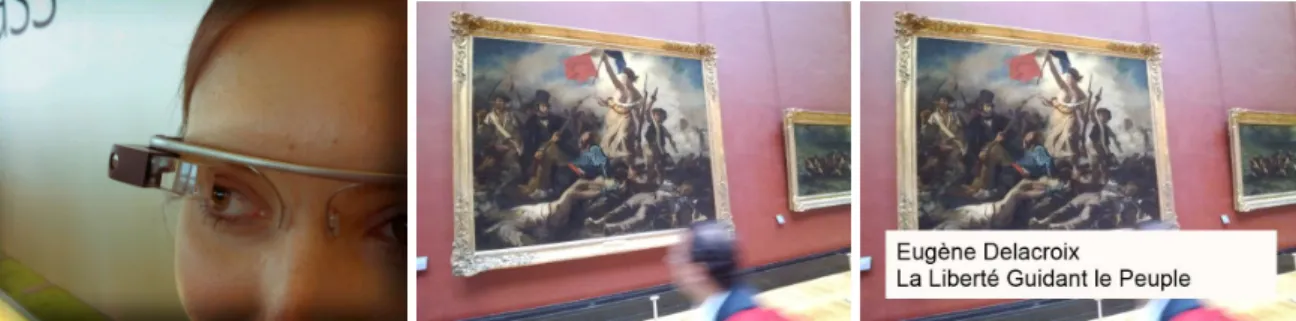
Are smart glasses the new high-tech device that will guide you through a mu-seum? In this report, we describe a system that runs "on device" on Google Glass and retrieves the painting you’re looking at among a set of paintings in a database. We perform an experimental comparison of the accuracy and speed of different feature detectors and descriptors on a realistic dataset of paintings from Musée du Louvre. Based on this analysis we design an algorithm for fast and accurate image matching using bags of binary features. We develop an application that runs di-rectly on Google Glass without sending images to external servers for processing and recognizes a query painting in a database of 100 paintings in one second. The code is available online at [1].

Figure 1: Our application. A Google Glass user (left1) uses our application in a mu-seum to identify a painting (middle). Our application identifies the painting from the database of the museum and displays information such as the name of the painter and the title of the painting (right).

1

Introduction

1.1

Objective

Google Glass is a newly released wearable computer, providing to its user a camera and a display screen, both directly at the level of its eye. Computer vision has many

applications that would benefit the device and its user, including object detection, cat-egorization and retrieval. For example, the device could help its user to identify and describe what he is currently seeing. However, wearable devices have limited process-ing power and available rapid access memory. Therefore, any computer vision-related application must be time and space efficient.

In this work, we aim to develop a method for object retrieval that works in real-time on Google Glass. Our task is to make a painting recognition algorithm, that can match a painting acquired by the device in a museum and match it with the corresponding painting in the database of the museum. The whole application should work in real-time and display information about the painting, like the name of the painter. For this, we detail the general framework of such an algorithm (section 2), consisting of keypoint extraction and descriptors computation, followed if needed by grouping the descriptors into a single image descriptor, and/or geometric verification. In section 3, we compare different approaches for this task, in terms of efficiency and time perfor-mance. Then, in section 4, we detail our implementation and give qualitative results.

1.2

Related work

Using the Google Glass for computer vision has been studied in [2], in which Altwai-jry et al. design a location recognition on Google Glass. In this work, they have a database of images of different buildings and scenes of a city and aim to identify what the user is looking at. They compare different approaches for image description and matching, including the bag of words approach (as described in [17]) with SIFT and SURF descriptors, which performed successfully. However, their approach is different than the one we try to develop in this work, for two reasons. First, they integrate GPS information, which we don’t - our system is designed to work in a very restricted area such as a museum aisle. Secondly, data from the Google Glass is sent to a server for computation. While an online server may have more computational power than the Google Glass, this prevents the system from working without connection to the server and complicates the deployment of the system. Our system is designed to be easy to deploy and work offline, and must face the computational limitations of the wearable device.

2

Overview of the retrieval system

Our system is composed of two distinct parts. First, in the offline part, we compute image descriptors of all the images in our database. This part is done on a computer, and the results are then stored on the Glass. The on device part is the wearable device application. When the application starts, descriptors are loaded into the memory of the device. At the user’s command, the camera on the device captures the query image, and computes the descriptors with the same algorithm as the one used for the offline part. Then, descriptors of the query image are matched to the ones in the database. A match between a descriptor of the query image and a descriptor of the database image is con-sidered good if there is no other descriptor in the database image that matches nearly as well as the first one. The images in the database are then ranked decreasingly ac-cording to the number of good matches they have with the query image. Alternatively, descriptors are matched to visual words to compute a single image descriptor for each image, and we just compare the image descriptors. At last, a geometric verification can

Figure 2: Detected keypoints on a painting with various keypoint detectors, all tuned to detect approximately 500 keypoints: SIFT (top left), SURF (top right), ORB (botttom left) and BRISK (bottom right).

be performed.

2.1

Keypoint detection and descriptors

A capture of a painting by the visitor of the museum, and the painting itself, are differ-ent at various aspects. A geometric transformation is applied (translation and homo-thetic transformation, with also small rotation and perspective transformation), light-ning conditions change and partial occlusions can occur. Hence, it is necessary for our task that image description is as robust as possible to those changes. We consider several possibilities. While SIFT is widely used and is still considered as one of the most robust descriptors, its speed is a concern for real-time applications, leading to the development of descriptors that try to match their performance while being more efficient to compute and to compare. Figure 2 illustrates the various keypoints that can be detected in a painting.

2.1.1 SIFT

Scale Invariant Feauture Transform ([11]) is a classic algorithm to detect keypoints and compute associated descriptors. First, the input image is resampled and smoothed at different scales to create a pyramid of images. Then, keypoints are selected as extrema of differences of Gaussian. Descriptors are then a 128-bin histogram of the differences of Gaussian at different spaces and orientation.

2.1.2 SURF

Speeded-Up Robust Features ([4]), designed as a faster alternative to SIFT, computes an approximation of the Hessian matrix in each pixel of the image at different scales.

Keypoints are selected as the maxima of the Hessian matrix. Descriptors, along with an orientation assignment, are computed as the sums of the responses of patches to wavelets, which result in 64D vectors.

2.1.3 ORB

ORB ([16]) is short for Oriented FAST and Rotated BRIEF. The keypoint detector uses FAST ([15]), a corner detector, combined with a Harris corner detector ([9]), at multiple scales. It also measures a corner orientation. Then, BRIEF ([6]) descriptors are com-puted. A BRIEF descriptors is a bit string of length n, where each bit i equals the result of the test I(xi) < I(yi), I(a) being the intensity of the image I at pixel location a. In

practice, the image is smoothed during this operation: locations xi and yi are chosen

as 5×5 patches in a 31×31 window.

2.1.4 BRISK

Binray Robust Invariant Scalable Keypoints ([10]) is another descriptor that uses FAST keypoints and descriptors that are similar to BRIEF. The main difference is in the sam-pling part that is used to generate the locations xiand yi.

2.2

Matching

To compare SIFT or SURF descriptors, the L2norm is used. Matching binary

descrip-tors is faster, since it uses Hamming distance, which is the number of bits that differ between the two descriptors. To search for the nearest neighbour of a "query" descrip-tor in a set of "database" descripdescrip-tors, we can use brute-force matching, i.e. matching the query descriptor with all the database descriptors and see which gives the highest L2 norm or Hamming distance. However, this method takes time and can be the

bot-tleneck of our system is the set of database descriptors is large.

In [14] and [12], the authors develop forests of randomized k-d trees in order to re-trieve the approximate nearest neighbour of a SIFT descriptor, reducing the complexity of finding the nearest neighbour in a database of size K from O(K) to O(log(K)). For binary descriptors, a classic way to speed up matching is to use locality sensitive hash-ing. Descriptors are hashed into smaller hashes, which are faster to compare. Then, the real descriptor comparison is only done between the ones that have similar hashes.

2.3

Compact image descriptor

Matching the descriptors of the query image to all the descriptors of the database image is not a scalable strategy. Indeed, its complexity is linear with the number of paintings in the database. To solve this issue, the authors of [17] propose a "bag of features", or "bag of words", approach. It consists in building a vocabulary of features, then in representing each image by a histogram. For each image, descriptors are converted into words by taking the approximate nearest neighbour (which is fast with the previ-ous subsection), then the histogram counts the number of occurrences of each word. Histograms are then normalized and re-weighted using tf-idf so that rare words are considered more significant then frequent ones. To match images, we need only match one histogram instead of hundreds of descriptors.

To build the dictionary, the authors of [17] propose to run k-means algorithm to fea-tures extracted from various images, if possible including the images of the database. The k centers are then the k words of the vocabulary. For binary descriptors, the au-thors of [8] replace k-means by k-medians, after "k-means ++" initialization. k-means ++ ([3]) is an algorithm for seeding k-means that select iteratively k initial cluster cen-ters. The first center is chosen according to a uniform distribution. After that, at each step, the distance between each point and its nearest center is computed and squared; the next center is taken randomly according to this distribution. As a result, cluster centers chosen by this algorithm are close to the expected result of the k-means algo-rithm.

2.4

Geometric verification

Once we have potential good matches, we can make use of the spatial repartition of the descriptors in order to retrieve an image that is geometrically consistent. If a query image contains an image of our database, then there exists a geometric transforma-tion, a homography, that matches part of the descriptors of the query image to the database image. To find such a homography, we can use the RANSAC algorithm ([7]), which gives us both the best homography to fit the model and the number of inliers (descriptors that fit the homography). The geometric verification consists in applying this algorithm between the query image and all the best results in our database, then stopping at the first one that gives an important number of inliers. However, each geometric verification takes time to perform.

3

Evaluation of feature extraction and matching

3.1

Database and set up

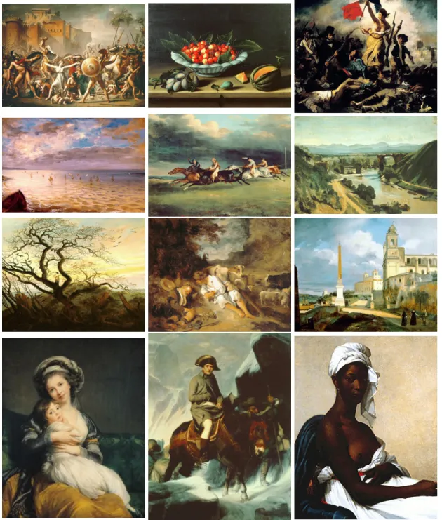
To evaluate our system, we use as a database a set of paintings from Musée du Louvre, collected from a CD-ROM guide of the museum. It includes more than 600 paintings. The resolution of the images is not high (typically 250x350). From these paintings, we have selected a representative set of 100, that include portraits, landscapes and other sceneries. The styles of the paintings are loosely consistent (mainly Italian and French paintings), as to maintain a certain difficulty and to simulate a typical set of paintings in a aisle of the museum. A set of paintings is shown figure 3.

As query images, we use data collected from the Google Glass in the Musée du Lou-vre. We went to the room 77, also called salle Mollien, and to the aisles with the French paintings, from which we casually captured 10 images that include landscapes, por-traits and other sceneries. Each picture has been rescaled using the same factors. They include the typical small occlusions and perspective deformations that can be expected when a visitor looks at paintings. They are shown in figure 4.

For all descriptors, we use the OpenCV [5] implementation.

3.2

Accuracy

To measure the accuracy of the different descriptors, we match the descriptors of com-puted on our input images and the descriptors of the images of our database. Then, we rank the database images decreasingly according to the number of matches. We

Figure 4: Input images used for tests. These paintings are from (top to bottom, then left to right) Corot (3 paintings), David, Lebrun (2 paintings), Delacroix, Géricault, Benoist and Ingres

measure recall at top 1 (number of times that the correct database painting arrives in first position) and recall at top 5 (number of times that the correct painting arrives in at worst at fifth position). The recall at top 5 is interesting because if we complete the matching with geometric verification, having the correct answer in the top 5 will assure that we only need to perform this costly operation on at most 5 images. We have tested the different keypoint detectors and descriptors with various parameters and only display the ones that give the best results (default parameters for SIFT and BRISK, Hessian threshold of 475 for SURF, 1000 keypoints for ORB). We also display the results for ORB with only 500 keypoints, as decreasing the number of keypoints de-creases the computational time for matching. At last, we have found that using SURF keypoints gave better results than the BRISK ones, when using BRISK descriptors. Re-sults are shown table 1.

While all the systems perform similarly for the landscapes, their performance

gener-System Recall at top 1 Recall at top 5

SIFT 90% 90% SURF 70% 90% ORB (500 descriptors) 80% 80% ORB (1000 descriptors) 100% 100% BRISK 60 % 60% SURF+BRISK 80% 100%

Table 1: Performance measurements for the different descriptors. "SURF+BRISK" de-signs a combination of the SURF keypoint detector and the BRISK feature descriptor.

ally decrease for the portraits. ORB performs well every time when it computes enough descriptors; otherwise, the keypoints captured on the images are not dense enough. For the ORB descriptors, we have also evaluated the performance of a bag of features approach. For these tests, we have computed dictionaries of 10,000 and 100,000 words from the extraction of ORB features from each of 600 paintings, including the 100 ones used for testing. The performances are competitive with the previous approach (ta-ble 2).

3.3

Timing

3.3.1 Descriptor extraction

We have measured, on the Glass, the time taken to detect keypoints and compute their descriptors. Comparisons are made on the same input image. Results are displayed in table 3.

As expected, binary features are faster to compute than SURF and SIFT. Time used

System Recall at top 1 Recall at top 5 Bag of ORB (10,000 words) 80% 80% Bag of ORB (100,000 words) 90% 90%

Table 2: Accuracy measurements for the bag of binary features (ORBs). The number of words shown is the size of the vocabulary.

Description method Time for keypoint detection (ms) Time for computation (ms)

SIFT 4180 3,86

SURF 2008 2,47

ORB 109 0,39

BRISK 8106 0,15

Table 3: Time to detect keypoints on a 640x480 picture on the Google Glass, and to compute a single descriptor.

to detect BRISK is unexpectedly high, and most probably comes from a flaw in its OpenCV implementation.

3.3.2 Descriptor matching and hierarchical bag of words

We have also timed binary feature matching. Matching 500 ORB features of a query image with 500 ORB features of a database image takes approximately 400 millisec-onds.

When matching 500 descriptors to a vocabulary of 100,000 words, this matching be-comes the bottleneck of our application. For this reason, we use a hierarchical bag of words, similar the hierarchical k-means described in [13] and [12], but applied here to binary features, and building the tree of features from leaves to roots. From the 100,000 words that have been extracted as a vocabulary, we extract a smaller number of words (typically 500). This new, small vocabulary constitutes another layer in our bag of visual words. Then, we assign each word of the large vocabulary to its k nearest neighbours in the small one (typically k =2). To get a bag of words representation of the descriptors of our image, we match the descriptors of our database with the words of the small vocabulary. Then, we match them with the words of the large vocabulary that are assigned to matched words of the small one.

As a result, the complexity in time of the matching part is in the square root of the size of the vocabulary, instead of being linear. Typically, the 500 descriptors extracted are matched one-to-one with the words of the small vocabulary (500), then with the linked words of the large one (in average 400, up to 2400), which results in less than 1 second of computation. With these parameters, we do not observe drop in accuracy. However, reducing k to 1, which would allow a faster matching, reduces the accuracy significantly.

4

Implementation on Google Glass

The Google Glass is a device running on Android. To implement the on device part on the algorithm, we use Java, C++ (via JNI) and OpenCV. The code described in this report can be found online at [1].

Inspired from the results of section 3, in which we show the efficiency of the ORB descriptors in accuracy and speed, we propose two implementations of our system.

4.1

Implementation using direct feature to feature matching

In the first version, the offline part consists in computing ORB features for all our database. These features are saved into XML files, which are then transferred to the

device at the installation of the application. Then, at the start of the application, these descriptors are loaded. When the user taps the touchpad of the device, an image of what the user is currently seeing is captured. Then, the extraction of the ORB features, matching and ranking of images is performed in C++ and native OpenCV code. The result is handled by the Java part of the application, that has loaded a table with the names of the painters of each painting. Then name of the painter is then displayed.

4.2

Implementation using bag-of-visual-words matching

The second version uses bags of ORB features. In the offline part, we compute a vocab-ulary of 100,000 ORB words. To compute the vocabvocab-ulary, we extract ORB features from the paintings of the database, and perform k-means++ seeding. We then compute the histograms of words for each painting in the database. These histograms are stored into a single sparse matrix. Using a sparse matrix is essential here, to limit both the space and time resources that will be used by the application when loading the matrix and performing comparisons of histograms.

Still in the offline part, we compute a second layer of 500 visual words. These are se-lected via k-means++ from the large vocabulary. Then, each of the words of the large vocabulary is assigned to its 2 nearest neighbours in the small one. These assignments are also saved and stored to the device.

At the start of the Glass application, the histogram, the small and the large vocabu-lary and the assignments are loaded. When the user touches the touchpad, 500 ORB features are extracted from the image captured by the camera, and transformed into words using brute-force matching with the small vocabulary. Then, we match each feature to a word of the large vocabulary whose nearest neighbours include the word of the small vocabulary, using the assignments matrix. The resulting histogram is com-pared to the ones of the database by performing a sparse matrix multiplication. The name of the painter of the image that has the most similar histogram is then retrieved and displayed at the Google Glass screen. The whole process takes approximately 1.0 second.

4.3

Results

While the first version performs successfully most of the time, it is not scalable to many images. With 10 images in the database, it runs in approximately 5 seconds, and the time is expected to be linear with the number of images in the database. Indeed, match-ing features from one image to another takes 0.4 seconds. The second version, on the other hand, performs in 1 second for 100 images. However, it is more slightly more likely to fail and not retrieve the correct painting. A sample of the results is shown figure 5.

5

Acknowledgements

This work was partially funded by the EIT-ICT labs.

Figure 5: Examples of correct and incorrect retrievals of the second method, which is expected to retrieve the correct painting nine times out of ten.

6

Conclusion

In this work, we have compared different descriptors in order to perform object re-trieval, in the context of paintings in a museum. We have successfully implemented on Google Glass a system able to tell a user which painting he is looking at, among the different paintings of a section of a museum. It uses a hierarchical bag of ORB features, which are fast to extract and efficient in matching.

References

[1] GlassPainting code repository.https://github.com/NTheo/GlassPainting, 2014. [2] Hani Altwaijry, Mohammad Moghimi, and Serge Belongie. Recognizing locations with google glass: A case study. In IEEE Winter Conference on Applications of Com-puter Vision (WACV), Steamboat Springs, Colorado, March 2014.

[3] David Arthur and Sergei Vassilvitskii. K-means++: The advantages of careful seeding. In Proceedings of the Eighteenth Annual ACM-SIAM Symposium on Discrete Algorithms, SODA ’07, pages 1027–1035, Philadelphia, PA, USA, 2007. Society for Industrial and Applied Mathematics.

[4] Herbert Bay, Andreas Ess, Tinne Tuytelaars, and Luc Van Gool. Speeded-up ro-bust features (surf). Computer vision and image understanding, 110(3):346–359, 2008. [5] G. Bradski. Dr. Dobb’s Journal of Software Tools.

[6] Michael Calonder, Vincent Lepetit, Christoph Strecha, and Pascal Fua. Brief: Bi-nary robust independent elementary features. In Computer Vision–ECCV 2010, pages 778–792. Springer, 2010.

[7] Martin A Fischler and Robert C Bolles. Random sample consensus: a paradigm for model fitting with applications to image analysis and automated cartography. Communications of the ACM, 24(6):381–395, 1981.

[8] Dorian Galvez-Lopez and Juan D Tardos. Bags of binary words for fast place recognition in image sequences. Robotics, IEEE Transactions on, 28(5):1188–1197, 2012.

[9] Chris Harris and Mike Stephens. A combined corner and edge detector. In Alvey vision conference, volume 15, page 50. Manchester, UK, 1988.

[10] Stefan Leutenegger, Margarita Chli, and Roland Yves Siegwart. Brisk: Binary robust invariant scalable keypoints. In Computer Vision (ICCV), 2011 IEEE Interna-tional Conference on, pages 2548–2555. IEEE, 2011.

[11] David G Lowe. Object recognition from local scale-invariant features. In Computer vision, 1999. The proceedings of the seventh IEEE international conference on, volume 2, pages 1150–1157. Ieee, 1999.

[12] Marius Muja and David G. Lowe. Fast approximate nearest neighbors with au-tomatic algorithm configuration. In International Conference on Computer Vision Theory and Application VISSAPP’09), pages 331–340. INSTICC Press, 2009.

[13] David Nister and Henrik Stewenius. Scalable recognition with a vocabulary tree. In Computer Vision and Pattern Recognition, 2006 IEEE Computer Society Conference on, volume 2, pages 2161–2168. IEEE, 2006.

[14] J. Philbin, O. Chum, M. Isard, J. Sivic, and A. Zisserman. Object retrieval with large vocabularies and fast spatial matching. In IEEE Conference on Computer Vision and Pattern Recognition, 2007.

[15] Edward Rosten, Reid Porter, and Tom Drummond. Faster and better: A machine learning approach to corner detection. Pattern Analysis and Machine Intelligence, IEEE Transactions on, 32(1):105–119, 2010.

[16] Ethan Rublee, Vincent Rabaud, Kurt Konolige, and Gary Bradski. Orb: an effi-cient alternative to sift or surf. In Computer Vision (ICCV), 2011 IEEE International Conference on, pages 2564–2571. IEEE, 2011.

[17] Josef Sivic and Andrew Zisserman. Video google: A text retrieval approach to object matching in videos. In Computer Vision, 2003. Proceedings. Ninth IEEE Inter-national Conference on, pages 1470–1477. IEEE, 2003.