Araar : CIRPÉE, Pavillon J.A. DeSève, Université Laval, Québec, Canada G1K 7P4 Phone : 1-418 656-7507 Fax : 1-418 656-7798
This work was carried out with funding from the Poverty and Economic Policy (PEP) Research Network, which is financed by the International Development Research Centre (IDRC), the Canadian International Development Agency and the Australian Agency for International Development (AusAID). I am also grateful to Jean-Yves Duclos and Sami Bibi for their valuable comments.
Cahier de recherche/Working Paper 08-17
Social Classes, Inequality and Redistributive Policies in Canada
Abdelkrim Araar
Abstract:
The social performance of fiscal redistributive mechanisms in Canada continues to receive a growing interest from politicians and research scientists. The aim of this paper is to assess the evolution of social classes in Canada and to check whether the market and governmental redistribution factors have affected their evolution during the last decade. We focus on the dynamic of inequality, polarization and progressivity of the fiscal system. The results of this study confirm the effectiveness of governmental redistributive mechanism to decrease inequality and polarization significantly and to maintain the middle social class at the detriment of the poorest one. The other evidence concerns the chronic increase in population share and wellbeing of the rich class. Finally, the progressivity of fiscal system has registered a significant increase during the last few years.
Keywords: Social classes, poverty, inequality redistribution
1 Introduction
There is a growing interest on studying the negative aspects of distribution of wealth in developed countries during the last few decades. Indeed, the social economic performance became another objective to be archived, in addition to the macroeconomic performance criteria. During the last few years, Canada was classified among the higher ranked countries according to level of standard of living. In 2007-08, Canada was ranked fourth according to its Human Development Index by the United Nations. In general, the country’s standard of living, health care system, educational attainment, housing, cultural and recreational facilities and level of public safety are all of an exceptional high quality. For the Canadian case, there are two main distributive mechanisms that determine the shape of distribution of the available income to be used by the household after paying taxes and receiving transfers. Firstly, total income of the country is distributed according to endowments of individuals and their interaction with the free markets. Secondly, the governmental interventions, through fiscal system and social programs, adjust the generated distribution of income under the free market forces.
A lot of questions can be raised concerning the evolution of distribution of income during the last few decades. For instance, how do inequalities in market and available household incomes have evolved overtime? What was the impact of the change in market factors and population endowments on average income growth and the distribution? How population size of poor, middle and rich social classes has changed overtime? How do redistributive mechanisms have affected the importance of social classes overtime? Does the evolvement of market environment and fiscal system more favourable for reinsertion of the poor or excluded social group into the economic activity sphere? Is the distribution of income more polarized in last few years? Is the fiscal system more progressive, that is, by supporting the poorer group, in the last few years?
To conduct this study and to shed light on these different preoccupations, we use rich and more updated distributive analysis tools that we present in detail in the following sec-tion. We adopt the net income as the indicator of wellbeing for Canadian households and we use the Survey of Labour and Income Dynamics (SLID), to characterize the evolution of distributive phenomena. The choice of this survey is explained, inter alias, by its national representativeness and its rich information about incomes, taxes and transfers at household level. The survey that we use covers the period 1993 to 2005, but our analysis focuses more on the period after 1996, when SLID survey acquired its full sample size. In addition to us-ing the most updated household survey, we use the most conventional and widely accepted methods to normalize individual wellbeing according to its household composition (number of household member, their age, etc.) and the temporal and spatial variations of prices. These normalizations are required to compare estimated indices across provinces and across time.
The goals of this study are multiple. On the one hand, the different derived results will give us a complete picture of the experienced changes in distribution of wealth during the last decade. On the other hand, the analysis of the link between the different distributive indices will allow us to better understand the nature of the link between them. Finally, conclusions and remarks, drawn in this study, will help policymakers to undertake optimal strategic poli-cies in order to enhance social performance in Canada.
The rest of this paper is organized as follows. In section 2, we present the theoretical framework concerning the distributive analysis tools used in this study. In section 3, we present and discuss the results and we conclude in section 4.
2 Theoretical framework
2.1 Social Classes and Distributive Indices
In general, social class refers to persistent social inequalities. However, how do we de-fine social classes? Historically, there are two main sociological theories. The first one is based on the theory derived from works of Karl Marx, and the other from Max Weber1. The Marxian social class distinctions do not refer to types of occupation or levels of income but on the form of physical and capital endowments that each social group possess. The non-Marxists define social classes through inequalities in income, educational attainment, power and occupational prestige. To define social classes, we adopt Weber’s definition. This choice is justified, inter alias, by the deep change in the organization of economic activity during the last century. Indeed, nowadays, the rank of individuals through the type of endowment they possess may be different from those based on returns or income. For our study, social classes are determined mainly by the indicator of standard of livings, which is income. Hence, each social class is defined by a given income range. For instance, it is widely accepted that the level of income of poor group is limited to the lowest level of income (usually zero) and the poverty line. After dividing the population into useful analytical social classes, one can propose a set of distributive indices to study their importance and their welfare. Formally, if we denote the lower and upper income bounds for a given social class S by LS and US respectively, we can write the following:
i ∈ S if yi ∈ [LS, US], (1) where yi is the income of individual i. From this, one can define two basic indicators at the individual level, which are the gap and the surplus, relatively to its social class. The gap of individual i is defined as follows:
g(S, yi) = (yi− LS), (2) and its surplus is:
s(S, yi) = (US− yi). (3)
Social class distributive indices
As proposed byAraar (1999) and (2005), a set of distributive indices can be derived starting from these two basic indicators. We define the deficit index ISfor the social group S by2:
IS(α) = Z US
LS
g(S, y)αdF (y)dy, (4)
1See for this, Marx (1861-3), Weber (1964), (1978) and Hurst (2007).
2One can remark that the FGT index proposed by Foster, Greer, and Thorbecke (1984), represents a special
where F (y) is the distribution function of incomes. Similarly, the surplus index, for social group S, is defined as:
¯
IS(α) = Z US
LS
s(S, y)αdF (y)dy. (5)
The parameter α is crucial to determine the sense the social class index. When this parameter equals zero, the two social class indices simply equal to the population share of social class. If the parameter α = 1, the deficit index expresses the average gap whereas the surplus index expresses the average surplus of social class. Also, in this case, we can write the following equality:
φS(US− LS) = IS(α = 1) + ¯IS(α = 1). (6) where φS is the population share of group S. When the parameter α > 1 and , the proposed indices are sensitive to the inequality within the social class and the parameter reflects the social aversion to inequality. For instance, if the parameter equals to two, the surplus index of a given social class decreases with an increase in inequality within this class.
The overload index
This index represents the ratio between the deficit index of poor group and the surplus index of non poor group. When the parameter α = 0, this index express the ratio between the number of the poor and that of the non poor. When the parameter α = 1, this index equals the ratio between the average gap of the poor group and average surplus of the non poor group. This ratio also expresses the uniform tax rate that the government can apply on incomes of non poor group to finance the total depth of the poor group. In addition, this indicator gives us an idea about the real capacity of the country or province to deal with poverty phenomenon, through income tax revenues.
2.2 Traditional social classes and distributive analysis
Under their algebraic form, the proposed distributive indices do not restrict the number or the manner of selecting social classes. However, for analytical purposes, one must focus on analyzing the most important social classes. This will be related easily to the social and economic performance. In this study, we focus on the following traditional social classes:
1- The poor social class
The recent years have witnessed an increasingly strong interest in studying poverty. Indeed, during the last few decades, this phenomenon began more pronounced especially in devel-oping countries. Many factors can explain its expansion, like those related to the economic transition or those implied by the economic globalization and the reorganization of economic structures at world level. For developed countries, there is a growing interest to study the social exclusion phenomenon and to propose policies, aimed at facilitating the reinsertion of this group to the economic activity. There is a consensus to define the poor based on its standard of livings. Simply, the individual is judged poor if its income is bellow the poverty line3.
2- The middle social class:
Several economists agree with the importance of a wide middle class. Indeed, a wide middle class may indicate the implication of a large portion of the population to the economic activity, as well as a healthy market mechanism to ensure a more equitable distribution of wealth. Inversely, the small portion of this social class is usually linked to inequality or polarization in distribution of income 4. The natural definition of this social class is by setting its income range between the poverty line and the richness threshold.
3- The rich social class:
The existence of this class is natural in an economy based on free markets. A higher pop-ulation share and welfare level of this group continues to raise mitigated opinions about its impact on economic efficiency and income distribution. Among the virtues of the existence of a rich class is the possibility of accumulation of capital to be injected in vital investments. A bad management of resources of this social class may be disastrous for the economy of the country. By surpassing the method that can adopted to fix the richness threshold, one can say that individuals belonging in this rich group must have an income that exceeds the richness threshold.
2.3 Absolute and relative social class thresholds
Studies on poverty have distinguished two approaches to determine the poverty line. These two approaches are:
The absolute approach:
A measure of absolute poverty quantifies the number of people below a poverty threshold, and this poverty threshold is independent of time and place. For the measure to be absolute, the line must be the same in different countries, cultures, and technological levels. Such an absolute measure should only look at the individual’s power to consume and should be independent of any changes in income distribution. The absolute poverty line measures the cost of basic needs without taking into account the wealth state of the country.
The relative approach:
A measure of relative poverty defines “poverty” as being below some relative poverty threshold. An example is when poverty is defined as households who earn less than 50% of the median income is a measure of relative poverty. Notice that if everyone’s real income in an economy increases, but the income distribution remains the same, relative poverty will also be the same. In general, relative poverty is sensitive to the growth in average income. Analogous to what has been proposed for the poorer social class in poverty studies; one can generalize this and propose these approaches to determine social class thresholds.
2.4 Decomposing variation in social class indices
To show the main factors that have contributed significantly in the variation of social class indices, one can decompose this variation into two main comprehensive components. There are many factors that can influence social class indices, but the most important in our analysis are those related to the economic performance, represented by growth in average income, and those related to redistributive mechanisms5. In developed economies like Canada, two main factors influence the form of the distribution of net income. The first is attributed to individ-ual endowments and market forces. The second is attributed to governmental intervention, through the fiscal system and a set of social programs. Formally, we decompose the observed variation in a given social class index, based on gross income, as follows:
∆IS(α, X) = Cµ1 X→µ2X | {z } Growth + Cπ1 X→πX2 | {z } Redistribution , (7) where µt
X and πtX denote the average income and the distribution of X in time t respectively. To perform this decomposition, we use the Shapley approach, to avoid the arbitrariness in selecting the reference period6. The rule that we adopt to eliminate partially the impact of each factor is as follows:
• To eliminate the impact of growth, we multiply gross incomes by the ratio µ1X
µ2
X.
• To eliminate the redistributive impact, we multiply incomes by the ratioµ2X
µ1
X.
One can report here the following expected impact of growth and redistribution on social class indices. First, growth in average income is expected to decrease the population size of the poor class and increase the richest one. Population size of the middle class may increase, but this depends also on the initial form of distribution of incomes. An increase in inequality may increase substantially the poor and rich classes at the detriment of the middle one. Obviously, the proposed method can be applied to decompose the redistributive effect of fiscal system for a given period as fellows:
ISt(α, N ) − ISt(α, X) = Cµt
X→µtN + CπXt →πtN, (8)
This implies again:
∆IS(α, N ) = ∆IS(α, X) + ∆CµX→µN + ∆CπX→πN. (9)
Staring from this last form of decomposition, if one assume that all collected taxes are re-distributed and if the change in the fiscal system overtime is small, then the change in the structure of social classes is mainly influenced by market forces.
5The assessment of the contribution of growth and changes in inequality to the evolution of poverty
was pioneered by Datt and Ravallion (1992). See also Kakwani (1997) and (1993), Shorrocks (1999), Araar and Awoyemi (2006), and Araar and Duclos (2007b) for this issue.
2.5 Inequality and polarization
Even if the estimation of different social class indices may give us a general picture of social class structure, as well as the form of the distribution of income in Canada, it will be useful to summarize information about the level of inequality or polarization with a unique index to be easily comparable across time or across population groups. In this study, we use the popular Gini index to assess inequality and theFoster and Wolfson (1992) (FW) and
Duclos, Esteban, and Ray (2004) (DER) indices to assess bipolarisation and polarization
re-spectively. Formally, the normalized DER index can be written as follows:
PDER = A Z Z
f (x)1+αf (y)|x − y|dydx, (10) where A = 0.5µα−1 and f (.) is the density function. One can recall that, when the parameter
α = 0, the normalized DER index equals the usual Gini index. The question that can now
be raised is: How do polarization indices differ from those of inequality? While inequality measurements are conceived to assess the expected divergence or disparity between incomes, polarization measurements are also sensitive to the level of identification of groups through income. For a given population group delimited by a small income range, its identification increases with its population share7. Furthermore, it has been argued for the evident link between polarization and some other negative aspects of the distribution. For instance, se-vere poverty, disappearance of middle class or higher level of between-group inequality are certainly related with polarization phenomenon.
Now, we review the adopted bipolarization measurement. Bipolarisation can be viewed as a special case of polarization when one focuses on the level of disparity and identification of the two main groups of the population. For the FW index, the first group is composed from those with income bellow the median and the second with income above this threshold. An interesting representation of this index was proposed byRodrguez (2004):
PW OLF = 2µ m £ IGB m− IGWm ¤ (11) where IGB
m and IGWm are the between and within inequality components, when the Gini index is decomposed by the two population groups, separated by the median of income (m). Hence, the FW index reaches its maximum when the first half of the population has a null income and the second one shares equally the total income. In general, any distributive change, which increases the average income of the rich group will increase bipolarisation measurements. In addition, a decrease in inequality within any of these two groups will increase the bipolarisation (groups will be more identified through income). In summary, this index gives us synthesized information about the level of disparity in average income between the two main groups of population and how these two groups are homogeneous based on their income levels.
2.6 Testing progressivity of fiscal system
Usually in distributive analysis, we assess the progressivity of taxes or transfers. However, with governmental intervention through fiscal system, the household can have, depending on
its characteristics, a simplified negative or positive impact on its gross income. First, we begin by dividing the total impact of fiscal system on household income, which is the difference between net and gross income, into two main components. If the impact at household level is negative, we assume that the latter represents a global tax, noted by T that the household must pay. In contrast, if the impact is negative, this represents a global transfer that the household receive and we denote it by B. One must recall that a tax is progressive if the tax burden of the poor group is relatively lower than that of non poor group. This implies a rise in the share of net income for the poor group. In the literature of progressivity, there are two main distinct concepts of progressivity, which are the local progressivity and the global
progressivity. In the pioneered work of Musgrave and Thin (1948), two main approaches were proposed for the measurement of local progressivity, which are the liability progression and residual progression. Let V (x) denotes the final impact on gross income x, such that
V (x) = B(x) − T (x).
Theorem 1 With the liability progression measurement, a fiscal system with tax T and
trans-fer B is locally progressive if and only if: LP (x) = B(x) x ηB(x) − T (x) x ηT(x) − V (x) x < 0, (12)
where ηT and ηB refer to the elasticities of tax T and transfer B with respect to income x respectively.
Proof. This condition can be easily derived starting from the initial condition of local progressivity of the net benefit V (x), which is: ηV (x) < 1.
One can recall here that with the residual progression measurement, a fiscal system with tax T and transfer B is locally progressive if and only if8:
RP (x) = ηN (x) < 1, (13)
ηN(x) refers to the elasticity of the net income N(x) with respect to income x. To test the global progressivity of a fiscal system, we use two dual approaches. The first is the Tax
Redistribution approach (T R), which is based on the distribution of taxes considering that
of gross income. The second is the Income Redistribution approach (IR), which is based on the distribution of net income considering that of gross income.
Theorem 2 A fiscal system with tax T and transfer B is globally T R progressive if and only
if: T R(p) = µT µX [L(p) − CT(p)] + µB µX [CB(p) − L(p)] > 0 ∀p ∈ [0, 1], (14) where µT and µBare the average tax and average transfer respectively.
Proof. The link between concentration curves and progressivity was already developed
byKakwani (1977). Araar (2002) andDuclos and Araar (2006) -section 12.8-, prove that the
proposed hybrid curve is equal to the change in Lorenz curve with a marginal change in taxes and transfers.
One can check easily that if T R(p) is greater than zero for all the range of percentiles, and in absence of re-ranking, the redistributive effect of this fiscal system is socially efficient and inequality must decrease. Instead of comparing between Lorenz and concentration curves, one can propose to use progressivity indices. The aim of these indices is to capture the whole progressivity with one synthetic index9. In general, these indices are computed as differences between the Gini and concentration indices.
Corollary 3 A fiscal system with tax T and transfer B is progressive if the index of
progres-sivity: µT µX [ICT − IGX] + µB µX [IGX − ICB] > 0 , (15) where IG and IC are the Gini and concentration indices respectively. For the IR approach, one can recall that the fiscal system is IR progressive if:
IR(p) = [CX−T +B(p) − Lx(p)] > 0 ∀p ∈ [0, 1], (16) where Lx(p) and Cx(p) denote the Lorenz and concentration curves respectively at percentile
p. Using Gini and concentration indices, one can recall that the fiscal system is progressive
if:
IGX − ICX−T +B > 0 . (17) To assess the nature of change in global progressivity of fiscal system across time, it is not sufficient to compare the progressivity indices, estimated for each year. Indeed, the ab-sence of the common support of comparison for progressivity across years may mitigate our conclusion. Clearly, the change in the pre-tax income distribution can affect the progressivity measurements with an unchanged fiscal system10. The less equal is the pre-tax income distri-bution, the greater will be the equalizing effects and hence the global index of progressivity of a given progressive tax structure. Hence, progressivity indices cannot be compared with the change in the distribution of gross income from one year to another11. To address this issue, we propose to compare between progressivity indices or curves, when the reference year is predetermined. For instance, to compare the progressivity of a tax system between periods 1 and 2, when the period of reference is the first, one can use the information about gross income, tax and transfers of period 1 and estimate the expected taxes and transfers of period 1, using information of period 2 (explanatory variables of period 2). Practically, one can use the kernel non parametrical approach to estimate these expected taxes and transfers. The same exercise may be done using period 2, as the reference period. Again, in this con-text, the Shapley approach can be used to avoid the arbitrariness in selecting the reference period12.
9See Duclos and Araar (2006), chapters 7 and 8.
10For the measurement of the global progression, Musgrave and Thin (1948) has proposed to use the relative
change in equality implied by the tax. However they note that this change depends on the initial distribution of pre-tax income.
11See Kasten (1994), Thoresen (2002) and Kesselman and Cheung (2004). 12See for instance Araar and Duclos (2003)
3 Application
3.1 The Canadian household income surveys
The SLID surveys
To assess the level of distributive phenomenon, like inequality or polarization, one has to select beforehand the unit of analysis, the indicator of wellbeing and the covered population. Since there is no available information about wellbeing or income for the whole population, we usually use national representative surveys to estimate values of distributive indices and to infer them statistically to the total population. For this study, we adopt the net income as the indicator of wellbeing for Canadian households and we use the SLID cross-section survey to assess the evolution of distributive phenomena. The choice of this survey is explained, inter alias, by its representativeness at national level and its rich information about incomes, taxes and transfers at household level. Introduced in 1993, SLID provides an added information, which is the changes experienced by individuals and families through time. Since 1996, the SLID survey officially replaced the annual Survey of Consumer
Finances (SCF). SLID contains a part of longitudinal data, and where the same people were
interviewed from one year to the next for a period of six years. The survey’s longitudinal dimension allows evaluation of concurrent and often related events. In this paper the SLID survey covers the period 1993 to 2005.
Change in SLID coverage overtime
It is well known that different coverage surveys will produce slightly different estimates. One can recall that the SLID only acquired its full sample size in 1996. As reported by Statistic Canada, for the SLID survey, there has been a noticeable upward or downward shift in a data series between the years 1995 and 199613. One must distinguish between the change in the data which is attributable to the two surveys having different samples and different methods (such as the use of tax data in the case of SLID) and the change in the characteristics of the population. Based on this, the observed break in derived results before and after the 1995/96 period must be less informative and attributed mainly to the change in Data. For this reason, even if we report results for the years before 1996, we concentrate more on describing and interpreting results of the period 1996-2005.
3.2 Unit of analysis and indicator of wellbeing
There is a consensus on the relevance of using the individual as the main unit of dis-tributive analysis and to ensure an accurate estimation of wellbeing for household members. Hence, the primary step is to assess wellbeing of individuals and one has to adjust the total household income by the family size and its composition. The simplest method is to use per capita income, that is, to divide the household income by the household size. Unfortunately, this method underestimates the economic wellbeing for larger households as compared to smaller households. This can be explained mainly by economies of scale, realized within the largest household. In addition, basic needs may differ according to age and gender of
hold members. To take into account these different aspects, the widely accepted method is to use the size of equivalent adult to adjust total income for household members. There is no single equivalence scale used in Canada. The one used in the published income tables and in concepts such as the low income measure (LIM) has achieved a high degree of acceptance. For this equivalence scale, weights attributed to household members are as follows:
- the oldest person in the family receives a factor of 1.0;
- the second oldest person in the family receives a factor of 0.4;
- all other family members under age 16 receive a factor of 0.3.
To make our estimated statistics comparable across time and regions, one has to perform two successive normalizations to take into account the temporal and spatial variability of prices. In this study, all household incomes are deflated by the Consumer Price Index (CPI) indicator, when the basic year is 2002. Statistic Canada provides the CPI indicator at national and provincial level. Taking into account the spatial and temporal variation of prices en-sures the purchasing power parity across time and regions, since income is expressed in real term after normalization. One can recall here that SLID survey contains two main aggregate information about total revenues of the household, which are14:
- Total income before taxes. In this paper, we call this statistic Gross income and we denote by X.
- After-tax income. After-tax income is defined as total income minus income tax. In this paper, we call this Net Income and we denote it by N.
In summary, we select the net income per equivalent adult as the indicator of wellbeing at individual level.
3.3 Composition of population and household wellbeing
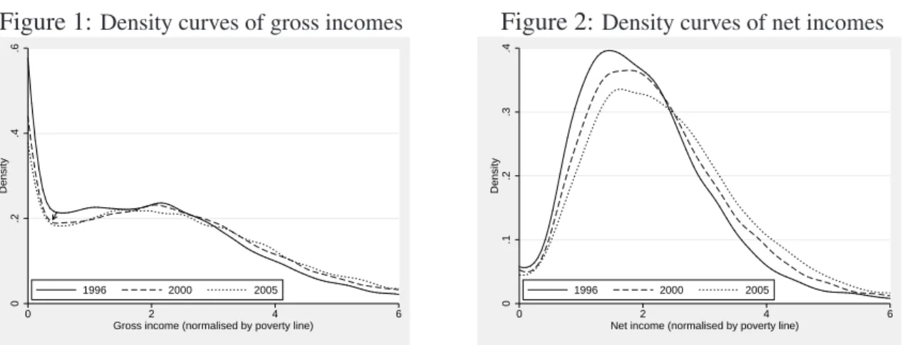
A useful method to have a complete picture on the form of distribution of wealth is to draw its density function. For this purpose, the Gaussian corrected boundary kernel estimator is used to estimate density functions. Indeed, with the usual kernel estimation of the density of incomes close to the minimum bound will be biased. This is explained mainly by the high frequency of population with low or null market income15. In figures (1) and (2), we plot density functions of gross and net income respectively16. This first remark concerns the shift of the density curve of net income to the left side between years of 1996 to 2005. This shift indicates that household wellbeing have increased on average during this period. The other remark concerns the change in shape of the density function of gross income where the latter began less flat. One can recall here that inequality is inversely linked with the kurtosis of
14Statistic Canada codify the total income before taxes by TTINC27 and the after-tax income by ATINC27. 15All estimates reported in this paper are done with Stata, DASP and DAD packages. See also
Araar and Duclos (2007a).
16To simplify the presentation of income values, the unity of income was normalized to equal the poverty
Figure 1: Density curves of gross incomes 0 .2 .4 .6 Density 0 2 4 6
Gross income (normalised by poverty line) 1996 2000 2005
Figure 2: Density curves of net incomes
0 .1 .2 .3 .4 Density 0 2 4 6
Net income (normalised by poverty line) 1996 2000 2005
the distribution17. To clarify this better, for flatter density function, the population size of the poor and rich groups are relatively higher and the expected disparity in income or inequality is high.
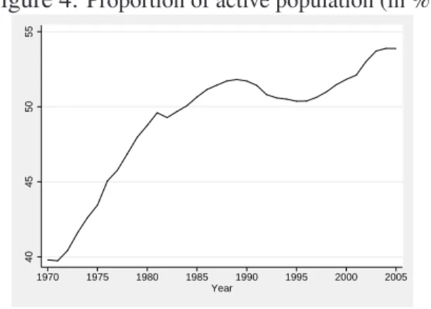
Now we try to shed light on the main factors that can explain the increase in average in-come during the last decade. Before discussing the trend of usual indicators, like the GDP per capita, one must clarify the following idea. Overtime, even if the average returns of alloca-tion of endowments remain constant (real wage for instance), the change in the composialloca-tion of population, expressed by the change in the proportion of active population, may influence the variation in average income. The trend of real GDP, plotted in figure (3), indicates that Canada has experienced a good economic performance during the two last decades. However, the trend of active population rate shows a higher increase in proportion of active population (see figure (4))18. This conclusion is also confirmed by figures (5) and (6), where the expected household size for a given level of gross income has decreased during the last decade. An increase in welfare through the change in the composition of population, or equivalently, a decrease in ratio of dependence may be temporal. The renewal of active population must be perceived as an inter-generational investment to ensure the availability of the adequate size of active population over the long term. Governmental policies proposed to increase the birth rate, and migration policies must be well designed to fill the expected gap in active population for the next generations.
3.4 The evolution of social class structure
As reported through the presentation of the theoretical framework in section 2, we focus on three main social classes, which are the poor, the middle and the rich social class. To fix the thresholds of poor class, we use the Low Income Cut-Offs (LICOs) as the poverty line. One can recall here that LICOs are by far Statistic Canada’s most established and widely recognized approach to estimating low income cut-offs. In short, a LICO is an income threshold below which a household will likely devote a larger share of its total expenditures
17A high kurtosis distribution has a sharper “peak” and flatter “tails”, while a low kurtosis distribution has a
more rounded peak with wider “shoulders”.
Figure 3: Real growth domestic product −5 0 5 10 1970 1975 1980 1985 1990 1995 2000 2005 Year
Figure 4: Proportion of active population (in %)
40 45 50 55 1970 1975 1980 1985 1990 1995 2000 2005 Year
Figure 5:Expected household size according to
household gross income
1.5
2
2.5
3
3.5
Expected household size
10000 20000 30000 40000 50000 60000 Household gross income
1996 2000 2005
Figure 6: Expected equivalent household size
according to household gross income
1.2
1.4
1.6
1.8
2
Expected equivalent household size
10000 20000 30000 40000 50000 60000 Household gross income
1996 2000 2005
on the necessities of food, shelter and clothing than the average household. The approach is essentially to estimate an income threshold at which families are expected to spend 20 percent more than the average household expenditures on food, shelter and clothing. To fix a comfortable richness line, we assume that the latter is three times the poverty line. One can consider that these social class thresholds are estimated with the absolute approach, since they are not based explicitly on some estimated statistics at a population level, like the average income.
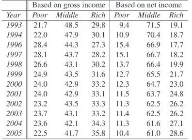
Table 1: Population share of the social classes (Absolute approach)
Based on gross income Based on net income
Year Poor Middle Rich Poor Middle Rich
1993 21.7 48.5 29.8 9.4 71.5 19.1 1994 22.0 47.9 30.1 10.9 70.4 18.7 1996 28.4 44.3 27.3 15.4 66.9 17.7 1997 28.1 43.7 28.2 15.1 66.7 18.2 1998 26.6 43.1 30.2 13.7 66.4 19.9 1999 24.9 43.5 31.6 12.7 65.5 21.7 2000 24.0 42.9 33.2 12.3 64.7 23.0 2001 24.0 42.9 33.1 11.5 63.7 24.8 2002 23.2 43.5 33.3 11.3 62.5 26.2 2003 23.7 43.1 33.2 11.4 62.5 26.2 2004 23.6 42.1 34.3 11.3 61.6 27.1 2005 22.5 41.7 35.8 10.4 61.0 28.6
The population shares of social classes are presented in table (1). From the table, one can conclude that:
- In chronic way and starting from the year of 1996, there is a clear tendency in the decrease of proportions of poor and middle classes at the detriment to that of the rich class.
- Redistributive policies, have contributed widely in maintaining the desired structure of social classes. This is reflected by the important decrease in poverty and the increase in middle class by about 50%, when the net income is used.
- The tendency of increase in rich class at the detriment of the middle one is confirmed with gross and net incomes.
Based on the last conclusion, one can argue that social classes may be appropriately defined under the relative criteria to determine a threshold. Indeed, the average income can increase overtime and preferences of the population may change. This process can imply a more expensive lifestyle. To assess the evolution of the three main social classes with relative approach, we assume that poverty line simply equals half of average income. In addition, we assume that the lower bound for the rich class is equal to twice the average of income. Based on results of table (2), the increase of the rich class is confirmed again with the relative approach.
Table 2: Population share of social classes (Relative approach)
Based on gross income Based on net income
Year Poor Middle Rich Poor Middle Rich
1993 25.9 66.0 8.1 12.4 83.6 4.0 1994 26.1 65.8 8.1 13.8 82.3 3.9 1996 31.6 59.1 9.3 17.3 77.7 5.0 1997 31.4 59.2 9.4 17.3 77.6 5.0 1998 31.0 59.9 9.1 16.9 78.0 5.1 1999 29.6 61.4 9.0 16.6 78.5 4.9 2000 29.2 61.7 9.2 16.8 78.1 5.1 2001 29.4 61.5 9.0 16.9 77.9 5.2 2002 29.0 62.0 9.0 16.8 78.2 5.0 2003 29.4 61.5 9.1 17.1 77.9 5.0 2004 29.4 61.2 9.3 17.3 77.5 5.2 2005 29.2 61.4 9.4 17.0 77.8 5.2
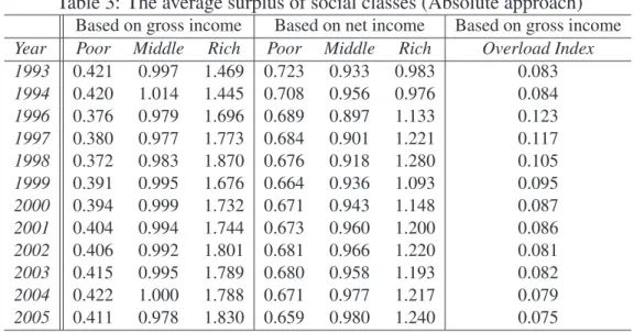
Now we turn to check how wellbeing of social classes has evolved overtime. For this purpose, we estimate the surplus index (α = 1) for each social class by taking into account only its population size19. Starting from results of table (3), one can conclude the following:
Table 3: The average surplus of social classes (Absolute approach)
Based on gross income Based on net income Based on gross income
Year Poor Middle Rich Poor Middle Rich Overload Index
1993 0.421 0.997 1.469 0.723 0.933 0.983 0.083 1994 0.420 1.014 1.445 0.708 0.956 0.976 0.084 1996 0.376 0.979 1.696 0.689 0.897 1.133 0.123 1997 0.380 0.977 1.773 0.684 0.901 1.221 0.117 1998 0.372 0.983 1.870 0.676 0.918 1.280 0.105 1999 0.391 0.995 1.676 0.664 0.936 1.093 0.095 2000 0.394 0.999 1.732 0.671 0.943 1.148 0.087 2001 0.404 0.994 1.744 0.673 0.960 1.200 0.086 2002 0.406 0.992 1.801 0.681 0.966 1.220 0.081 2003 0.415 0.995 1.789 0.680 0.958 1.193 0.082 2004 0.422 1.000 1.788 0.671 0.977 1.217 0.079 2005 0.411 0.978 1.830 0.659 0.980 1.240 0.075
- Based on gross income, the average income of the poor group has increased slightly while that of the middle class has remained practically constant between 1996 and 2005. However, the main increase in wealth was aspired by the rich class.
19The average surplus for each social class is estimated with its population size instead of that of total
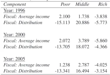
Table 4: Decomposition of variation in social class indices
(Fiscal System: Xt→ Nt)
Component Poor Middle Rich
Year: 1996
Fiscal: Average income 2.100 1.738 -3.838
Fiscal: Distribution -15.113 20.886 -5.773
Year: 2000
Fiscal: Average income 2.072 3.789 -5.860
Fiscal: Distribution -13.705 18.072 -4.366
Year: 2005
Fiscal: Average income 1.238 2.787 -4.025
Fiscal: Distribution -13.341 16.494 -3.154
Table 5: Decomposition of variation in social class indices
Component Poor Middle Rich
Period: 1996-2000
Market: Average income -2.186 -3.846 6.033
Market: Distribution -2.261 2.424 -0.162 ∆I(X, α) -4.448 -1.423 5.870 ∆CµX→µN -0.028 2.051 -2.023 ∆CπX→πN 1.407 -2.815 1.407 ∆I(N, α) -3.068 -2.186 5.255 Period: 2000-2005
Market: Average income -0.941 -1.706 2.647
Market: Distribution -0.497 0.545 -0.048 ∆I(X, α) -1.438 -1.161 2.599 ∆CµX→µN -0.834 -1.002 1.836 ∆CπX→πN 0.365 -1.577 1.212 ∆I(N, α) -1.907 -3.740 5.647 Period: 1996-2005
Market: Average income -3.210 -5.429 8.639
Market: Distribution -2.676 2.846 -0.170
∆I(X, α) -5.886 -2.584 8.469
∆CµX→µN -0.862 1.049 -0.187
∆CπX→πN 1.772 -4.392 2.620
- Based on net income, the surplus of the poor has decreased overtime whereas those of the middle and rich classes have increased. The increase in the surplus of the rich class continues to be the more pronounced.
- The overload index, which equals to the ratio between the poor gap and the non poor surplus, has decreased overtime. This indicates, inter alias, an increase in the tax base system and in the potential of tax income revenues.
To show how variations in average income and distribution between gross and net income affect social class indices, we present in table (4) the contribution of each of these two com-ponents. It is well known that a part of fiscal revenue is not distributed directly to households, but used to finance other public services. The expected decrease in average of available in-come has contributed in increasing the poor and middle class in detriment of the rich one. However, one must be prudent about this conclusion since the benefit of public goods is not entered.
In table (5), we present results of decomposition of social indices based on net income. Starting from these results, one can conclude the following:
- For all retained periods, the market growth component has contributed in reducing population share of the poor and middle classes and has increased the rich class.
- Distribution through market forces has contributed in increasing of population share of the middle class. One can judge this aspect socially and economically efficient.
- As indicated in table (4), the fiscal system contributes in decreasing the poor class. However, results reported in table (5), show that the rate of decrease is slowly reduced. This is explained, inter alias, by the improvement in distribution of wellbeing during the last years and where the inequality has significantly decreased20.
- The last important remark concerns the non neglected effect of market forces on social class structure (see results of (5)). This conclusion suggests that, in the short-run, one must give more attention to the evolvement of market forces and does not rely mainly on the fiscal system to correct the distribution of wealth.
3.5 The trend of inequality and polarization
As reported in the theoretical framework section, inequality indices are useful to summa-rize all information about disparity in incomes with one index. Indeed, this process allows us to assess the evolution of inequality overtime. In table (6), we present the trend of inequality in gross and net incomes for the period between 1993 and 2005. Starting from results of this table, one can conclude the following:
- Since 1996, inequality in gross income has continuously decreased until 2005. This may be attributed mainly to the good economic performance during this period, and the economic environment has helped the reinsertion of poor group to economic activity sphere.
20Note that even of redistributive policies of the fiscal system remain unchanged overtime, a decreases in
inequality of gross income decreases the redistributive effect of the fiscal system. This aspect is well discussed in section 2.6.
- Overtime, the impact of the fiscal system seems to be linear and depends mainly on the shape of the distribution of gross income. This conclusion is based, in part, on the stable impact of the fiscal system on inequality. This may be attributed to the rigidity of adjustment of the fiscal system overtime or to its delay to respond to the punctual economic shocks.
Table 6: The trend of inequality in Canada
Gini index Between provinces inequality
Gross Net Change Gross Net Change
Year income income in (%) income income in (%)
1993 0.392 0.270 -31.2 0.055 0.041 -26.7 1994 0.391 0.274 -29.8 0.050 0.037 -24.4 1996 0.449 0.307 -31.6 0.053 0.038 -27.4 1997 0.452 0.312 -30.9 0.056 0.041 -26.9 1998 0.452 0.313 -30.7 0.061 0.046 -24.5 1999 0.427 0.300 -29.7 0.050 0.040 -19.3 2000 0.424 0.303 -28.7 0.048 0.040 -17.3 2001 0.425 0.304 -28.6 0.048 0.036 -23.9 2002 0.424 0.304 -28.2 0.041 0.029 -29.3 2003 0.424 0.304 -28.3 0.042 0.031 -27.0 2004 0.422 0.304 -27.9 0.042 0.030 -28.8 2005 0.422 0.305 -27.9 0.045 0.032 -29.8
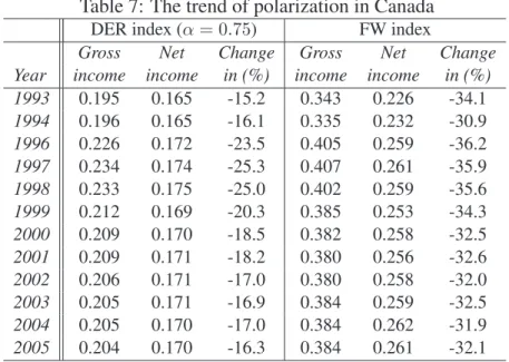
Table 7: The trend of polarization in Canada
DER index (α = 0.75) FW index
Gross Net Change Gross Net Change
Year income income in (%) income income in (%)
1993 0.195 0.165 -15.2 0.343 0.226 -34.1 1994 0.196 0.165 -16.1 0.335 0.232 -30.9 1996 0.226 0.172 -23.5 0.405 0.259 -36.2 1997 0.234 0.174 -25.3 0.407 0.261 -35.9 1998 0.233 0.175 -25.0 0.402 0.259 -35.6 1999 0.212 0.169 -20.3 0.385 0.253 -34.3 2000 0.209 0.170 -18.5 0.382 0.258 -32.5 2001 0.209 0.171 -18.2 0.380 0.256 -32.6 2002 0.206 0.171 -17.0 0.380 0.258 -32.0 2003 0.205 0.171 -16.9 0.384 0.259 -32.5 2004 0.205 0.170 -17.0 0.384 0.262 -31.9 2005 0.204 0.170 -16.3 0.384 0.261 -32.1
The other interesting investigation for study of inequality inequality is about the conver-gence of average incomes across provinces in Canada. It is well known that inequality indices may be decomposed across population groups21. The Gini index can be decomposed into
within and between group components. The component between-group is inversely linked to the level of convergence of incomes across groups. Usually, to estimate the between-group inequality, we use a counterfactual vector of incomes where each individual have the aver-age income of its group. The larger the decrease in between-group inequality overtime, the greater is the convergence of incomes across provinces. The between provinces inequality of gross and net incomes are reported in table (6). In general, one can remark a clear tendency of convergence of incomes across provinces in Canada. In addition, the fiscal system has accelerated this convergence.
Now, we focus on the evolution of polarization in Canada and how governmental inter-ventions, through taxes and transfers, have reduced its level. In table (7), we present the trend of the DER polarization index for gross and net incomes. Polarization in gross incomes has decreased considerably between 1997 and 2000. The registered decrease in polarization of net income was low overtime. Using theFoster and Wolfson (1992) bipolarisation index, we arrive practically to the same conclusion. Obviously, the fiscal system has contributed widely in reducing bipolarization of net income, and where the average reduction is about the third bipolarization of gross income.
3.6 The evolution of progressivity of the fiscal system
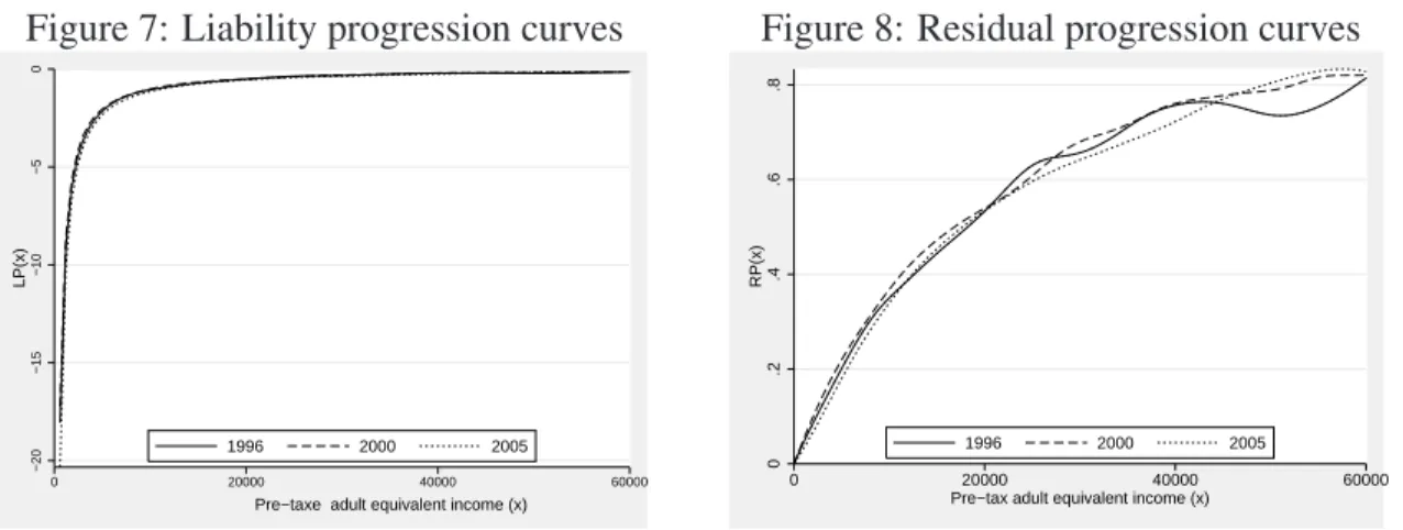
Has the Canadian fiscal system become more progressive over the last years? To respond to this question, we use the local and global measurements of progressivity. To test the local progressivity of fiscal system, we show in figures7and8the liability and the residual progression curves22. Starting from these results, one can confirm the local progressivity of Canadian fiscal system. With the liability approach and when of per equivalent adult gross income is lower than 20 000 $CAN, the local progressivity is more pronounced for the year 2005.
Figure 7: Liability progression curves
−20 −15 −10 −5 0 LP(x) 0 20000 40000 60000
Pre−taxe adult equivalent income (x) 1996 2000 2005
Figure 8: Residual progression curves
0 .2 .4 .6 .8 RP(x) 0 20000 40000 60000
Pre−tax adult equivalent income (x) 1996 2000 2005
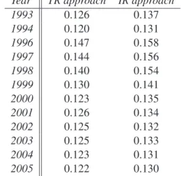
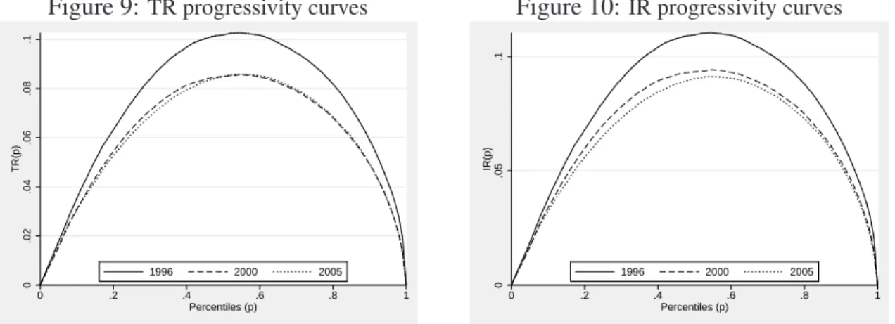
Now we estimate the progressivity with the global approach. Starting from results re-ported in table8, as well as, those of figures9and10, one can conclude that the fiscal system
22Note that all estimates were done using the Stata package DASP (Araar and Duclos (2007a)). Local
pro-gressivity curves require, inter alias, the use of the non parametric and the derivative non parametric regressions. For more information, contact the author.
was progressive for each of the studied years. The other remark, that one can draw promptly, is the apparent decrease in progressivity of the fiscal system during the last few years, and this by comparing between estimated progressive indices across years. However, one must be prudent on this conclusion. As indicated in theoretical framework section, the absence of the common support of comparison for the progressivity in the fiscal system across years may mitigate our conclusion. Otherwise, progressivity indices cannot be compared with the change in distribution of gross income from one year to another. To remedy to this, we use the year of 2005 as the base pre-tax income year (gross income in our case) and we estimate the expected net income of 2005 based on the fiscal system of 1996 or 2000. To estimate the counterfactual vector of net incomes of 2005, based on fiscal system of a given prece-dent year, we use the locally linear non parametric estimation approach. It follows that, for each value of gross income found in the survey of 2005, we use information on gross and net incomes of the given precedent year to estimate the expected net income. Obviously, this procedure does not give us any information about the expected local variability of net income. Fortunately, this local variability does not affect estimation of progressivity indices. This is explained mainly by the fact that concentration indices -curves- weight locally the average level of tax or net income according to the rank of the gross income. Results concerning the evolution of the fiscal system’s progressivity, when the base pre-tax income year is that of 2005, are reported in table9and figures11and12. Among the most important conclusions, that one can draw, is the increase of progressivity of the fiscal system in 2005 with the TR approach. The other remark concerns the non neglected impact of change in pre-tax income on progressivity indices.
Table 8: The evolution of fiscal system progressivity in Canada
Year TR approach IR approach
1993 0.126 0.137 1994 0.120 0.131 1996 0.147 0.158 1997 0.144 0.156 1998 0.140 0.154 1999 0.130 0.141 2000 0.123 0.135 2001 0.126 0.134 2002 0.125 0.132 2003 0.125 0.133 2004 0.123 0.131 2005 0.122 0.130
Figure 9:TR progressivity curves 0 .02 .04 .06 .08 .1 TR(p) 0 .2 .4 .6 .8 1 Percentiles (p) 1996 2000 2005
Figure 10: IR progressivity curves
0 .05 .1 IR(p) 0 .2 .4 .6 .8 1 Percentiles (p) 1996 2000 2005
Table 9: The evolution of fiscal system progressivity in Canada Base pre-tax income year: 2005
TR approach IR approach
1996 0.1152 0.1300
2000 0.1161 0.1296
2005 0.1222 0.1299
Figure 11: TR progressivity curves Base pre-tax income year: 2005
0 .02 .04 .06 .08 TR(p) 0 .2 .4 .6 .8 1 Percentiles (p) 1996 2000 2005
Figure 12: IR progressivity curves Base pre-tax income year: 2005
0 .02 .04 .06 .08 .1 IR(p) 0 .2 .4 .6 .8 1 Percentiles (p) 1996 2000 2005
4 Conclusion
This paper focuses on the evolution of the social class structure in Canada, as well as, in the experienced change in inequality, polarization and progressivity in the fiscal system between 1993 and 2005. In addition to the macroeconomic performance criteria, one has to assess and to analyze the experienced change in distribution of wealth overtime. It has been argued that a macroeconomic performance may help increase wellbeing in average, but not guarantee a more equitable distribution of wealth. Overtime, there are many factors that can contribute to the reshaping of the distribution of income. In addition to economic growth, other factors like market forces, population endowments and fiscal system measures can influence largely the distribution of wealth. In Canada, both the fiscal system and social programs are crucial tools for reducing disparities in income. In general, with these govern-mental interventions, the deprived group receive a special treatment. Indeed, the government ensures a worthy standard of living to the socially excluded group and help them be rein-serted into the economic activity sphere. For instance, the government can finance programs of re-qualification and attribute valuable financial advantages to join the labour market or to be maintained in it.
To assess the evolution of the different distributive phenomena, we use the national repre-sentative SLID survey and we choose net income as the indicator of wellbeing for Canadian households. For the normalization of income at the individual level, we adopt conventional and widely accepted methods in publications of Statistic Canada. Developed and most up-dated distributive tools are used to assess and to understand better some links between the studied distributive phenomena. The following summarizes the main conclusions of this study:
• Household wellbeing has registered a significant increase during the last decade. How-ever, one can notice the important change in active population rate and a decrease in the dependency ratio, which help improve the welfare in average during the last few years.
• The social class structure in Canada has registered a significant change during the last decade. When the absolute approach is adopted to define social classes, we find that the population share of the rich class has increased by about 10% of total population. The redistributive market component has contributed to a sharper increase in wellbeing of this class. In addition, these factors have contributed to reduce the population share of the poor class and to increase that of the middle class.
• While inequality in gross income has a registered continuous decrease between 1996 and 2005, inequality in net income has remained practically constant, except its small increase in 1996/97. More importantly, the follow-ups of the evolution of the compo-nent inter-province inequality enabled us to conclude for the chronic convergence of incomes across provinces in Canada.
• Results concerning the trend of polarization or bipolarisation in distribution of incomes are not far from those of inequality, and where the main reduction is registered with gross income.
• As expected, the fiscal system has contributed largely in increasing the middle class and decreasing the poor group. Its redistributive effect has also decreased substantially the level of inequality and polarization.
• For each year, progressivity of fiscal system was confirmed by two methodological approaches. For the comparison of progressivity across time, the main conclusion con-cerns the non neglected impact of change in pre-tax income on progressivity indices. The other is the increase in the progressivity of fiscal system in 2005, when the same base pre-tax income is used for different periods.
Note finally that conclusions and remarks drawn in this study can help policymakers un-dertake optimal strategic policies to enhance the social performance. The other contribution of this study is on the development of methods to assess the progressivity of the fiscal sys-tem. Our method of distributive analysis carried at the Canadian level can be replicated at provincial level. Finally, this study can inspire future works to investigate and to improve the distributive methods developed in this study.
References
ARAAR, A. (1999): “Social classes and distributive indices,” Conference: Cr´efa, Uni-versit´e Laval, D´epartment d’ ´Economique.
——— (2002): “L’impact des variations des prix sur les niveaux d’in´egalit´e et de bien-ˆetre: Une application a la Pologne durant la p´eriode de transition. (With English summary.),” L’Actualit´e Economique/Revue D’Analyse Economique, 78, 221–42. ——— (2003): “The Shapley Value,” Tech. rep., SISERA TRAINING WORKSHOP
ON POVERTY DYNAMICS, Universit´e Laval, CIRP ´EE and PEP, http://www.pep-net.org/NEW-PEP/Group/PMMA/pmma-train/files/I-Shapley-Araar.pdf.
——— (2005): “Social classes and distributive indices: Illustration with the LIS data,” Mimeo, Universit´e Laval, PEP and CIRP ´EE, http://132.203.59.36/DAD/pdf files/soc class.pdf.
——— (2006): “On the Decomposition of the Gini Coefficient: an Exact Approach, with an Illustration Using Cameroonian Data,” Cahiers de recherche 0602, CIRPEE. ——— (2008): “On the Decomposition of Polarization Indices: Illustrations with
Chi-nese and Nigerian Household Surveys,” Cahiers de recherche 0806, CIRPEE. ARAAR, A.ANDT. T. AWOYEMI(2006): “Poverty and Inequality Nexus: Illustrations
with Nigerian Data,” Cahier de recherche 0638, CIRPEE.
ARAAR, A.ANDJ.-Y. DUCLOS(2003): “An Atkinson-Gini family of social evaluation functions,” Economics Bulletin, 3, 1–16.
——— (2007a): “DASP: Distributive Analysis Stata Package,” PEP, CIRP ´EE and World Bank, Universit Laval.
——— (2007b): “Poverty and Inequality Components: a Micro Framework,” Cahier de recherche 0735, CIRPEE.
CHEN, S. AND M. RAVALLION (2001): “How Did the World’s Poorest Fare in the
1990s?” Review of Income and Wealth, 47, 283–300.
DATT, G. AND M. RAVALLION (1992): “Growth and Redistribution Components of
Changes in Poverty Muasures: a Decomposition with Applications to Brazil and India in the 1980’s,” Journal of Development Economics, 38, 275–295.
DUCLOS, J.-Y.ANDA. ARAAR(2006): Poverty and Equity Measurement, Policy, and
Estimation with DAD, Berlin and Ottawa: Springer and IDRC.
DUCLOS, J.-Y., J. ESTEBAN, ANDD. RAY(2004): “Polarization: Concepts, Measure-ment, Estimation,” Econometrica, 72, 1737–1772.
ESTEBAN, J.AND D. RAY(1994): “On the Measurement of Polarization,”
Economet-rica, 62, 819–51.
FOSTER, J., J. GREER, AND E. THORBECKE (1984): “A Class of Decomposable
Poverty Measures,” Econometrica, 52, 761–776.
FOSTER, J. AND M. WOLFSON (1992): “Polarization and the Decline of the Middle
HURST, C. E. (2007): Social Inequality Forms, Causes, and Consequences, MA. KAKWANI, N. (1977): “Measurement of Tax Progressivity: An International
Compari-son,” Economic Journal, 87, 71–80.
——— (1993): “Poverty and Economic Growth with Application to Cote d’Ivoire,”
Review of Income and Wealth, 39, 121–39.
——— (1997): “On measuring Growth and Inequality Components of Changes in Poverty with Application to Thailand,” Discussion paper 97/16, The University of New South Wales.
KASTEN, R., F. S.O. E. T. (1994): Trends in Federal Tax Progressivity, In J. Slemrod.
KESSELMAN, J. R. AND R. CHEUNG (2004): “Tax Incidence, Progressivity, and
In-equality in Canada,” Canadian Tax Journal, 52, 709.
LAMBERT, P.AND R. ARONSON(1993): “Inequality Decomposition Analysis and the
Gini Coefficient Revisited,” Economic Journal, 103, 1221–27.
MARX, K. (1861-3): Theories of Surplus Value, International Publishers.
MUSGRAVE, R.ANDT. THIN(1948): “Income Tax Progression 1929-48,” The Journal
of Political Economy, 56, 498–514.
OECD (2007): “Dataset: Country statistical profilese,” Statistics, Organisation for Eco-nomic Co-operation and Development.
RAVALLION, M. AND B. BIDANI(1994): “How Robust Is a Poverty Profile?” World
Bank Economic Review, 8, 75–102.
RODRGUEZ, J. G. (2004): “Measuring polarization, inequality, welfare and poverty,” Tech. rep.
ROWNTREE, S. (1901): Poverty, a study of town life, London: MacMillan.
SHORROCKS, A. (1999): “Decomposition procedures for distributional analysis: A
unified framework based on the Shapley value,” Tech. rep., University of Essex. STATCAN (2007): “Survey of Labour and Income Dynamics (SLID) - A Survey
Overview,” Tech. rep.
THORESEN, T. O. (2002): “Reduced Tax Progressivity in Norway in the Nineties The Effect from Tax Changes,” Discussion Papers 335, Research Department of Statis-tics Norway.
WEBER, M. (1964): The Theory of Social and Economic Organization. ——— (1978): Economy and Society, Berkeley.
ZHANG, X. AND R. KANBUR (2001): “What Difference Do Polarisation Measures