2014 — Contribution to improving the accuracy of serial robots

(1)

ÉCOLE DE TECHNOLOGIE SUPÉRIEURE UNIVERSITÉ DU QUÉBEC

MANUSCRIPT-BASED THESIS PRESENTED TO ÉCOLE DE TECHNOLOGIE SUPÉRIEURE

IN PARTIAL FULFILLMENT OF THE REQUIREMENTS FOR THE DEGREE OF

DOCTOR OF PHILOSOPHY Ph. D.

PAR

Albert NUBIOLA BATLLE

CONTRIBUTION TO IMPROVING THE ACCURACY OF SERIAL ROBOTS

(2)

It is forbidden to reproduce, save or share the content of this document either in whole or in parts. The reader who wishes to print or save this document on any media must first get the permission of the author.

(3)

BOARD OF EXAMINERS

THIS THESIS HAS BEEN EVALUATED BY THE FOLLOWING BOARD OF EXAMINERS

M. Ilian A. Bonev, directeur de thèse

Département de génie de la production automatisée, École de technologie supérieure

M. Antoine Tahan, président du jury

Département de génie mécanique, École de technologie supérieure

M. Pascal Bigras, membre du jury

Département de génie de la production automatisée, École de technologie supérieure

M. René Mayer, examinateur externe

Département de génie mécanique, École Polytechnique de Montréal

THIS THESIS WAS PRESENTED AND DEFENDED IN THE PRESENCE OF A BOARD OF EXAMINERS AND PUBLIC

DECEMBER 17TH 2014

(4)

(5)

ACKNOWLEDGEMENTS

I would like to thank my supervisor Prof. Ilian Bonev for being such a great advisor. I could always count on his support and brilliant ideas his dedication greatly inspired me. There has always been the chance to work on new projects with new companies and state of the art equipment in the CoRo laboratory.

I thank the automation team at Pratt & Whitney Canada for giving me the opportunity to have an industrial experience in the manufacturing of airplane engines at the Longueuil plant. Thanks to Canam Hoang, David Lafortune, Pierre-Phillippe Poirier, Mélanie Tremblay, Yuwen Li and François Dupras, from whom I did not just learn about industrial manufacturing but also about the Quebecoise culture.

I would also like to thank AV&R Global, especially Tommy Gagnon, for trusting our robot calibration methods to calibrate their Fanuc robots.

I am grateful to my colleagues at the CoRo, especially Yanick Noiseux, Mohamed Slamani, Yousef Babazadeh, Andy Yen and Ahmed Joubair, who assisted me in many different ways.

I thank La Caixa d’Estalvis i Pensions de Barcelona, “la Caixa” for funding my studies. I also thank le Fonds québecois de la recherché sur la nature et les technologies (FQRNT) and the Natural sciences and engineering research council of Canada (NSERC) for their funding.

Last but not least, I thank my family for their support. Their constant love, support and encouragement were essential to complete this work. My parents and my three brothers have always been nearby despite the geographical distance.

(6)

(7)

CONTRIBUTION À L’AMÉLIORATION DE LA PRÉCISION DES ROBOTS SÉRIELS

RÉSUMÉ

Le but de la présente étude est de contribuer à l’amélioration de la précision absolue des robots manipulateurs sériels à six degrés de liberté. Ces méthodes consistent à identifier les valeurs des paramètres du robot, en vue d’améliorer la correspondance entre le robot réel et le modèle mathématique utilisé par son contrôleur. Le modèle du robot étalonné ajoute des paramètres d’erreur au modèle nominal; ces paramètres correspondent aux erreurs géométriques et au comportement élastique du robot.

Les méthodes développées se concentrent sur les systèmes de mesure à faible coût. Le premier travail fait une comparaison entre un étalonnage robot fait avec un laser de poursuite (« laser tracker ») et une caméra stéréo (MMT optique). L’amélioration de la précision est validée en utilisant une barre à billes pour chacune des deux méthodes d’étalonnage. Le résultat de l’étalonnage est le même pour les deux méthodes tandis que le prix d’un laser de poursuite est plus que deux fois le prix d’une caméra stéréo. La méthode est validée avec un robot ABB IRB 120, un laser de poursuite Faro ION, et une caméra stéréo C-Track de Creaform. Une barre à billes Renishaw QC20-W permet de valider la précision obtenue de manière indépendante.

Un système de mesure innovateur qui permet de mesurer un ensemble de poses est décrit à la deuxième partie de la thèse. Ce dispositif est basé sur une approche d’hexapode connu (la plateforme Stewart-Gough). Une plaque doit s’attacher à la base du robot et une autre à l’outil; chaque plaque contient trois supports magnétiques. Ce système permet de mesurer 144 poses de l’outil par rapport au support de la base en prenant six mesures de la barre à billes pour chaque pose. La précision tridimensionnelle de ce dispositif est 3.2 fois la précision de la barre à billes QC20-W, soit ± 0.003 mm. Dans la troisième partie de cette thèse, on utilise ce nouvel système de mesure 6D pour faire un étalonnage absolue d’un robot. Le robot est étalonné dans 61 configurations et la précision de positionnement absolue est validée avec un laser de poursuite Faro dans environ 10,000 configurations de robot. L’erreur de distance moyenne est améliorée de 1.062 mm à 0.400 mm dans 50 millions de pairs de mesures dans tout l’espace de travail du robot. A titre comparatif, le robot est aussi étalonné avec un laser de poursuite et la précision est validée dans les mêmes 10,000 configurations.

(8)

(9)

CONTRIBUTION TO IMPROVING THE ACCURACY OF SERIAL ROBOTS

ABSTRACT

The goal of the present study is to improve the accuracy of six-revolute industrial robots using calibration methods. These methods identify the values of the calibrated robot model to improve the correspondence between the real robot and the mathematical model used in its controller. The calibrated robot model adds error parameters to the nominal model, which correspond to the geometric errors of the robot as well as the stiffness behavior of the robot. The developed methods focus on using low cost measurement equipment. For instance, the first work makes a comparison between a robot calibration performed using a laser tracker and a stereo camera (MMT optique) separately. The accuracy performance is validated using a telescoping ballbar for each of the two methods. While the calibration result is the same for both methods, the price of a laser tracker is more than twice the price of a stereo camera. The method is tested using an ABB IRB120 robot, a Faro ION laser tracker, and a Creaform C-Track stereo camera to calibrate the robot. A Renishaw QC20-W ballbar is used to validate the accuracy.

A novel measurement system to measure a set of poses is described in the second work. The device is an extension of a known approach using an hexapod (a Stewart-Gough platform). One fixture is attached to the robot base and the other to the robot end-effector, each having three magnetic cups. By taking six ballbar measurements at a time, it is possible to measure 144 poses of the triangular fixture attached to the robot end-effector with respect to the base fixture. The position accuracy of the device is 3.2 times the accuracy of the QC20-W ballbar: ± 0.003 mm. An absolute robot calibration using this novel 6D measurement system is performed in the third work of this thesis. The robot is calibrated in 61 configurations and the absolute position accuracy of the robot after calibration is validated with a Faro laser tracker in about 10,000 robot configurations. The mean distance error is improved from 1.062 mm to 0.400 mm in 50 million pairs of measurements throughout the complete robot workspace. To allow a comparison, the robot is also calibrated using the laser tracker and the robot accuracy validated in the same 10,000 robot configurations.

(10)

(11)

TABLE OF CONTENTS

Page

INTRODUCTION ...1

CHAPTER 1 LITTERATURE REVIEW ...3

1.1 Absolute vs. relative calibration ...5

1.2 Open-loop vs. closed-loop calibration ...5

1.3 Robot calibration process ...6

1.3.1 Level-1 calibration ... 7

1.4 Kinematic modeling ...8

1.5 Inverse kinematics computation ...9

1.5.1 Analytical ... 10 1.5.2 Numeric... 10 1.6 Optimization algorithms ...12 1.6.1 Line-search methods ... 13 1.6.2 Trust-region method... 13 1.6.3 Nelder-Mead ... 13

1.7 Commercial solutions for robot calibration ...14

1.7.1 Dynalog ... 14

1.7.2 Nikon Metrology ... 15

1.7.3 Teconsult ... 17

1.7.4 Wiest AG ... 18

1.7.5 American Robot Corporation ... 19

1.8 Recent calibration results reported in the literature ...21

CHAPTER 2 COMPARISON OF TWO CALIBRATION METHODS FOR A SMALL INDUSTRIAL ROBOT BASED ON AN OPTICAL CMM AND A LASER TRACKER ...25

2.1 Introduction ...25

2.2 Experimental setups ...28

2.2.1 Triangular artifact ... 33

2.2.2 Spatial artifact ... 34

2.3 Robot kinematic model ...36

2.4 Analysis of non kinematic robot behavior ...38

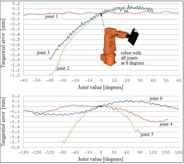
2.4.1 Axis analysis with the laser tracker ... 38

2.4.2 Stiffness model... 41

2.5 Calibration...42

2.5.1 System linearization ... 43

2.5.2 Observability ... 44

2.5.3 Laser tracker and triangular artifact (setup 1) ... 45

(12)

2.5.5 C-Track and spatial artifact (setup 3) ... 46

2.6 Results ...46

2.6.1 Analysis of the measurement devices ... 47

2.6.2 Validation using the laser tracker and the C-Track ... 49

2.6.3 Validation using a telescopic ballbar ... 54

2.7 Conclusions ...58

2.8 Acknowledgments...59

CHAPTER 3 A NEW METHOD FOR MEASURING A LARGE SET OF POSES WITH A SINGLE TELESCOPING BALLBAR ...61

3.2 Choosing the Optimal Hexapod Design for our 6D Measurement Device ...66

3.3 Direct Kinematics of our Hexapod Design ...74

3.4 Calculating the Accuracy of the 6D Measurement Device ...77

3.5 Experimental Validation ...78

3.6 Conclusion ...83

3.7 Acknowledgements ...84

CHAPTER 4 ABSOLUTE ROBOT CALIBRATION WITH A SINGLE TELESCOPING BALLBAR ...85

4.2 Experimental Setup and Description of Measurement System ...88

4.3 Robot Calibration Model and Parameter Identification Procedure ...96

4.4 Experimental Results ...99

4.5 Conclusions ...107

4.6 Acknowledgements ...108

GENERAL CONCLUSION ...109

FUTURE WORK ...111

ANNEX I CALIBRATED ROBOT MODEL ...113

(13)

LIST OF TABLES

Page Table 2.1 Pose of the base frame with respect to the world frame with six error

parameters ...36

Table 2.2 Complete D-H M (Craig, 1986) robot model with 25 error parameters ...36

Table 2.3 Ranges of motion for each joint for the test, the results of which are shown in Figure 2.6 ...39

Table 2.4 Masses and centers of gravity of each robot link in our model ...42

Table 2.5 Distance errors for the C-Track and the laser tracker with respect to the CMM ...49

Table 2.6 Robot base errors obtained with the laser tracker and the triangular artifact ...50

Table 2.7 Robot model obtained with the laser tracker and the triangular artifact ...51

Table 2.8 Robot base errors obtained with the C-Track and the triangular artifact ...52

Table 2.9 Robot model obtained with the C-Track and the triangular artifact ...52

Table 2.10 Robot base errors obtained with the C-Track and spatial artifact ...53

Table 2.11 Robot model obtained with the C-Track and the spatial artifact ...54

Table 2.12 Summary of ballbar results obtained using the triangular artifact ...56

Table 2.13 Summary of ballbar results obtained using the spatial artifact ...58

Table 3.1 Measurement uncertainties for each of the three tool attachment points in the four DKP solutions shown in Figure 3.5 ...78

Table 3.2 Errors for the 39 robotic configurations tested ...81

Table 3.3 Errors for 15 additional tool poses measured using the FaroArm ...83

Table 4.1 Robot calibration model used (25 error parameters) ...97

Table 4.2 Estimated masses and centers of gravity of each robot link for Fanuc LR Mate 200iC robot ...97

Table 4.3 Absolute position errors (in mm) in 9,905 robot configurations ...104

(14)

Table 4.5 Distance errors (in mm) for all pairs of the 9,905 robot configurations ...106 Table 4.6 Distance errors (in mm) for all pairs of the 3,672 front/up

(15)

LIST OF FIGURES

Page

Figure 1.1 Robot calibration using the CompuGauge device ...15

Figure 1.2 Nikon K-Series optical CMM ...16

Figure 1.3 Rosy measurement device ...17

Figure 1.4 Robot calibration using LaserLAB ...19

Figure 1.5 MasterCal calibration setup ...20

Figure 2.1 Experimental setup for calibrating the robot with FARO’s ION laser tracker 31 Figure 2.2 Experimental setup for calibrating the robot with Creaform’s C-Track and the triangular artifact: (a) overall setup; (b) close-up showing the back side of the triangular artifact and the fifteen retro-reflective targets on the robot’s base ..32

Figure 2.3 Experimental setup for calibrating the robot with Creaform’s C-Track and the spatial artifact ...33

Figure 2.4 The spatial artifact during photogrammetry ...35

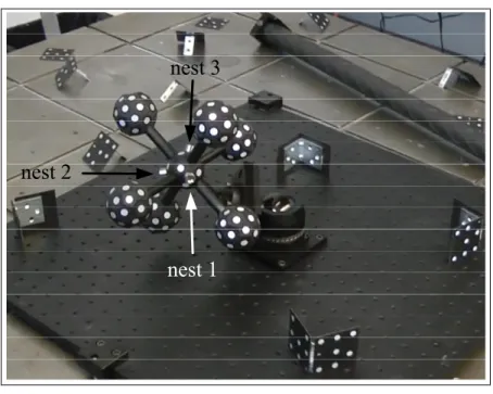
Figure 2.5 The positions of the three magnetic nests with respect to Φ6 are measured directly ...38

Figure 2.6 Tangential errors measured when rotating a single joint ...40

Figure 2.7 Calibration and validation positions using (a) the laser tracker and the triangular artifact (setup 1); (b) the C-Track and the triangular artifact (setup 2); (c) the C-Track and the spatial artifact (setup 3) ...45

Figure 2.8 Accuracy validation of the C-Track and laser tracker on the CMM ...48

Figure 2.9 Histogram of position errors using the laser tracker and the triangular artifact ...50

Figure 2.10 Histogram of position errors using the C-Track and the triangular artifact. ....51

Figure 2.11 Histogram of position errors using the C-Track and the spatial artifact ...53

Figure 2.12 Measuring distance accuracy with a Renishaw telescopic ballbar ...55

Figure 2.13 Results for the path with the ballbar attached to nest 1 of the triangular artifact ...55

(16)

Figure 2.14 Results for the path with the ballbar attached to nest 2 of the

triangular artifact ...56

Figure 2.15 Results for the path with the ballbar attached to nest 1 of the spatial artifact ...57

Figure 2.16 Results for the path with the ballbar attached to nest 3 of the spatial artifact ...57

Figure 3.1 A CMM of hexapod design (courtesy of Lapic, Russian Federation) ...64

Figure 3.2 Early designs using telescoping ballbars in a hexapod arrangement for pose measurements ...64

Figure 3.3 The main components of the standard W kit from Renishaw: (1) QC20-W ballbar; (2) center pivot assembly; (3) Zerodur calibrator; (4) setting ball; (5) magnetic cup; (6-8) 50 mm, 150 mm and 300 mm extension bars ...67

Figure 3.4 (a) A general 6-6 hexapod and (b) the most common example of a 3-3 hexapod ...67

Figure 3.5 Four of the eight possible DKP solutions for the 112212331_{hexapod ...71}

Figure 3.6 The 72 different tool poses that can be measured using our device (18 of these, marked with a white cross, are superfluous) ...72

Figure 3.7 Position and orientation distances between the tool reference frames of each pairing of the 72 measurable poses shown in Figure 3.6 ...74

Figure 3.8 A schematic representation of the 112212331 hexapod design ...76

Figure 3.9 Measuring the base and tool distances as well as the leg distances in a given robot configuration ...79

Figure 3.10 The 22 tool poses measurable using our device for a single setup of the base fixture. In 17 of these poses (not identified here), the robot can be positioned with two wrist configurations. ...82

Figure 4.1 Experimental setup for measuring the pose of the robot end-effector ...89

Figure 4.2 Illustration of one of the 3-3 hexapod designs used ...90

Figure 4.3 The four feasible assembly configurations for the 231 3-3 hexapod ...91

Figure 4.4 Relationship between the initial and corrected world reference frames ...94

(17)

Figure 4.6 Robot configurations used for calibration (continues) ...102 Figure 4.7 Absolute position error for the two steps of the calibration process ...105 Figure 4.8 Distance errors between the two types of measured configurations ...106

(18)

(19)

LIST OF ABBREVIATIONS AND ACRONYMS

CAD Computer assisted design

CMM Coordinate measuring machine

CNC Computer numerical control

CoRo Control and robotics laboratory

CPC Complete and parametrically continuous

CRIAQ Consortium for research and innovation in aerospace in Québec D-H Denavit-Hartenberg

D-H M Denavit-Hartenberg modified, as defined in (Craig, 1986)

DBB Double-ball bar

DOF Degree of freedom EE End-effector

ETS École de Technologie Supérieure

HMI Human-machine interface

IDP Inverse displacement problem

ISO International organization for standardization MMT Machine à mesurer tridimensionnelle

NSERC Natural sciences and engineering research council of Canada

OLP Off-line programming

TCP Tool center point

SMR Spherically-mounted reflector

(20)

s(θ) sin(θ) c(θ) cos(θ) si sin(qi)

ci cos(qi)

Trans(x,y,z) Geometrical translation {x,y,z}

Rot(v,θ) Geometrical rotation of θ around unit vector v

RMS Root mean square

(21)

LIST OF SYMBOLS AND UNITS OF MEASUREMENT kg Kilogram g Gram N Newton Hz Herz (measures/second) s Second ms Millisecond

º Degree (“deg” is used in some figures) rad Radian

m Meter mm Millimeter µm Micrometer

Nm Newton-meter (torque)

(22)

(23)

INTRODUCTION

Industrial robots are mainly conceived and used in repetitive applications, therefore, they successfully perform tasks programmed in teach mode. Some examples of typical robot applications are pick and place operations, welding, painting, machine tending, palletizing and assembly. These types of applications do not require high robot accuracy levels as long as the robot path is manually taught; in this case, the accuracy is the same as the repeatability. However, there is an increasing demand of applications where the robot should be programmed through off-line programming (OLP). Robot paths can be more sophisticated by programming a robot using simulator software; therefore, the robot can be used in a more extended number of applications, such as inspection, machining, drilling or composite fiber placement. Furthermore, the production of the robot does not need to be interrupted. Even though robots are highly repeatable, their accuracy is far below their repeatability. Therefore, the accuracy of a robot can be improved through robot calibration.

The demand of industrial robots having better accuracy and reduced cost has been constantly growing in the past decade, especially in the aerospace sector (Summers, 2005). Today, most industrial robot manufacturers and a few service providers offer robot calibration services. Furthermore, many industrial robot manufacturers now adopt the ISO 9283 norm, which was not the case a decade ago (Greenway, 2000; Schröer, 1999). Nevertheless, the only information regarding the positioning performance of an industrial robot continues to be a single measure specified as “positioning performance according to ISO 9283”, which actually refers to the average unidirectional position repeatability and accuracy at five poses obtained from thirty cycles. A few additional performance measures might be obtained from certain robot manufacturers (e.g., found in the product manual of the robot), such as linear path repeatability and linear path accuracy, but even this information is highly insufficient and impossible to use if we want to compare two robots manufactured by different companies.

(24)

The absolute accuracy of a robot is not usually specified by its manufacturer. The accuracy of a robot is not important as long as the robot path is manually taught. In this case we only want the robot to be repeatable. However, in off-line programming the accuracy becomes an important issue since positions are defined in a virtual space from an absolute or relative coordinate system. There are also some industrial applications where a robot is used as a measurement system, for example, when the robot holds a touch probe to locate the part to be processed; in this case, the accuracy of the robot becomes the accuracy of the measurement system.

It is required to study the forward kinematic model to improve robot accuracy. Starting with the nominal kinematic model of a robot and adding error parameters we can find a mathematical model that represents the robot better than the nominal kinematic model. This improved model must make the robot more accurate, improving position and orientation errors.

This work focuses on finding new robot calibration methods for six-revolute industrial serial robots. The calibration methods must give good accuracy results while maintaining the cost of the measurement equipment as low as possible. The calibrated robot model used only physically meaningful parameters into account, which allows for extrapolation if the robot environment is modified, such as the robot payload or the inclination angle of the robot.

This thesis is organized in four chapters. Chapter 1 presents a literature review on robot calibration. Chapter 2 compares two different measurement systems to be used in robot calibration: a laser tracker and a stereo camera. A novel six-dimensional (6D) measurement system is introduced in Chapter 3. This measurement system can measure the pose of 144 configurations by using only one telescoping ballbar, very accurate 6D measurements can be obtained with low-cost one-dimensional equipment. Finally, Chapter 4 performs a robot calibration using the novel 6D measurement system. Chapters 2, 3 and 4 have been published as articles in scientific journals (A Nubiola et al., 2013; A. Nubiola and Bonev, 2014; Albert Nubiola et al., 2013).

(25)

CHAPTER 1

LITTERATURE REVIEW

This chapter describes the calibration methods established in the literature, more precisely the robot calibration process, the three levels of robot calibration, the kinematic representation used for calibrated robots and the optimization methods used for parameter identification. The most relevant commercial solutions for robot calibration are also mentioned in this chapter, as well as some recent robot calibration results reported in literature.

Industrial robots propose an interesting alternative to dedicated machines. A robot should be calibrated to get the best production performance. Robots require high accuracy levels to perform advanced operations; for example, an accurate robot is much more suitable to perform tasks that have been programmed off-line. Furthermore, if we have a stiffness model of the robot, we could compensate any forces applied to the robot end-effector (EE), such as in a machining operation (Dumas et al., 2011).

Although robot calibration has been studied for more than two decades, the theory remains the same as in the early 1980s (Barker, 1983). What is different nowadays is that robots are better built (i.e., their repeatability is greater) and the sources of errors, with respect to their nominal models, are slightly different. Measurement equipment is also better, i.e., more accurate, though certainly not much more affordable. The mathematical models that used to work for robots a decade or two ago are no longer optimal for today’s robots. Furthermore, the accuracy required today in some potential robot applications is much higher than a couple decades ago.

Nowadays, two measures are commonly used for describing the positioning performance of industrial robots: repeatability and accuracy.

(26)

Loosely speaking, pose repeatability is the ability of a robot to repeatedly return to the same pose. In robotics, the ISO 9283 defines the repeatability term and it is used by most industrial robot manufacturers. The ISO norm actually refers to unidirectional repeatability only, which is the ability to return to the same pose coming from the same direction, thus minimizing the effect of backlash. Multidirectional repeatability can be twice the unidirectional repeatability or even worse.

Repeatability can be improved by either high-precision gear trains (as in most Staübli robots), by placing high-resolution encoders at the output of the gear trains or using direct-drive motors (as in some SCARA robots). However, all of these solutions raise the manufacturing cost of an industrial robot.

Loosely speaking, volumetric accuracy (also called absolute accuracy) is the ability of a robot to attain a pose with respect to a reference frame. Since identifying such a reference frame is not always simple with a robot (for example, it might require using a touch probe), accuracy is most typically tested in relative measurements, e.g., distance accuracy is the ability of the robot to displace its tool center point (TCP) a prescribed distance.

Robot accuracy is affected by the same factors as multidirectional repeatability; it is obviously lower bounded by the multidirectional repeatability of the robot. Accuracy is influenced mostly by geometric inaccuracies and elasticity, present in both the links and the transmissions. Fortunately, these two types of errors can be modeled to some extent in the robot calibration process (Abderrahim et al., 2007).

There are five factors that cause robot errors (Andrew Liou et al., 1993; Karan and Vukobratovic, 1994): environmental (such as temperature or the warm-up process), parametric (for example, kinematic parameter variation due to manufacturing and assembly errors, influence of dynamic parameters, friction and other nonlinearities, including hysteresis and backlash), measurement (resolution and discretisation of joint position

(27)

sensors), computational (computer round-off and steady-state control errors) and application (such as installation errors).

Robot calibration can be divided into several categories and subcategories. The following two sections compare an absolute calibration with a relative calibration and an open-loop with a closed-loop calibration respectively.

1.1 Absolute vs. relative calibration

An absolute calibration allows attaining accurate positions with respect to a physically measurable frame. A relative calibration disregards the actual location of the robot base whereas an absolute calibration takes into account where the robot base is placed. In other words, if we want more than one robot to share the same coordinate system they need to be “absolute” calibrated to agree with the same “absolute” reference frame (also called world frame). An absolute calibration is not needed if we are positioning the robot relatively to a local frame (also called object or user frame), so we need a tool, such as a touch probe, which allows us to locate objects in the robot working space. An absolute calibration needs six more parameters than a relative calibration because we need to represent the relative frame with respect to an absolute frame.

1.2 Open-loop vs. closed-loop calibration

In short, a closed-loop calibration uses the robot encoders as a measurement system and an object of precisely known geometry is used as a reference to perform calibration. Whenever we use a measurement system to directly measure the pose of the robot tool, such as a laser tracker, we apply an open-loop calibration. On the other hand, a closed-loop method is used if the robot tool is constrained to lie on a reference object of precisely known geometry. This method only needs a switch such as a touch probe to detect the contact with an obstacle, when the robot is placed at the contact position the joint values given by the encoders are registered.

(28)

We can find several methods used for measuring robot position as the measurement system technology has improved a lot in the past two decades. Some examples of open-loop methods are acoustic sensors (Stone and Sanderson, 1987), visual systems such as cameras (Meng and Zhuang, 2001; Puskorius and Feldkamp, 1987), coordinate measuring machines (CMM) (M R Driels et al., 1993; Lightcap et al., 2008; B. W. Mooring and Padavala, 1989) and, of course, laser tracking systems (Shirinzadeh, 1998). There has also been some research work that allows a laser tracking system to identify the 6 parameters of the tool pose (Vincze et al., 1994).

One example of closed-loop calibration is the MasterCal commercial product from American Robot, where the constraints are the diameter of two spheres and the distance between their centers. Other examples are the use of planar constraints (Ikits and Hollerbach, 1997), or point constraints (Meggiolaro et al., 2000) or (Houde, 2006).

1.3 Robot calibration process

A robot calibration process is divided in four sequential steps (Roth et al., 1987): modeling, measurement, identification and correction. The modeling step consists of finding a model that represents the real robot through its kinematics equations. It is the robot model that takes into account the various error parameters to calculate the pose with respect to the robot joints. Data from the real robot allows generating the equations that the identification algorithm will use to find an improved robot model, better than the nominal kinematic model.

It is important to differentiate tool calibration from robot calibration. We may usually calibrate the tool at the same time as the robot is being calibrated. However, a separate tool calibration must be taken into account when the tool which we want to be precisely positioned is not the one that we used during calibration.

Through robot calibration we obtain a new model that can represent the real robot better than the nominal model. The nominal model is the one used in the robot controller, and for decoupled robots, with the so-called inline wrists (the axes 4, 5 and 6 intersect at one point),

(29)

the inverse kinematics of the nominal model is simple and can be solved analytically. A robot calibration implies error parameters inserted to design parameters (nominal model) that represent the real source of errors. These parameters are called error parameters which must be found by the calibration method.

Although optimization algorithms are not primordial when calibrating a robot, they can be very helpful in improving precision if they are used appropriately. Some optimization algorithms are described in Section 1.6.

A robot calibration can be divided in three levels (B. Mooring et al., 1991). The calibration level will be defined depending on which real error parameters the model represents.

1.3.1 Level-1 calibration

The goal in a level-1 calibration is to properly define the relationship between the desired joint position (θd) and the real joint position (θr). In the nominal model we consider that they

are both the same, however, in real life we have a more complex relationship where the real joint positions are a function of the desired joints _θ_r =f ( )_θ_d . This relationship may be difficult to obtain properly but we can reach good approximations with linear functions in a reduced workspace. The most basic linear relationship would be:

1 0

r k d k

θ = θ + . (1.1)

Where k0 is the offset constant and is close to zero whereas k1 is the proportionality constant. A level-1 calibration is also known as a “joint level” calibration.

A level-2 model is defined as a robot kinematic calibration. That means that some, or all, of the geometric parameters are modelled. Distance and angle offsets are added as error parameters to the robot’s nominal design. At the same time, a level-2 model can include a level-1 model to model the behavior of the joints.

(30)

When an entire kinematic calibration is needed we can identify the robot’s joint axes and extract the kinematic parameters placing frames that relate each joint axis with the next one. The calibration needs the virtual joint axes in the same absolute reference frame and the geometry of the end-effector referred to the robot’s tool frame. To extract the virtual axes we must set the robot at the home position, and moved each joint one by one taking measures by intervals (B. Mooring et al., 1991). A circle that minimizes the sum of error squares can fit these points. From these circles we can extract the axes.

This idea was developed independently by several researchers. Once we have the virtual robot axes there are basically two methods to extract the kinematic parameters: Stone’s method and Sklar’s method (B. Mooring et al., 1991). Stone’s method (Stone and Sanderson, 1987) finds the kinematic model known as “S-model” (6 parameters per joint) and Sklar’s method finds the D-H representation of the robot placing the frames at the appropriate place. Both methods are explained and compared in (B. Mooring et al., 1991).

A level-3 model takes into account any non-geometrical error sources. Non-geometrical sources of errors can be stiffness, friction, backlash, dynamical parameters, etc. A level-3 model usually contains level-2 and level-1 error parameters. Most common robot calibrations include a full kinematic calibration (level-2) and sometimes a few parameters describing the stiffness of the robot’s arm (level-3) (Aoyagi et al., 2010; Dumas et al., 2011; Lightcap et al., 2008; Marie et al., 2013; Saund and DeVlieg, 2013).

1.4 Kinematic modeling

The best-known four-parameter representation model in robotics is the one given by Denavit-Hartenberg (Denavit and Denavit-Hartenberg, 1955). This so-called D-H notation is widely used in robotics. There is also a very similar and well-known representation commonly referred to as Denavit-Hartenberg Modified (D-H M) notation, which is the notation defined by (Craig,

(31)

1986). Both representations model the kinematic parameters of the robot, the main difference remains on the order of the geometrical transformations. Both make a translation and rotation over the X and Z axis (one translation and one rotation each). The D-H notation starts with a rotation about the X axis while the D-H M notation starts with a rotation about the Z axis (translation and rotation around the same axis can be alternated with no final effect). For a detailed review of the direct kinematic modeling, see (Craig, 1986; Paul, 1981; Slotine and Asada, 1992).

The D-H notation has been used by several researchers for robot calibration, such as (Veitschegger and Wu, 1987; Wei and De Ma, 1993). However, this representation introduces singularity problems when two consecutive axes are parallel or almost parallel (Hayati and Mirmirani, 1985). The complete and parametrically continuous (CPC) model eliminates this problem (Hanqi Zhuang et al., 1992) by representing the relationship between each link with three translations and one rotation instead of two translations and two rotations. Similarly, the product of exponentials (POE) representation makes the error parameters vary smoothly with changes in joint axes so that no special descriptions are required when consecutive joint axes are close to parallel (Brockett, 1984; I.-M. Chen et al., 1997; Okamura and Park, 1996; Park, 1994).

Finally, other types of representations have also been used. There is a five-parameter representation for prismatic joints (Hayati and Mirmirani, 1985) or even six parameter representation (Stone and Sanderson, 1987), but if we insert more than four parameters the calibration problem becomes redundant.

1.5 Inverse kinematics computation

Solving the inverse kinematics of a decoupled 6R serial robot is straightforward, and it can be achieved using analytical methods (Craig, 1986). For a calibrated robot it is also necessary to find a way to calculate the inverse solution for a given model and pose, also known as the inverse displacement problem (IDP). Modifying the robot model’s parameters within the robot controller is usually difficult or impossible depending on the complexity of the model

(32)

chosen. Therefore, the best solution is to use fake targets which modify the real coordinates by a slightly modified target which takes into account the nominal model calculations of the robot controller.

Once the robot model is defined, we should describe how we are going to solve the inverse solution of the calibrated robot. There are many solutions available in the literature but not all of them are suitable to all robot models. Depending on what level of calibration we use we will need one or another inverse solution. Inverse kinematics calculation can be divided in two main types: analytical and numerical.

1.5.1 Analytical

We should use an analytical solution to the IDP for the calibrated robot model whenever possible. However, as we add error parameters to our basic kinematic model, the simplifications that we can usually do on a nominal model can no longer be done due to the complexity of the equations. A semi-algebraic method to solve the IDP was found to simplify a level-2 model (geometric model) into a 16th degree polynomial (Angeles, 2007), at this point numerical computations are needed to obtain the solution. To the best of our knowledge, there has not been any work that obtains an analytical solution for a level-3 calibration.

1.5.2 Numeric

Iterative solutions offer an easy way to solve complex problems at a cost of computation time. Obviously, when an algebraic solution cannot be found, an iterative method must be applied. This numerical method approaches the solution at each iteration. In some cases, the robot model can be seen as a black box that can only compute the forward calculation obtaining the pose given the joint angles. Industrial robots have path motion planners that cut a path (trajectory) into a large number of targets and the inverse solution must be applied to each point of the path.

(33)

Any generic optimization method could be applied to solve the IDP, such as the optimization algorithms used to obtain the modelled error parameters; however, better optimization methods exist as the problem is more specific. In the worst case we have to find as many parameters as the number of joints that the robot has.

Numerical methods can be divided in three types (N. Chen and Parker, 1994): (1) Newton-Raphson methods, (2) predictor-corrector type algorithms, and (3) optimization techniques using the formulation of a scalar cost function. Examples of the first method can be found in (Angeles, 1985), where a modified Newton-Gauss method is used. Such methods involve the computation of the Jacobian matrix. A comparison between Newton-Raphson methods and predictor-corrector-type algorithms is provided in (Gupta and Kazerounian, 1985), where the authors conclude that the latter are faster.

An example of a predictor-corrector algorithm is given in (Tsai and Orin, 1987). This type of method often requires a large number of iterations, and does not always converge. Some of these algorithms also require computation of the Jacobian matrix, like the algorithm proposed in (Goldenberg et al., 1987), which combines a predictor-corrector type of algorithm with a least-squares optimization technique, or the closed-loop method (Siciliano, 2009) where the inverse kinematic problem is solved as a control problem for a simple dynamic system. However, optimization techniques are usually complex, and several iterations are needed to achieve a solution.

Two approaches for level-2 calibrations are proposed in (Vuskovic, 1989) using the nominal inverse kinematics. However, the solution becomes complex when the number of error parameters increases. The resolution of a nonlinear programming problem is divided into two phases in (L. C. T. Wang and Chen, 1991) for greater efficiency.

The amount of computing time to solve the IDP is greatly improved in (N. Chen and Parker, 1994) by calculating a so-called pose shift by iteratively adding and subtracting computed poses based on a truncated-series expansion of the desired pose. However, we realized that

(34)

their method could be further improved by using pose multiplications based on a geometric principle, instead of adding and subtracting the poses of the truncated-series expansion of the desired pose.

Finally, we introduced a new geometrical approach to solving the IDP (Albert Nubiola and Bonev, 2014). Similar to (N. Chen and Parker, 1994), our method does not need the computation of the Jacobian matrix or derivatives of any kind. Up to eight solutions can be obtained from the sixteen possible solutions of the IDP.

1.6 Optimization algorithms

Once we have defined a robot model we must obtain the error parameters by taking measurements from the real robot. The most suitable optimization algorithms for most types of robot models are nonlinear and unconstrained. Plenty of algorithms, more precisely the genetic algorithm (K. Wang, 2009), represent small variations of kinematic parameters and the end-effector error is represented by a fitness function. At every generation, a population of parameters is created and brings a better solution to replace the existing solution. This technique does not need computationally expensive calculations such as the inverse of the Jacobian matrix.

Other alternatives for robot calibration have been reported in the literature, such as the Taguchi method (Judd and Knasinski, 2002; Karan and Vukobratovic, 1994) or (Judd and Knasinski, 2002). The work (H Zhuang and Roth, 2002), for example, uses different methods to identify the unknown error parameters (similar to the CPC model).

Optimization methods can be mainly classified in two types: line-search methods and trust-region methods. We can also describe an optimization method that differs from the first two types: the Nelder-Mead method.

(35)

1.6.1 Line-search methods

There are different types of line-search optimization methods. They differ by the way they compute the line search direction. We can find the following line-search methods: Newton’s method, gradient descent method and Quasi-Newton method (Bonnans and Lemaréchal, 2006).

Newton’s method is also known as Newton-Raphson method. Newton algorithms are implemented in Matlab’s optimization toolbox in the functions fsolve, fminunc and lsqcurvefit.

1.6.2 Trust-region method

The trust-region method is also known as restricted step method. It handles the case when the Jacobian matrix is singular and it is useful when the initial guess is far from a local minimum. This method approximates the objective function with a simpler function in the neighborhood of the solution at each iteration.

Trust region methods are dual to line search methods. The first one chooses a step size before a search direction while the second one chooses a search direction and then a step size.

1.6.3 Nelder-Mead

This optimization algorithm was proposed by John Nelder and Roger Mead (Nelder and Mead, 1965). It is also called simplex method (a non linear method that is different from the known linear simplex method). It evaluates the objective function over a polytope in the parameter space. If we have two parameters, the polytope is a triangle as we are in a 2D plane. If there are n-dimensions, we have an (n+1)-sided polytope.

The algorithm compares these n+1 points and deletes the worst one. The worst point is replaced by its reflection through the remaining points in the polytope. This algorithm is

(36)

simple and does not need gradient information but it takes time to achieve a solution when we have more than six variables. This method is also implemented in Matlab’s optimization toolbox, in the function fminsearch.

1.7 Commercial solutions for robot calibration

Most robot manufacturers offer calibration as an option. For example, in the case of ABB Robotics, most of its robots can be calibrated at the factory with the CalibWare software for about C$2,000 per robot, using a Leica laser tracker, a single SMR (Spherically-mounted reflector) and around 40 error parameters. However, ABB does not offer an on-site calibration service, unlike KUKA. ABB also has a tool to improve resolver offsets due to motor exchange and maintenance: the calibration pendulum.

As an example, L-3 MAS Canada at Mirabel use Motoman industrial robots and have them calibrated on-site by Motoman, who use a third-party calibration software (from Dynalog). Similarly, Messier-Dowty at Mirabel use three KUKA industrial robots and have them calibrated on-site by KUKA.

1.7.1 Dynalog

Dynalog is a Detroit-based privately held company founded in 1990 by Dr. Pierre De Smet, then professor at Wayne State University. Dynalog is the most renowned expert in robot calibration. While the company offers several products improving the accuracy of industrial robots, the two of greatest interest are the CompuGauge hardware and the DynaCal software. The first is a 3D (x, y ,z) measurement device based on four string encoders that intersect at one point. Dynalog claims that the volumetric accuracy of the CompuGauge measurement device is 0.150 mm and its repeatability is 0.020 mm inside a cubic working volume of side 1.5 m. The price of this device is at least US$9,000, but while not expensive, the device is quite bulky and difficult to install.

(37)

Figure 1.1 Robot calibration using the CompuGauge device1

DynaCal is the software for robot calibration that accepts measurement data from the CompuGauge device or from any other precise 3D or 6D measurement device. The software and the adapters for fixing SMRs are sold to industry for more than US$40,000. While all demonstrations of DynaCal show the use of a laser tracker and a single SMR, it seems that DynaCal can also work with three SMRs, thus calibrating the complete pose of the end-effector.

Dynalog also has a specific patented product to calibrate robots that is used for part inspections (De Smet, 2001). Dynalog offers a complete robot library which makes it possible to calibrate many robots from different brands.

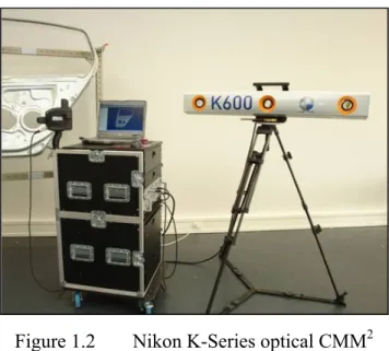
1.7.2 Nikon Metrology

Metris International Holding was purchased by Nikon in 2009 to create Nikon Metrology. Metris, a market leader for CMM based laser scanning, was founded in 1995 and is

(38)

headquartered in Belgium. In 2005, Metris acquired Belgium-based Krypton, which was specializing in robot calibration since 1989.

Nikon Metrology offers a large number of metrology systems, but the two that are of particular interest to us are the K-Series Optical CMM and the ROCAL software. The first one is basically a three-camera system that measures the spatial coordinates of up to 256 infrared LEDs (thus, it can provide 6D measurements). The volumetric accuracy of the K-Series Optical CMM is better than 0.090 mm which is close to the laser tracker accuracy and certainly sufficient for robot calibration. Its price is about C$80,000.

Figure 1.2 Nikon K-Series optical CMM2

ROCAL is software for robot calibration, very similar to Dynalog’s DynaCal. It seems that some of the differences are a better integration with some robot brands (KUKA, Mitsubishi and COMAU) and the software’s incompatibility with measurement devices other than the K-Series Optical CMM. The software also relies on complete pose measurement data.

2 http://www.nikonmetrology.com/var/ezwebin_site/storage/images/products/portable-measuring/optical-cmm/k-series-optical-cmm/179510-2-eng-GB/K-Series-Optical-CMM.jpg

(39)

1.7.3 Teconsult

Teconsult is a Germany based university spin-off offering a unique 3D optional measurement device called ROSY and the robot calibration software that goes with it. Teconsult was founded by Prof. Lukas Beyer in 1999. ROSY is a measuring tool based on a videometric principle with two digital CCD cameras. Two cameras are used in order to get a more uniform volumetric accuracy. The tool is attached to the robot flange and is used to measure, with respect to the robot flange frame, the spatial position of the center of a small white ceramic ball that is fixed with respect to the robot’s base. The ROSY device itself is calibrated on a CMM before shipment.

The calibration procedure consists of reorienting the tool and measuring the position of the ball for 40 different poses (Beyer and Wulfsberg, 2004), for a single location of the ceramic ball. According to reference (Beyer and Wulfsberg, 2004) the volumetric accuracy of ROSY is ±0.020 mm inside a spherical measurement range of ±2 mm. However, ROSY is offered in several different sizes, and there is no information whether that volumetric accuracy is for a small or for a large ROSY device.

Figure 1.3 Rosy measurement device3

(40)

ROSY is rather bulky and requires removal of the end-effector from the robot. Furthermore, it requires several relatively thick cables to be run along the robot arm. A complete ROSY system for tool, base and robot calibration is about €17,500 (US$21,000). However, it seems that Teconsult does not offer any means to calculate the inverse kinematics.

1.7.4 Wiest AG

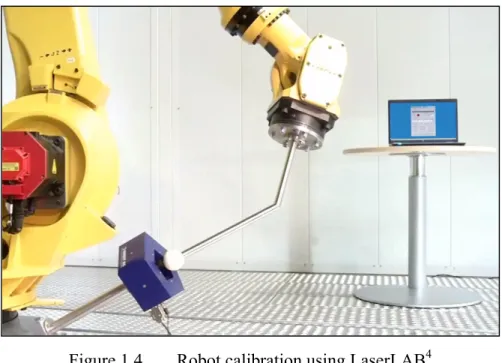
Wiest is another Germany based university spin-off offering another unique 3D optical measurement device called LaserLAB and the robot calibration software that goes with it. Wiest AG was founded by Dr. Ulrich Wiest who has been working in the field of robot calibration since 1996 (he obtained his doctoral degree in 2001).

LaserLAB is patent-pending (Wiest, 2003) and consists of five small-range one-dimensional laser distance sensors mounted to a common frame and with their lasers intersecting at a common point. A ball is attached to the end-effector of the robot while the LaserLAB device is stationary. By measuring the five distances to the ball (when the center of the ball is approximately at the lasers intersecting point), the spatial coordinate of the center of the ball with respect to the LaserLAB are determined. The repeatability of the LaserLAB is ±0.020 mm, while its volumetric accuracy is better than ±0.100 mm (typically ±0.035 mm), inside a measurement range of 39.5 mm × 38.5 mm × 36.5 mm.

(41)

Figure 1.4 Robot calibration using LaserLAB4

One disadvantage of the LaserLAB is the high likelihood of the sphere colliding with the measurement device while the robot is re-oriented. Furthermore, the only way to measure with a wide range of robot configurations is to use extension rods of different lengths at the end of which a sphere is mounted, rendering that solution practically inconvenient and therefore realistically inaccurate.

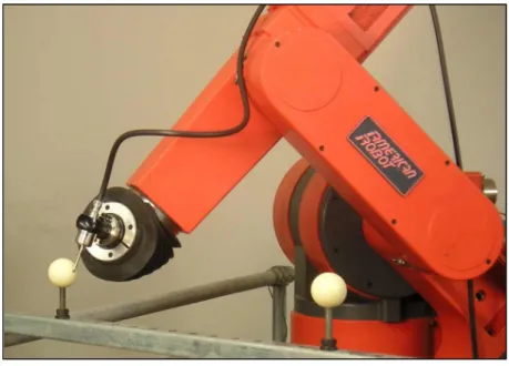
1.7.5 American Robot Corporation

American Robot Corporation (ARC) is a US company based in Pittsburg, Pennsylvania. ARC was established in 1982 and is a manufacturer of industrial robot controllers, industrial robots, and automation systems. It has three major product lines, the Universal Robot Controller, the Merlin articulated six axis robot, and the Gantry 3000 modular gantry robot. ARC also offers a robot calibration software called MasterCal, which makes use of a standard touch probe attached to the flange of a robot and two fixed precision balls separated by a precisely known distance.

(42)

Figure 1.5 MasterCal calibration setup5

The MasterCal calibration procedure was invented and patented by Mr. Wally Hoppe (Hoppe, 2011), a Group Leader and Senior Research Engineer at the University of Dayton Research Institute in Ohio, USA. The basic concept for Mr. Hoppe’s calibration method is an extension of (Meggiolaro et al., 2000), where a single ball-in-socket mechanism was used. Mr. Hoppe’s institution had a huge military contract for robot inspection of aircraft engines and this is how he ended up devising a robot calibration method (he no longer works in robotics). In the course of the patent application, he eventually came across some inventions that are pretty close to this one, although he worked with his lawyer to demonstrate that they do not infringe. The closest method to his invention is by ABB (Snell, 1997). That method uses a single large-diameter precision ball of known diameter and a touch probe. Another very close invention is (Knoll and Kovacs, 2001), which is very general and does not give a lot of detail.

(43)

1.8 Recent calibration results reported in the literature

Research in robot calibration has always been focused on level-2 and level-3 calibrations. A typical example of a level-3 calibration using a stiffness model is (Lightcap et al., 2008), that applies a torsional spring model to represent the flexibility of the harmonic drives by physically meaningful parameters, this model takes into account the flexibility caused by the end-effector. The model improves the mean / maximum error values from 1.77 mm / 4.0 mm to 0.55 mm / 0.92 mm for a Mitsubishi PA10-6CE when loaded at 44 N (validated with only ten measurements on a CMM). This method is more simple than the one proposed in (Khalil and Besnard, 2002) as it does not need the computation of the generalized Jacobian. Also (Caenen and Angue, 1990) represented the angular deformation caused by gravity force. A similar method exists dealing with joint angle dependent errors (Jang et al., 2001).

An example of a kinematic calibration is given in (Ye et al., 2006), where an absolute calibration was performed to an IRB 2400/L with a Faro Xi laser tracker. The mean position error is reduced from 0.963 mm to 0.470 mm for twenty measurements (maximum values are not given, the area of calibration is not given either).

Another example of absolute calibration with a laser tracker is (Newman et al., 2000). Using a Motoman P8 robot, the 27 error parameters from their kinematic model are identified by measuring 367 targets moving each axis separately. The kinematic model that gave best results (for a validation of 21 measurements) corresponds to a “circle-point” algorithm that improves the RMS error from 3.595 mm to 2.524 mm.

We can also mention the work performed by (Bai et al., 2003) that uses a modified CPC model (MCPC) (H Zhuang et al., 1993) to improve the kinematics of a PUMA 560 with 30 error parameters and a laser tracker measurement system. Using 25 measures for parameter identification and 15 measures for verification they reach a mean position error of 0.1 mm, however, when they use a CMM they find that the same position error is 0.4-0.5 mm. The CPC model avoids the singularities associated with parallel axes.

(44)

Other examples of stiffness kinematic models that do not use meaningful parameters are (Jang et al., 2001; Meggiolaro et al., 2005). As stated by (Lightcap et al., 2008), it is better to use meaningful parameters to be able to extrapolate to unknown charges.

The most recent robot calibration research has been focused on modelling the joint stiffness to improve robotic machining applications (Dumas et al., 2011; Marie et al., 2013; Saund and DeVlieg, 2013; Sornmo et al., 2012). For example, (Marie et al., 2013) use a level-3 model (which they call elasto-geometrical) to improve the robot accuracy in machining, forming or assembly applications. The level-3 model contains 27 geometrical error parameters plus 10 error parameters to model the stiffness behavior of the robot. To test the accuracy performance, a KUKA-IR663 robot is calibrated in 126 poses with a payload of 90 kg using the Nikon K600-10 optical CMM, the poses are distributed in a vertical plane grid. The robot accuracy is validated in another set of 63 poses for a 90 kg load and 60 kg separately, the maximum error accuracy of the robot is improved up to 0.371 mm. The robot calibration is compared to a fuzzy logic calibration in the vertical plane of interest. Using this fuzzy logic calibration the maximum error is improved to 0.183 mm.

Another example that focuses on improving the robot accuracy for machining applications is (Sornmo et al., 2012). In this case, the accuracy is not improved through robot calibration but by using a piezo-actuated high-dynamic micro manipulator and a Keyence laser sensor LK-G87 as a tracking system. This paper focuses on improving the surface roughness after a machining process. The surface roughness is improved by a factor of 2.7 in the best case scenario (from 67.0 µm to 24.5 µm).

We can even find companies that perform robot calibration driving the robot using a custom-made controller. This is the case of Electroimpact (Saund and DeVlieg, 2013), that calibrate a Kuka KR360-2 robot as well as the linear axis replacing the original controller for a Siemens 840Dsl CNC controller.

(45)

Finally, we can find a level-3 calibration using 26 geometrical error parameters plus 4 parameters to model the stiffness of joints 2 to 5 (Albert Nubiola and Bonev, 2013). The ABB IRB 1600-6/1.45 robot is calibrated using a Faro ION laser tracker in 52 configurations using three different targets. The maximum position error of the robot is improved from 2.158 mm to 0.696 mm in 1000 configurations using eight different targets. It is also found that the axis 6 has a peculiar error following a Fourier series, probably due to the gear chain in the robot wrist. In the product documentation of a calibrated ABB IRB 1600-6/1.45, it is stated that the typical mean / maximum positioning accuracy is 0.300 / 0.650 mm. We know from Dr. Torgny Brogardh, scientist at ABB Robotics, that this is validated for one tool target (apparently the same target used for calibration). However, we do not have more information regarding the validation procedure, such as the number of measurement configurations.

(46)

(47)

CHAPTER 2

COMPARISON OF TWO CALIBRATION METHODS FOR A SMALL

INDUSTRIAL ROBOT BASED ON AN OPTICAL CMM AND A LASER TRACKER

Albert Nubiola, Mohamed Slamani, Ahmed Joubair and Ilian A. Bonev, 1100 Notre-Dame Ouest, Montréal, Québec, Canada H3C 1K3

This chapter has been published as an article in Robotica: vol. 32, n° 3 (2014), pp 447-466

Abstract

The absolute accuracy of a small industrial robot is improved using a 30-parameter calibration model. The error model takes into account a full kinematic calibration and five compliance parameters related to the stiffness in joints 2, 3, 4, 5, and 6. The linearization of the Jacobian is performed to iteratively find the modeled error parameters. Two coordinate measurement systems are used independently: a laser tracker and an optical CMM. An optimized end-effector is developed specifically for each measurement system. The robot is calibrated using fewer than 50 configurations and the calibration efficiency validated in 1000 configurations using either the laser tracker or the optical CMM. A telescopic ballbar is also used for validation. The results show that the optical CMM yields slightly better results, even when used with the simple triangular plate end-effector that was developed mainly for the laser tracker.

2.1 Introduction

It is well known that the accuracy of an industrial robot can be improved through a process known as robot calibration (Roth et al., 1987). The first step in this process is to choose a theoretical model that is closer to reality than the nominal model used in the robot controller (e.g. the wrist axes are no longer concurrent and the gearboxes are flexible in the new model). The parameters of this model are then identified by measuring the complete pose or

(48)

partial pose of the robot end-effector in a set of calibration configurations. In practice, the most critical issue is the choice of measurement system, as the latter determines the efficiency and cost of the robot calibration process.

The identification process can be performed using a wide range of commercially available or custom-designed measurement tools, such as a touch probe and a reference artifact (Besnard et al., 2000; Hayati and Mirmirani, 1985), a telescopic ballbar (M.R. Driels, 1993; Juneja and Goldenberg, 1997), a small-range 3D (position) measurement device, such as a camera-based system (Beyer and Wulfsberg, 2004) and acoustic sensors (Stone and Sanderson, 1987), a large-range 3D measurement device (such as a laser tracker (Dumas et al., 2010; Meng and Zhuang, 2001; Albert Nubiola and Bonev, 2013; Puskorius and Feldkamp, 1987) or CMM (M.R. Driels, 1993; Lightcap et al., 2008; B. W. Mooring and Padavala, 1989)) and a 6D (pose) measurement device, such as a camera-based system (Gatla et al., 2007; Meng and Zhuang, 2001; Puskorius and Feldkamp, 1987) or a laser tracker with a 6D probe (Boochs et al., 2010).

To the best of our knowledge, most industrial robot manufacturers who offer calibration as an option use either a laser tracker (one manufactured by Leica, in the case of ABB and FANUC) or a 6D optical CMM (Nikon Metrology’s K-series optical CMM, in the case of KUKA). Furthermore, at least two commercial robot calibration software packages exist, based on 3D or 6D measurement data: DynaCal from Dynalog, and Rocal from Nikon Metrology (both companies based in the US).

In practice, two types of commercially available position/pose measurement tools can be used for calibrating industrial robots: laser trackers (from Leica, FARO, or API) and optical CMMs (from Nikon Metrology, Northern Digital, Metronor, Geodetic Systems, AICON, GOM, or Creaform). Laser trackers are more accurate and have a very large measurement range, but they are highly sensitive to the ambient conditions (e.g. the air currents present in factory hangars) and are extremely expensive (from at least $100,000 US to nearly $200,000 US or more). Laser trackers generally measure the 3D coordinates of a single point at a time,

(49)

but they can also be used to measure the complete pose of the robot end-effector in static conditions, by measuring three SMRs (spherically mounted reflectors), or, in dynamic conditions, by using a special 6D probe for measuring. However, at each moment, a laser tracker measures the position or pose of a single body relative to its own reference frame. Therefore, vibrations of the factory floor can significantly decrease the accuracy to which the position or pose of the robot end-effector is measured with respect to the robot base frame.

In contrast, optical CMMs can measure the pose of the robot end-effector dynamically (i.e. at frequencies of 30 Hz or more) with respect to its base. Their measurement volume is smaller than that of laser trackers and they are slightly less accurate (though probably not in real factory conditions), but they are much less expensive and easier to use. Furthermore, optical CMMs can also be used to correct the pose of the end-effector iteratively, as is currently done by Nikon Metrology’s Adaptive Robot Control software in conjunction with their K-series optical CMMs.

Some optical CMMs (e.g. those from Nikon Metrology and Northern Digital) use active targets, which are basically infrared LEDs emitting light at prescribed frequencies. Active targets are relatively expensive and cumbersome, but have the advantage of being easily identifiable (targets are illuminated one at a time) and not sensitive to external light conditions. Other systems, such as Creaform’s C-Track, use passive targets, which are basically small circular stickers covered with retro-reflective material and costing no more than a few cents each. The main advantage of passive targets is that one can use plenty of them to build a spatial artifact, the pose of which can be measured with the optical CMM in virtually any orientation.

What motivated this work is the question of whether or not an optical CMM that can measure the pose of a robot end-effector in any orientation is as efficient as a laser tracker in calibrating industrial robots, even in perfect laboratory conditions (where laser trackers have the advantage). Of course, a laser tracker can also be used to measure the pose of an object in any orientation, but this would either require too much operator intervention during the

(50)

measurement process, or an artifact with dozens of SMRs that would cost thousands of dollars to manufacture. Note that there are commercial 6D tracking devices that can be used in conjunction with a laser tracker (e.g. Leica’s T-Mac or API’s SmartTRACK); however, these are not only very expensive, but also function in a rather limited orientation range (Boochs et al., 2010). In contrast, developing such a spatial artifact out of passive reflectors would add only a small fraction to the cost of an optical CMM.

We believe that our work here is the first to compare the efficiency of a laser tracker in industrial robot calibration and that of a commercially available optical CMM. In particular, we use a FARO laser tracker in conjunction with three SMRs and Creaform’s C-Track (launched in 2010), in conjunction with two custom designed artifacts. The robot to be calibrated is an ABB IRB 120. This model is ABB’s smallest industrial robot, launched in 2009, and is one of the few robots for which ABB does not offer factory calibration. We used a standard calibration model that takes into account all 25 kinematic parameters, as well as 5 compliance parameters, for the harmonic gearboxes of axes 2, 3, 4, 5, and 6. These 30 parameters are identified by linearization of the model in fewer than 50 calibration poses obtained through an observability study. Finally, the efficiency of the robot calibration process in each of three different setups is validated with a Renishaw telescopic ballbar. The three experimental setups used are described in the next section. Section 2.3 describes the robot kinematic model, while Section 2.4 shows the sources of non geometric errors and summarizes the non kinematic model. The calibration procedure is described in Section 2.5, and the results are given in Section 2.6. Our conclusions are presented in Section 2.7.

2.2 Experimental setups

Figure 2.1 shows the installation used for calibrating the ABB IRB 120 robot with a FARO laser tracker ION. Our laser tracker has only the ADM option, which means that it is slightly less accurate (compared to when using the interferometry option) but allows full automation of measurements, as the laser beam can be redirected from one SMR to the other without the need for manual initialization. The robot was fixed to a heavy steel table which was immobilized with about 200 kg of additional load on its lower shelf. An SMR fixed on the

(51)

table was measured using the laser tracker in various robot configurations, and it was shown that the table top does not deflect by more than ±0.010 mm at the SMR’s location for the speeds and accelerations used. A special triangular artifact with three 0.5″ SMRs (and nine retro-reflective self-adhesive targets on each planar face) was used, and will be described in section 2.1.

According to the specifications of our laser tracker, its typical accuracy when measuring the length of a 2.3 m horizontal scale bar at a distance of 2 m is 0.022 mm. According to our own tests, the largest error when measuring the length of a 1 m scale bar mounted on the end-effector of our robot and located at various places within the robot workspace is about 0.060 mm (the mean error being only 0.035 mm). The laser tracker was not moved from the position depicted in Figure 2.1 at any time during measurement.

Figure 2.2a shows the installation used for calibrating the robot with Creaform’s C-Track and the same triangular artifact. Figure 2.2b shows the fifteen retro-reflective self-adhesive targets that were attached to the base of the robot. All measurements with the C-Track (with both artifacts) were taken relative to the robot’s base (unlike the case with the laser tracker). The device was not moved from the position depicted in Figure 2.2a at any time during measurement (with both the triangular and the spatial artifacts).

The C-Track comes with a special hand-held planar artifact, called the HandyPROBE, which has a rigid probe. The HandyPROBE is used for measuring 3D coordinates, and its volumetric accuracy is 0.075 mm, as per ASME standard B89.4.22. Our own tests showed that the largest error when measuring the length of a 0.5 m scale bar using the HandyPROBE was about 0.065 mm.

The C-Track model used for the tests is the 780, with a measurement volume of 7.8 m3. However, we calibrated it in a volume of 3.4 m3, which was enough for our tests. The accuracy recorded by the C-Track’s software after completion of the calibration procedure with a special 1 m scale bar was 0.040 mm.

(52)

Figure 2.3 shows a close-up of the installation used for calibrating the robot with the C-Track and the spatial artifact described in section 2.2.

All measurements were performed in a relatively small laboratory at temperatures varying between 22.5°C and 23.5°C. The C-Track, the laser tracker, and the robot were controlled by MATLAB, via Ethernet LAN. Thus, the procedure for taking measures is fully automated and requires no manual intervention (e.g. for reorienting the SMRs or moving the tool-changer’s two air hoses). The position commands sent to the robot are the joint values (i.e. we send jointtargets and use the RAPID instruction MoveAbsJ).

In each of the three setups, the range of measurable end-effector orientations is obviously different. To take full advantage of each setup, any pose can be a candidate for the identification or the validation phase, as long as it is measurable (with the laser tracker in the first setup, and the C-Track in the second and third setups). In the first setup, the SMRs are orientated outward (see Figure 2.1), and the only end-effector orientations used are those in which the ±30° visibility cone of at least one of the SMRs covers the laser tracker. In the second setup, the angle between the normal to the planar surface of the triangular artifact and the line of sight of the C-Track is limited to 15° (both sides of the artifact are used). In the third setup, there are no limits to the orientation of the robot end-effector. However, because the robot arm partially hides the artifacts in some robot configurations, a condition is imposed such that at least nine retro-reflective targets from the triangular artifact are seen by the C-Track and twenty from the spatial artifact.

Note that, initially, we also considered a fourth case in which the position of one of three SMRs mounted on the spatial artifact was measured with the laser tracker. However, this fourth case was promptly discarded, since there is obviously no advantage of using the spatial artifact with a laser tracker.

(53)

A video showing the experiments described in this paper can be seen at http://youtu.be/i0ztjX0jlSU.

Figure 2.1 Experimental setup for calibrating the robot with FARO’s ION laser tracker

(54)

(a)

(b)

Figure 2.2 Experimental setup for calibrating the robot with Creaform’s C-Track and the triangular artifact: (a) overall setup; (b) close-up showing the back side of the triangular