Neural network stochastic simulation applied for quantifying uncertainties

Neural network stochastic simulation applied for

quantifying uncertainties

Nacim Foudil-Bey*†_{, Jean-Jacques Royer*,}

Li Zhen Cheng†_{, Fouad Erchiqui}† _and

Jean-Claude Mareschal‡

*_{CRPG-CNRS, Gocad Consortium, Rue du Doyen Marcel}

Roubault BP 40

†_{UQAT, Université du Québec en Abitibi Témiscamingue,} 445, Boulevard de l’Université, Rouyn-Noranda,

PQ.J9X5E4. Canada

‡_{UQAM, Université du Québec à Montréal, 44Case postale 8888,} succursale Centre-ville Montréal

PQ.H3C 3P8 Canada ABSTRACT

Generally the geostatistical simulation methods are used to generate several realizations of physical properties in the sub-surface, these methods are based on the variogram analysis and limited to measures correlation between variables at two locations only. In this paper, we propose a simulation of properties based on supervised Neural network training at the existing drilling data set. The major advantage is that this method does not require a preliminary geostatistical study and takes into account several points. As a result, the geological information and the diverse geophysical data can be combined easily. To do this, we used a neural network with multi-layer perceptron architecture like feed-forward, then we used the back-propagation algorithm with conjugate gradient technique to minimize the error of the network output. The learning process can create links between different variables, this relationship can be used for interpolation of the properties on the one hand, or to generate several possible distribution of physical properties on the other hand, changing at each time and a random value of the input neurons, which was kept constant until the period of learning. This method was tested on real data to simulate multiple realizations of the density and the magnetic susceptibility in three-dimensions at the mining camp of Val d’Or, Québec (Canada).

keyword: Artificial Neural Networks, Stochastic, Simulation, Geophysics, Density, Magnetic susceptibility

1. INTRODUCTION

During the last 20 years, predictions based on statistical learning processes had been applied with great success in a wide range of applications, including character recognition, shape classification or partitioning, filtering, predictions, etc. One of the most popular methods is

artificial neural networks which mimic the neurons behavior of human brain. This work aims at applying these methods to quantify uncertainties of results obtained during geophysical inversion.

Geophysical data inversion is a key step in interpreting geological underground structures. Inversion methods are generally classified in two groups: (i) the deterministic approaches, and (ii) the stochastic ones. Deterministic inversions based on global minimum search offer a unique solution called the best model or the most likely model [1]. They are based on the iterative least squares minimization of some objective function [2] often improved by introducing a weighting function [3]. Another class of methods suggest solving the inverse problem by applying a neural network algorithm to faster the search of the optimum. They have been applied in geophysics for locating ground targets from electromagnetic field data [4], estimating basement resistivity distribution [5, 6, 7], seismic wavelength inversion [8]. At the opposite of these last methods, stochastic methods such as Monte Carlo [9], genetic algorithms [10], and simulated annealing [11] offer the possibility of generating several models that can fit to the observations and therefore to estimate the a posteriori probability model.

Geostatistical simulations such as sequential Gaussian simulation (SGS) [12] or sequential indicator simulations (SIS) [13], are based on a variogram analysis. They simulate several equiprobable realizations of a random variable. The integration of geostatistical simulation methods during the inversion process increases the performance of the stochastic inversion as it accounts for the rock spatial variability [14, 15]. Furthermore, co-simulations simulate several possible realizations of a random variable accounting for secondary parameters, and generally give better results than the simulation of a single variate. Co-simulations integrate more information in the process of the inversion [16, 17]. In theory, it would be more interesting to integrate several geophysical properties to account for the geological complexity. However in practice, it is very difficult to take into account these secondary variables. In general, it is impossible to find deterministic relationships which combine all the physical properties, and requires the use of empirical relationships to link a property to another, or physical properties to the geology or to the lithology. Multiple point statistics integrating both the spatial variability and the multivariate aspects allow simulating variables accounting for several secondary parameters [18].

As suggested by [19], neural networks can be an alternative for simulating several variables. The advantages are: (i) to define statistical relationships either between two points of the spaces, or/ and between several points of the space variables, (ii) variables can be of various nature and (iii) to integrate non-linearity relationships between variables. [19] and [20] suggest using a 2D smooth gridded shape recognition method at the learning step, and then, a multi-grid approach [21, 18] is used to simulate several realizations at the prediction step. In this work, we propose a different approach based on pattern recognition neural networks [20, 22] for simulating the sub-surface physical properties. In this method, the analysis of physical properties is conditioned by an existing drilling data set and the results of independent inversions. Their distributions are used for a supervised training of the neural network, then the simulation is processed by injecting the distributions available at the prediction step.

2. NEURAL NETWORKS

The neural network is a linear combination of non-linear functions that tries to solve complex problems. Conceptually, this approach mimic the human brain activity. Their architectures are interconnected networks similarly to the synapse connections. They request a learning

phase before being able to make forecasts [23, 24, 25]. The number of input and output neurons correspond to the number of observed or predictive variables and of variable to be predicted, respectively. There are several types of neural networks, the most popular ones being the multi-layer perceptron (MLP) [26]. The choice of the neural network architecture depends on phenomena and problems to be solved. In this work, we used a multi-layer perceptron (MLP) architecture with a feed-forward approach that is well adapted for spatial modeling. This approach has been successfully tested for predicting the metal content of ore deposits [27, 28, 29]. A back-propagation method is implemented for optimizing weights at the learning stage using a mean squares criteria to minimize the errors between the observations and the predicted output, coupled to a conjugate gradient method [30] to find the optimal values for the connections.

2.1. NETWORK ARCHITECTURE

The input and output layers are of fixed size and are conditioned by the number of observed variables and by the number of variables to be predicted, respectively. Input variables are of various nature. It includes among others: coordinates (x, y, z), the magnetic susceptibility contrast χ₁at the drilling level and χ₂found by the inversion, the density contrastρ at the drilling level found by the inversion, the coded geological unit κ for the different rocks types, a standard error σ = 0.5 for accounting for uncertainties of input variables [31]; the network outputs are the predicted susceptibility χ or the density ρ. Figure 1 shows the architecture used for the neural network.

2.2. TRAINING NETWORK AND BACK PROPAGATION

The neural network training process aims at calibrating the optimum weights of the different connections between neurons by minimizing the error between the predicted output and the observed values. In this work, we used a back-propagation algorithm [26] together with a conjugate gradient method. At the beginning of the learning stage, the weights are initialized by a random number generator with uniform distribution between −0.1 to 0.1 [32]. The errors corresponding to the difference between the predicted and the observed output are then

Synapse Hidden layer

Position

Geology Geology

Geophysics

Uncertenty

Input layer Output layer

Geophysics

z x y

estimated at each step of the learning process. Then, the weights of each layer are recurrently modified during the learning stage using back-propagation techniques in order to reduce these errors.

The convergence rate of the algorithm depends on (i) the problem to be solved, (ii) the number of connections between the various entities and, of course, (iii) on the input and output layers sizes (based on the available data). The output level of a neuron Xjis given by:

(1)

where f is the sigmoid function X_iis the ith_{input value; w}

ij the synaptic

weight between neurons i and j, N the total number of neurons and b_jis the input bias often fixed to 0 during the learning stage.

The total error ε between the output and the observations is evaluated as the mean squared error e_ibetween the output of neurons i and the ith_observation:

(2) with e_i= (d_i– Y_i) being the difference between the observation d_iand the prediction Y_iat the neuron level i. Finally the error calculated at the level of a neuron is distributed on the related synapses and neurons by the conjugate gradient algorithm [33].

Let ∆wt

ijbe the correction to be made on weight wijat iteration t connecting the neurons

i to j, it is given by:

(3)

where wkjis an intermediate path between neuron i and neuron j passing through neuron k ;

µ and Ω are factor ranging between 0 and 1 called the rate and momentum, respectively. Ω is an added coefficient used to increase the convergence speed of the back-propagation algorithm, it accelerates the learning stage and forces to search minima out of local minima. 3. APPLICATIONS

A single case study was chosen to demonstrate the ability of the proposed method to integrate different types of data when interpolating and simulating multi variables. The study area is located in the Val d’Or mining camp in the Abitibi province, Québec, Canada (Figure 2). The geological formations are composed of volcanic rocks and volcano clastic Archaean mafic to ultramafic and felsic formations [34, 35]. These volcanic formations are separated by a narrow band of younger sedimentary units [36]. The major part of the ore deposits are of Volcanogenic Massive Sulfide (VMS) type. During the learning stage, the neural network establishes non linear complex relationships between the different rock types defined in the input and the location of ore deposits in the output, especially regarding the spatial distribution of the susceptibility in the sub-surface. The neural weights obtained after the

∆ = ′ +        + ∆ =

∑

∑

∑

learning stage can then be studied carefully to better understand the link between each rock type and the known mineralizations, and thus can be used to derive 3D potential maps. 3.1. INTERPOLATION

Integrating several variables impacts the interpolation results given by the neural network. In this example, only the magnetic susceptibility and the density contrast obtained from the magnetic and gravity inversions have been considered as the primary variable together with the rock types as secondary variables. Figures 3 .a, .b and .c show the horizontal predicted geological map at a depth of 930 m, the prediction is compatible with the

Fault zones Proterozoic cover rocks Granitoid rocks Timmins

Northern volcanic zone

? La Sarre Amos Quévillon Joutel Matagami Chibougamau _−50º 80º 78º 76º Southern volcanic zone 74º Grenville Front USA Study area Rouyn-Noranda V al-d'Or CLLFZ 48º 0 25 50 km Studied area Sedimentary cycle 4 Sedimentary cycle 3 Volcanic cycle 3 (~2.705-2.698 Ga) Sedimentary cycle 2 Volcanic cycle 2 (~2.72-2.705 Ga) Sedimentary cycle 1 Stratiform intrusion Volacanic cycle 1 (~2.73-2.72 Ga)

Abitibi greenstone belt

Figure 2 Geology of the Abitibi greenstone belt, Québec, Canada. From [37].

Figure 3 Normalized (a) coded geological map (b) density contrast, (c) magnetic susceptibility, (e) interpolated density contrast using (ANN), training point and (f) interpolated magnetic susceptibility (ANN).

inverted density contrast and magnetization, respectively. As seen in Figures 3 e) and f), properties interpolated using neural network account for rock types. Integrating the geological information at the prediction step had improved the property estimation especially in low contrast zones. These interpolations are conditioned by boreholes data as they have been included at the training stage. Predictions respect data conditioning as shown in Figures 3. d).

3.2. SIMULATION

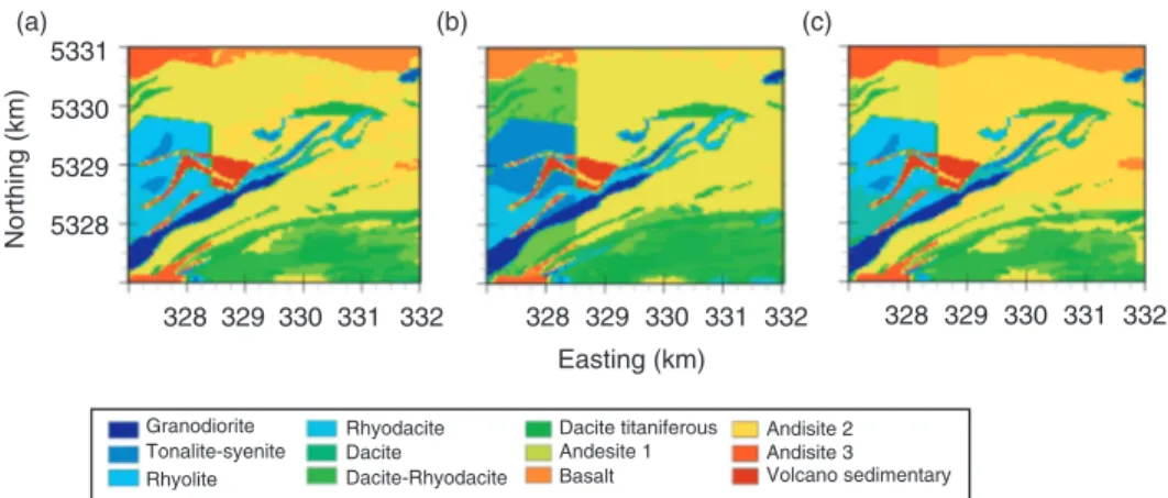
The position of the selected points, rock types, magnetization, density contrast and neurons with a constant value of 0.5 for the learning process are taken as input to the neural network. In order to simulate several rock types, magnetic susceptibility and density realizations after the training stage of the neural network, the prediction is performed by injecting an input data set and by randomly varying between 0 and 1 the neuron values of the last layer at each realization. Figures 4.a .b and .c give three selected possible realizations for the rock types. Figures 5 .a .b and .c show three possible realizations of the sub surface magnetic susceptibility. The most upper figures show horizontal maps at a depth of 930 m, at the center, vertical cross-sections down to a depth of 1600 m. Lower figures show the total magnetic field induced by the three selected realizations. The magnetic field produced by the selected models are very similar, the latter step is essential to validate the simulations, and thus for keeping the most realistic models that have similar potential field (gravity or magnetic) considered as a reference.

3.3. COMPUTER PERFORMANCES

The study area is modeled using a centered regular 3D grids (Voxet) comprising 150 ∞ 150 ∞ 75 elementary cells. The magnetic susceptibility and the density calculated from the inversion are stored at the center of each elementary cells. Ore deposits are retrieved using a regular 2D grid. The learning stage takes about 15 mn on the Intel Core 2 Duo (2.40 GHz). This is the longest step in implementing the suggested method. The prediction of a 3D cube is relatively fast, this prediction time depends on the number of simulations and the spatial resolution of the study area.

5331 5330 5329 5328 328 Northing (km) 329 330 331 332 328 329 330 331 332 328 329 330 331 332 Easting (km) Granodiorite Tonalite-syenite Rhyolite Rhyodacite Dacite Dacite titaniferous Basalt Andesite 1 Andisite 2 Andisite 3 Volcano sedimentary Dacite-Rhyodacite (a) (b) (c)

Figure 4 Horizontal cross-sections showing three possible geological maps simulated by ANN at a depth of 930 m.

4. DISCUSSION AND CONCLUSIONS

This work proposes to use a stochastic simulation method based on training neural networks. The benefits of this method are: (i) to be available to integrate several variables, (ii) it does not request a preliminary geostatistical study such as the variograms analysis to capture the spatial variability, (iii) it does not need empirical relationships between the different input and output variables. The spatial correlations are studied capture during the training stage of the neural network. These same benefits could be viewed as disadvantages as neural networks behave like black box and need a set of training images including both the sub-surface geophysical responses and a careful knowledge of the underground regarding ore deposits. Posterior analysis of the predictions allow to cross validate the results. However, other advantages of the proposed methodology are the ability of neural networks to be used not only as predictors but also as simulators. This is a very interesting tool to quantify the uncertainty related to a given exploration area. Once the neural network is completely trained, changing randomly weight neurons values of the output layer impacts the predicted results and allow generating several realizations which are conditioned by the drill holes data (considered as points). In some case, up-scaling procedure might be necessary depending on the cell sizes of the grid. Neural networks are well adapted to investigate mature brownfields in which several deposits are already been discovered at the learning stage. Assuming green fields behave like brown ones, it is then possible to apply this methodology to investigate new areas containing potential undiscovered deposits and to produce potential 3D map accounting for uncertainty.

REFERENCES

[1] A. Tarantola, “Popper, Bayes and the inverse problem,” Nature Physics, vol. 2, no. 8, pp. 492–494, 2006.

[2] A. Tarantola and B. Valette, “Generalized Nonlinear Inverse Problems Solved Using the Least Squares Criterion,” Reviews of Geophysics and Space Physics, vol. 20, pp. 219–232, May 1982.

5331 5327 328 330 332 Northing (km) Easting (km) 1.4 0 Depth (km) 5330 331 5329 Northing (km) 329 330 329 330 331 Easting (km) 58300 58200 58100 58000 57900 57800 57700 57600 57500 331 329 330 (nT) (a) (d) (e) (f) (b) (c)

[3] W. Menke, Geophysical Data Analysis: Discrete Inverse Theory. Academic Press, Inc. New York, 1984.

[4] M. Poulton, K. Sternberg, and C. Glass, “Neural network pattern recording of the subsurface EM images,” Journal of Applied Geophysics, vol. 29, pp. 21–36, 1992.

[5] E.-Q. Gad and K. Ushijima, “Inversion of DC resistivity data using neural networks,” Geophysical Prospecting, vol. 49, no. 4, pp. 417–430, 2001.

[6] C. Calderón-Macías, M. K. Sen, and P. L. Stoffa, “Artificial neural networks for parameter estimation in geophysics,” Geophysical Prospecting, vol. 48, no. 1, pp. 21–47, 2000.

[7] A. Neyamadpour, W. A. T. W. Abdullah, and S. Taib, “Use of Artificial Neural Networks to Invert 3D Electrical Resistivity Imaging Data,” AIP Conference Proceedings, vol. 1150, no. 1, pp. 210–213, 2009.

[8] G. Röth and A. Tarantola, “Neural networks and inversion of seismic data.,” Journal of Geophysical Research, vol. 99, pp. 811–822, 1994.

[9] N. Metropolis and S. Ulam, “The Monte Carlo method,” Journal of the American Statistical Association, vol. 44, pp. 335–341, 1949.

[10] J. H. Holland, Adaptation in Natural and Artificial Systems. University of Michigan Press, 1975. [11] S. Kirkpatrick, C. D. Gelatt, and M. P. Vecchi, “Optimization by Simulated Annealing,” Science,

vol. 220, pp. 671–680, May 1983. 10.1126/science.220.4598.671.

[12] C. V. Deutsch and A. G. Journel, GSLIB: Geostatistical Software Library and User’s Guide, vol. 2nd _{Edition. Oxford University Press, New York, 1998.}

[13] A. Journel and E. Isaaks, “Conditional Indicator Simulation: Application to a Saskatchewan uranium deposit,” Mathematical Geology, vol. 16, pp. 685–718, 1984. 10.1007/BF01033030. [14] T. M. Hansen, A. G. Journel, A. Tarantola, and K. Mosegaard, “Linear inverse Gaussian theory

and geostatistics,” Geophysics, vol. 71, no. 6, pp. R101–R111, 2006.

[15] M. C. Looms, T. M. Hansen, K. S. Cordua, L. Nielsen, K. H. Jensen, and A. Binley, “Geo-statistical inference using crosshole ground-penetrating radar,” Geophysics, vol. 75, no. 6, pp. J29–J41, 2010.

[16] E. Gloaguen, D. Marcotte, M. Chouteau, and H. Perroud, “Borehole radar velocity inversion using cokriging and cosimulation,” Journal of Applied Geophysics, vol. 57, no. 4, pp. 242–259, 2005.

[17] P. Shamsipour, D. Marcotte, M. Chouteau, and P. Keating, “3D stochastic inversion of gravity data using cokriging and cosimulation,” Geophysics, vol. 75, no. 1, pp. I1–I10, 2010.

[18] S. Strebelle, “Conditional Simulation of Complex Geological Structures Using Multiple-Point Statistics,” Mathematical Geology, vol. 34, pp. 1–21, 2002. 10.1023/A:1014009426274. [19] J. Caers and A. G. Journel, “Stochastic Reservoir Simulation using Neural Networks Trained on

Outcrop data,” Society of Petroleum Engineers, pp. 27–30 September, 1998. Annual Technical Conference and Exhibition.

[20] J. Caers, “Geostatistical reservoir modelling using statistical pattern recognition,” Journal of Petroleum Science and Engineering, vol. 29, pp. 177–188, 2001.

[21] T. T. Tran, “Improving variogram reproduction on dense simulation grids,” Computers and Geosciences, vol. 20, pp. 1161–1168, August 1994.

[22] P. Wong and S. Shibli, “Modelling a fluvial reservoir with multipoint statistics and principal components,” Journal of Petroleum Science and Engineering, vol. 31, pp. 157–163, 2001. [23] S. Haykin, Neural Networks A Comprehensive Foundation. Prentice Hall, New Jersey, 1999.

[24] A. Nigrin, Neural Networks for Pattern Recognition. Cambridge, MA: The MIT Press, 1993. [25] J. Zurada, Introduction To Artificial Neural Systems. Boston: PWS Publishing Company, 1992. [26] D. E. Rummelhart, G. E. Hinton, and R. Williams, “Learning internal representation by

back-propagating errors,” Nature, vol. 332, pp. 533–536, 1986.

[27] D. Singer and R. Kouda, “Application of a feedforward neural network in the search for Kuroko deposits in the Hokuroku district, Japan,” Mathematical Geology, vol. 28, pp. 1017–1023, 1996. 10.1007/BF02068587.

[28] W. M. Brown, T. D. Gedeon, D. I. Groves, and R. G. Barnes, “Artificial neural networks: a new method for mineral prospectivity mapping,” Australian Journal of Earth Sciences, vol. 47, no. 4, pp. 757–770, 2000.

[29] A. Porwal, E. J. M. Carranza, and M. Hale, “Artificial Neural Networks for Mineral-Potential Mapping: A Case Study from Aravalli Province, Western India,” Natural Resources Research, vol. 12, pp. 155–171, 2003. 10.1023/A:1025171803637.

[30] E. Werbos, The Roots of Back-Propagation. John Wiley Sons, Inc, 1994.

[31] J. R. Taylor, An Introduction to Error Analysis: The Study of Uncertainties in Physical Measurements 2nd_{Edition, University Science Books, 1997.}

[32] J. Y. F. Yam and T. W. S. Chow, “A weight initialization method for iproving training speed in feedforward neural network,” Neurocomputing, vol. 30, pp. 219–232, 2000.

[33] E. Johansson, F. Dowla, and D. Goodman, “Backpropagation Learning for Multilayer Feed-Forward Neural Networks Using the Conjugate Gradient Method,” International Journal of Neural Systems, vol. 2, no. 4, pp. 291–301, 1991.

[34] L. Wong, D. Davis, T. Krogh, and F. Robert, “U–Pb zircon and rutile chronology of Archean greenstone formation and gold mineralization in the Val d’Or region, Québec,” Earth and Planetary Science Letters, vol. 104, pp. 325–336, 1991.

[35] C. R. Scott, W. U. Mueller, and P. Pilote, “Physical volcanology, stratigraphy, and lithogeo-chemistry of an Archean volcanic arc: evolution from plume-related volcanism to arc rifting of SE Abitibi Greenstone Belt, Val d’Or, Canada,” Precambrian Research, vol. 115, pp. 223–260, 2002. [36] J. K. Mortensen, “U–Pb geochronology of the eastern Abitibi Subprovince. Part 1: Chibougamau–Matagami–Joutel region,” Canadian Journal of Earth Sciences, vol. 30, no. 1, pp. 11–28, 1993.

[37] W. Mueller and J. Mortensen, “Age constraints and characteristics of subaqueous volcanic construction, the Archean Hunter Mine Group, Abitibi greenstone belt,” Precambrian Research, vol. 115, pp. 119–152, 2002.