Dynamiques de synchronisation de lasers bifréquence à état solide et DFB soumis à une réinjection décalée en fréquence : applications en photonique micro-onde

HAL Id: tel-02062296

https://tel.archives-ouvertes.fr/tel-02062296

HAL is a multi-disciplinary open access archive for the deposit and dissemination of sci-entific research documents, whether they are pub-lished or not. The documents may come from teaching and research institutions in France or abroad, or from public or private research centers.

L’archive ouverte pluridisciplinaire HAL, est destinée au dépôt et à la diffusion de documents scientifiques de niveau recherche, publiés ou non, émanant des établissements d’enseignement et de recherche français ou étrangers, des laboratoires publics ou privés.

état solide et DFB soumis à une réinjection décalée en

fréquence : applications en photonique micro-onde

Aurélien Thorette

To cite this version:

Aurélien Thorette. Dynamiques de synchronisation de lasers bifréquence à état solide et DFB soumis à une réinjection décalée en fréquence : applications en photonique micro-onde. Optics / Photonic. Université Rennes 1, 2018. English. �NNT : 2018REN1S059�. �tel-02062296�

T

HESE DE DOCTORAT DE

L'UNIVERSITE DE RENNES 1

C

U

B

L

Matière, Molécules, Matériaux

Spécialité : « Physique »

Synchronization dynamics

of dual-mode solid-state and semiconductor DFB lasers

under frequency-shifted feedback.

Applications to microwave photonics.

Unité de recherche : Institut FOTON / DOP

Par

Aurélien THORETTE

Professeur, ENSICAEN

Maître de conférences, Université de Montpellier 2 Professeur, Telecom ParisTech

Maître de conférences, Université de Nice-Sophia Antipolis Ingénieur, III-V Lab Palaiseau

Professeur, Université de Rennes 1

Maître de conférences, Université de Rennes 1 Hervé GILLES, président

Stéphane BLIN, rapporteur Frédéric GRILLOT, rapporteur Giovanna TISSONI, examinatrice Frédéric VAN DIJK, invité

Marc VALLET, co-directeur de thèse Marco ROMANELLI, co-directeur de thèse

Thèse soutenue à Rennes le 30 novembre 2018

devant le jury composé de :

3

R

EMERCIEMENTS

L

trois années de thèse doit beaucoup à la présence constante et aux échanges scientifiques quotidiens que j’ai pu avoir avec mes directeurs, Marco Romanelli et Marc Vallet (ex-æquo). Je me suis rendu compte au fil des rencontres avec d’autres thésards de tous horizons qu’il est finalement bien rare de bénéficier d’un encadrement d’un tel acabit.

Entre les lignes de cette thèse, il faut aussi voir la compétence de très haut niveau, et plus généralement la patience et la pédagogie des électroniciens Ludovic Frein et Steve Bouhier, et de l’ingénieur ès fibres optiques, Goulc’hen Loas. J’y associe également Anthony Carré pour la partie optique et informatique, et Cyril Hamel pour la mécanique. Marc Brunel mérite une mention particulière, pour avoir gardé une attention sur ces travaux, et pour sa disponibilité à discuter des problèmes rencontrés. Une partie du matériel utilisé est issu du projet EDA HIPPOMOS, dont je remercie les différents partenaires pour les composants uniques dont j’ai pu bénéficier. Sur ce volet, je me contenterais de mentionner que les efforts de Mehdi Alouini y sont pour beaucoup.

Marie Guionie a droit à sa propre phrase complète, au titre de collègue de bureau presque agréable, stagiaire M2 efficace, et grande cheffe de Pint of Science à Rennes, qui fut une belle expérience. J’en profite pour en saluer les autres participants.

Dans le désordre, salutations amicales aux collègues du DOP : Julien, François P. Romain, François B., John, Kévin, Gwennaël, Gaëlle, Hongzhi, ainsi qu’à ceux que je n’ai que brièvement croisés et que j’oublie peut-être : Swapnesh, Nolwenn, Céline, Noé, Tron, Esteban, Tore, Ayman, Emmanuel, ...

Cette thèse s’est achevée à l’Institut FOTON et a débuté au sein de l’Institut de Physique de Rennes (IPR). J’adresse donc une salutation globale aux collègues des deux instituts, notamment aux personnels administratifs, et aux chercheurs que j’ai pu rencontrer lors de mon expérience d’enseignement. J’adresse un remerciement plus particulier à Guillaume Raffy, Alexandra Viel et Jérémy Gardais de l’équipe SIMPA, pour m’avoir prêté jusqu’au bout du temps de calcul, et apporté le soutien technique associé.

Enfin, je remercie Fréderic Grillot et Stéphane Blin d’avoir accepté de rapporter ces travaux, Hervé Gilles d’avoir bien voulu présider le jury, Giovanna Tissoni en qualité d’examinatrice, et Frédéric Van Dijk pour sa présence lors de la soutenance.

5

R

ÉSUMÉ DES RÉSULTATS

C

syn-chronisation en phase de deux lasers. Plus précisément, est étudiée une méthode appelée réinjection décalée en fréquence, qui vise à obtenir le verrouillage sur une référence de la différence de fréquence entre deux lasers. En pratique, cette différence de fréquence se situant dans le domaine micro-onde, ces travaux sont à l’intersection de la dynamique des lasers et de la photonique micro-onde.

LE PREMIER CHAPITREest introductif et vise à rappeler les principes fondamentaux

et les équations de base régissant la dynamique de lasers de classe B. Une dérivation des “rate equations” standards est proposée. Une partie est consacrée plus précisé-ment au facteur de Henry (α), en raison de sa grande influence lors de l’étude de dynamiques sous injection. Sa définition est rappelée, et est poursuivie par une brève revue des différentes méthodes permettant de le mesurer. Disposant de ces éléments, quelques résultats élémentaires sont rappelés pour le cas d’un laser injecté, et d’un laser soumis à une rétroaction (feedback). Les concepts de bifurcations, de plage d’accrochage, de modes de cavité externe sont présentés. La suite du chapitre permet de présenter le contexte de la photonique micro-onde, et notamment la technique de génération hétérodyne, c’est-à-dire utilisant le battement entre deux fréquences optiques comme source de fréquence dans le domaine micro-onde. Les avantages de cette approche et les difficultés rencontrées sont énumérés, en aboutissant au besoin d’une stabilisation supplémentaire du battement. Une revue des techniques existantes est présentée, en insistant particulièrement sur le fort intérêt qu’il y a à générer les deux fréquences optiques dans un unique laser. Une option, le laser bipolarisation bifréquence, utilise la levée de dégénérescence des modes de polarisation d’une cavité laser pour générer deux modes orthogonaux de fréquences différentes. Les résultats existants sur ce type de configuration sont rappelés.

LE SECOND CHAPITRE porte sur l’application de la méthode de stabilisation par

réinjection décalée en fréquence à un laser bipolarisation à état solide Nd:YAG. Il s’agit de réaliser une injection optique d’un mode de polarisation du laser sur l’autre. Or, une injection résonante n’est possible que pour un faible désaccord de fréquence entre le champ injecteur et celui de la cavité. Une étape de décalage en fréquence, utilisant ici un modulateur acousto-optique est donc utilisée. De plus, la séparation en polarisation des deux modes permet une injection unidirectionnelle.

verrouillage de phase entre les modes est observé. Il correspond à un report complet de la stabilité de la référence (ici, le signal de décalage) sur le battement laser. Un modèle basé sur des rates equations est présenté, incluant les termes d’injection et de saturation croisée liés au fonctionnement bipolarisation. Ce modèle, sous une forme normalisée, est à la base de l’étude numérique. L’étude des bifurcations de l’état stationnaire permet en effet d’identifier, outre la zone d’accrochage de phase, une zone de verrouillage partiel. Dans cette région, un régime de phase bornée est observé numériquement et expérimentalement. Il correspond à un verrouillage de la fréquence moyenne, malgré des oscillations d’amplitude et de phase. Une étude numérique plus exhaustive est menée pour les cas de faible injection, pour lesquels de nombreux régimes chaotiques existent. On peut ainsi mettre en évidence un régime particulier, combinant des propriétés de phase bornée et des fluctuations chaotiques. Ce régime dit de chaos borné est également observé expérimentalement. L’étude du bruit de phase montre qu’il s’agit toujours d’un régime de synchronisation moyenne forte.

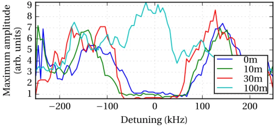
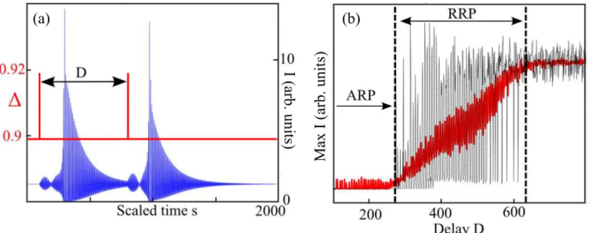
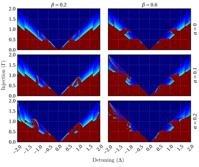
D’autres études sont menées autour de ces zones de faible injection. Première-ment, un retard est ajouté dans le bras de réinjection sous la forme d’une bobine de fibre. On montre que pour des retards correspondant à quelques périodes des oscillations de relaxation, une réduction de la plage d’accrochage est observée, ainsi qu’une dégradation du bruit de phase. D’autre part, un mécanisme de type excitabilité est mis en évidence sur les bords de la plage d’accrochage. On peut en particulier conserver le caractère borné de la phase pendant le déclenchement d’un événement. Enfin, les études précédentes ont été reproduites pour plusieurs valeurs du coefficient de saturation croisée β et du facteur de Henry α.

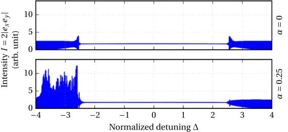
Ce dernier facteur, rarement pris en compte dans les lasers à état solide, a en effet été ajouté dans le modèle pour rendre compte d’observations expérimentales. Les asymétries observées sur la plage d’accrochage, et notamment la différence de type de décrochage observé en fonction du signe du désaccord, sont en effet un marqueur typique d’un facteur α non nul. Une méthode de mesure ad-hoc de ce coefficient a été développée, en tirant partie d’une légère modification du dispositif expérimental. L’introduction d’une perturbation de phase par injection optique se reporte sur l’intensité de sortie via le couplage phase-amplitude lié à α. Or, il existe une valeur critique du désaccord pour laquelle ce n’est pas le cas. La mesure de celle-ci permet de remonter à α. La mise en œuvre de cette méthode «FM/AM» se réduit dans notre cas à introduire une modulation de fréquence sur le signal de référence. À l’aide du modèle, on obtient ainsi une mesure précise et originale α = 0.28 ± 0.04.

Finalement, cette méthode de stabilisation par réinjection décalée en fréquence a aussi été appliquée à un autre type de laser bipolarisation, un laser fibré de type

7

DFB. Dans ce début d’étude, nous avons constaté que le verrouillage est possible et robuste, mais que le facteur de Henry probablement plus élevé mène à des formes plus complexes de la plage d’accrochage.

LE CHAPITRE III est consacré à la transposition de cette méthode de réinjection

décalée en fréquence à un système plus proche des applications potentielles. Il s’agit cette fois de deux lasers semi-conducteurs distincts, de type DFB, situés sur une même puce. Ces composants originaux sont développés et produits par le III-V Lab, en tant que générateurs hétérodyne pour des applications télécom, radar, etc. Dans cette optique, ils présentent une faible largeur de raie, autour de 300 kHz ainsi qu’une large bande passante de modulation. Leur accordabilité est large, et dans notre cas, nous utilisons un battement de 10 GHz entre les deux lasers.

Afin de verrouiller en phase ces deux lasers, une boucle fibrée de réinjection décalée en fréquence est réalisée, incluant un modulateur d’intensité. L’utilisation de ce dernier, motivée par les hautes fréquences à atteindre, a pour conséquence un mécanisme de couplage plus complexe que précédemment entre les deux lasers. En effet, chaque laser est injecté optiquement par l’autre laser, mais il subit aussi son propre feedback. De plus, ces lasers ayant des temps caractéristiques rapides (de l’ordre de la nanoseconde), le temps de parcours dans la boucle de feedback ne peut être négligé, ce qui nous met en présence de dynamiques à retard long. Néanmoins, nous montrons expérimentalement, mais aussi numériquement que le verrouillage de phase est possible. Un modèle numérique basé de type “rate equations” a en effet été développé pour décrire le couplage retardé entre les lasers. À cette fin, une bonne connaissance des paramètres du système est nécessaire. Ainsi une caractérisation poussée des lasers a-t-elle été réalisée, notamment les différents temps de vie (obtenus par l’intermédiaire d’une mesure de la fonction de transfert en modulation) et le facteur de Henry (obtenu par une méthode d’injection optique statique).

Outre le régime de verrouillage de phase, qui permet, comme dans le cas du laser bipolarisation, de transférer la pureté spectrale de la référence vers le battement, des régimes de synchronisation partielle sont observés expérimentalement et numérique-ment. À la différence du cas bipolarisation, on observe un morcellement de la zone de stabilité en fonction du désaccord, qui forme des « bandes d’accrochage ». La périodicité de ces bandes est reliée à la fréquence de la cavité externe, c’est-à-dire au retard. Cette alternance de zone de verrouillage, avec des zones de décrochage ou de synchronisation partielle, type phase bornée, a pu être observée très nettement que ce soit expérimentalement et numériquement.

Parmi les nombreux paramètres présents dans ce système, les phases optiques liées à chaque terme de couplage ont fait l’objet d’une attention particulière. En effet, ces paramètres sont mal contrôlés expérimentalement, et peuvent être sujets à de fortes

dérives. Or leur valeur peut changer de façon importante l’état stationnaire atteint par le système. C’est pourquoi nous avons étudié numériquement l’influence de ces phases optiques sur l’état final du système, et ce en fonction des différents taux de couplage, ainsi que pour différents retard. Il apparaît qu’il est possible de minimiser l’influence de ces paramètres sur le régime verrouillé en privilégiant l’injection croisée entre les lasers et en minimisant le feedback pour chacun d’entre eux. D’autre part, il semble que la présence d’un retard long permette également de diminuer l’influence de ces phases.

DANS LE CHAPITREIV, le système précédent est réutilisé, mais dans une

configu-ration « boucle fermée », c’est-à-dire en s’affranchissant de la référence externe. Un retard, sous la forme d’une bobine de fibre, est utilisé pour verrouiller le battement sur lui-même. En ajoutant un filtre passe-bande électrique dans cette boucle résonante, on obtient une configuration assez similaire ce qui est couramment connu sous le nom d’oscillateur opto-électronique (OEO). À la différence de ces montages, qui se basent habituellement sur un modulateur d’intensité, notre signal de sortie contient uniquement les deux fréquences optiques associées à chaque laser. Cette propriété, dite de bande latérale unique, rend le taux de modulation du signal insensible à la dispersion chromatique, et donc approprié à la transmission dans une longue liaison fibrée.

Ce montage expérimental, réalisé sans grande isolation de l’environnement, per-met d’obtenir de bonnes performance de bruit de phase, jusqu’à −95 dBc/Hz à 10 kHz de la porteuse à 10 GHz. Le bruit de phase présente les caractéristiques typiques d’un OEO : décroissance en basse fréquence relative, puis pics de résonances liés au retard utilisé. Ces derniers peuvent être réduits en utilisant des techniques issues des développements sur les OEO. Par exemple, nous avons montré l’efficacité d’un schéma basé sur deux retards différents formant un interféromètre dans le domaine micro-onde.

Finalement, la présence d’une longue cavité externe dans le système de réinjection décalée en fréquence impose l’usage d’un filtre RF sur-mesure, avec une bande passante particulièrement faible. Cette contrainte peut être levée en réduisant la cavité externe. Nous avons développé un système beaucoup plus compact, qui utilise une simple réflexion comme cavité externe, et une faible modulation directe du courant de pompe d’un des lasers comme mécanisme de décalage en fréquence. On peut dès lors utiliser un filtre RF beaucoup plus standard, et obtenir, avec un montage très simple, un signal optique micro-onde quasiment à bande latérale unique.

Dès lors, de nombreuses perspectives apparaissent, comme l’intégration du mod-ulateur, voire du retard sur le composant, chose qui a déjà été réalisée au III-V Lab. Enfin, l’utilisation du modèle développé au chapitre III peut permettre de réaliser une

9

analyse plus quantitative du système pour guider son amélioration.

EN CONCLUSION, cette étude de la réinjection décalée en fréquence dans deux

cas différents permet de mettre en avant les propriétés globales de cette méthode de couplage entre deux lasers, ou deux modes du même laser. L’influence d’un grand nombre de paramètres a été étudiée, que ce soit pour le régime de verrouillage, ou pour des régimes de synchronisation partielle. La combinaison d’études expérimen-tales et numériques a permis de garder une perspective résolument tournée vers les applications et la caractérisation des performances, sans pour autant négliger l’étude de la dynamique et des régimes instables. La versatilité de cette technique et la bonne compréhension de son fonctionnement amène finalement à envisager des développements futurs pour d’autres types de lasers, que ce soit dans des milieux actifs différents (Erbium, fibre, semiconducteurs multifonctionnalités) ou encore pour des fonctionnements multimodes.

11

T

ABLE OF CONTENTS

Table of symbols 15

General introduction 17

I Introduction to injection and feedback in lasers, and to microwave photonics 21

1 Dynamical modeling of class-B lasers . . . 21

1a The laser rate equations . . . 21

Evolution of the field . . . 22

Population inversion . . . 25

Rate equations and their properties . . . 26

1b The linewidth enhancement factor α . . . 29

Definition, consequences and typical values . . . 29

How to measure it? . . . 30

2 Interaction dynamics and their usages . . . 32

2a Injection and synchronization . . . 32

The Adler equation . . . 33

Beyond the Adler equation . . . 34

2b Feedback in lasers . . . 36

Lang-Kobayashi equation and external cavity modes . . 37

3 Microwave photonics . . . 39

3a Characteristics of a microwave signal . . . 40

3b Dual-frequency lasers . . . 42

Heterodyne microwave generation. . . 42

Dual-polarization lasers . . . 43

4 Conclusions. . . 46

II Frequency-shifted feedback in dual-frequency solid state lasers 47 1 Dual-frequency dual-polarization laser . . . 47

Frequency separation . . . 48

Pump diode . . . 49

2 Frequency difference locking using feedback . . . 50

2a Experimental setup. . . 51

2b Rate equations model . . . 52

Analytical study . . . 54

3 Results . . . 58

3a Locked state, bounded phase . . . 58

Steady state and bifurcation diagram . . . 58

Bounded phase oscillations . . . 60

3b Exhaustive mapping for Γ.1. . . 61

4 Bounded phase chaos . . . 65

Numerical prediction. . . 65

Experimental observation . . . 66

Phase noise properties . . . 67

4a Influence of the feedback delay. . . 69

4b Bounded chaotic “spike triggering” (excitable-like) . . . 73

4c Arguments in favor of a non-zero α . . . 77

4d Alternate results for α = 0 and β = 0.6 . . . 79

5 Application to the measurement of the small linewidth enhancement factor. . . 82

5a Theory . . . 82

5b Dual-frequency laser . . . 84

5c Result for Nd:YAG bulk laser . . . 87

6 Fiber laser . . . 89

7 Conclusions. . . 94

III Synchronization and complex dynamics of two coupled semiconductor lasers 95 1 The dual-DFB component . . . 95

1a Tunability . . . 98 1b Frequency stability . . . 99 1c Linewidth . . . 100 1d Lifetimes measurements . . . 102 Principle . . . 102 Results . . . 104

1e Linewidth enhancement factor . . . 104

Principle . . . 105

Experimental realization. . . 107

Results . . . 108

2 Setup and model for frequency-shifted feedback . . . 110

2a Experimental setup. . . 110

2b Delayed rate equations . . . 111

Resonant approximation and the relevant terms. . . 111

Rate equations and normalization . . . 112

Injection rates . . . 114

Summary of the parameters . . . 115

Estimating the drift of the feedback phases . . . 116

13

2d Injection rate estimation . . . 118

2e Modulation ratio . . . 120

3 Comparison of numerical and experimental results . . . 120

3a Observed regimes. . . 121

Experiments . . . 121

Simulations . . . 122

“Full” model simulations . . . 123

3b Multistability . . . 124

3c Phase dependency . . . 125

3d Influence of frequency detuning: locking range . . . 127

3e Locking bands. . . 129

3f Overall stability and phase noise . . . 130

4 Conclusions. . . 132

IV Hybrid opto-electronic oscillator 135 1 The opto-electronic oscillator . . . 135

1a Principle . . . 135

1b Phase noise . . . 137

1c Dispersion losses in long fiber links . . . 138

2 Long-delay setup. . . 139

2a Setup . . . 140

2b Performances and challenges. . . 141

2c Dual-loop . . . 143

3 Shorter delays, towards integration . . . 145

3a Straight feedback and direct modulation . . . 145

4 Transfer functions: towards a full model of the hybrid OEO. . . 149

4a On-chip feedback . . . 151

5 Perspectives. . . 153

Conclusions and perspectives 155 Annexes 159 A Eigenstates of a cavity with two quarter-wave plates . . . 159

B Estimation of α from gain asymmetry . . . 162

C Coupling factor β for an non-isotropic pumping . . . 165

D Comparison of integrators for phase noise calculation . . . 169

E A Python wrapper for the DDE integrator RADAR5 . . . 171

Associated publications 173

15

T

ABLE OF SYMBOLS

Through this work, for a variable x, bx denotes the associated steady-state value. The symbol i is used for the imaginary unit without exception, while j is used for indexing. The following global notations are used in different places through the document. The more local notations, used a few times in a single section, are not included in this table.

c Speed of light in the vacuum.

E Complex amplitude of the slowly-varying electric field. Einj Complex amplitude of the injected field.

Ej Complex electric field.

f0 Reference microwave frequency.

fAO Driving frequency for the acousto-optic modulator.

fM Frequency modulation frequency.

f_R(j ) Relaxation oscillations frequency (possibly of laser j ).

g Normalized laser gain. G Amplifier gain.

I Optical intensity (Chapter I) or power (Chapters II to IV).

I,_Q In-phase and quadrature components of a demodulated signal.

K Feedback or injection strength. ` Cavity length.

L Phase noise (in dBc/Hz).

L Feedback length (Chapter II and III). Fiber coil length (Chapter IV). m Modulation ratio associated to the Mach-Zehnder modulator.

n Optical index of the active medium (Chapter I), or of the fiber (Chapter II to IV). N Difference of population inversion density from the threshold level.

N Population inversion density.

Nth Population inversion density at laser threshold.

P Pump term. In the case of semiconductor lasers, pump current.

P Electric polarization of the active medium.

r Pumping ratio. Rp Pumping rate.

Rp,th Pumping rate at laser threshold.

s Normalized time, related to the relaxation oscillations pulsation. Sϕ Phase noise (in dBrad2/Hz).

t0 Field transmission coefficient for the modulator.

t1,2,C Field transmission of the output coupler for each laser, or for one of them.

T Feedback delay.

X Demodulated beatnote amplitude. α Linewidth enhancement factor.

β Cross-saturation coefficient.

Γ Normalized injection rate. ∆,δ Normalized frequency detuning.

∆0 Mean detuning (Chapter II). Half-width of locking range (Chapter III) ∆m Mean detuning of minimal amplitude response (Chapter II).

Detuning of unchanged intensity output (Chapter III).

δν Frequency detuning.

∆+,− Normalized locking range boundaries.

ε Damping coefficient.

η Effective pumping ratio.

θ Angle of a quarter-wave plate, either in the cavity or for the pump (Chapter I). Phase difference between the two lasers (Chapter III).

κ Normalized feedback strength. λ Laser wavelength.

νx,y,1,2 Optical frequency of mode x/y, or of laser 1/2.

τ Normalized feedback delay (Chapters I, II and III). Opto-electronic delay,

unnor-malized (Chapter IV).

τc Carrier lifetime (even for solid-state lasers), related to the decay of population inversion.

τp Photon lifetime, related to cavity losses.

χ,χr,χi Electric susceptibility of the active medium, and its real and imaginary part respectively.

ϕ Phase of the electric field under injection (Chapter I). Phase difference between the two modes (Chapter II).

ϕ1,2,x Optical feedback phases (Chapter III).

φ Output phase of the microwave signal (Chapter IV). ψ Phase of the injected field.

ω Pulsation of the monochromatic field under study.

ω0 Resonant optical pulsation of the cavity.

17

G

ENERAL INTRODUCTION

T

theoretical advances. While the theoretical background was already there, most notably due to Einstein [Einstein17], the experimental breakthrough came from first realization of microwave-domain masers by Gordon, Zeiger and Townes [Gordon55]. The latter, along with Schawlow, then predicted that a similar device, but operating in the visible spectrum could be made [Schawlow58]. The same suggestions were made by Basov and Prokhorov [Prokhorov58], and it was not long since the first laser was indeed realized by Maiman using a crystal of ruby [Maiman60]. At that time, the booming of researches on semiconductors and the premises of the associated industry quickly allowed the fabrication of semiconductor-based lasers [Basov61;

Hall62;Nathan62]. Ever since then, they have become ubiquitous, and an integral part of many consumer systems or research equipment.

While lasers have completely revolutionized optics, they also made their way into almost every field of science and technology. To illustrate this, we will cite only two very different examples. First, we cannot but admire the success of fiber-optics communication networks, which use laser diodes as transmitters, and allow for ever-rising transfer speed and volumes [Agrawal02]. Second, the recent detection of gravitational wave signals with the LIGO and VIRGO detectors [Abbott16] has been made possible also thanks to the ultrastable solid-state lasers at the core of the giant interferometers [Bondu96;Acernese09].

While these two examples seem quite remote from each other, they were chosen to illustrate the vast area in which this thesis takes places, namely the stabilization of lasers, or even more generically the dynamics of lasers. Indeed, the evolution of telecommunication systems or the increasingly finer metrology experiments require even more stable lasers, or lasers with particular behaviors.

This very wide problem has attracted a lot of attention and generated countless developments. Putting aside pulsed regimes such as mode-locked lasers, for which considerable efforts have been made [Udem02], and focusing only on continuous-wave lasers, many solutions have been proposed and successfully applied. For

inten-sity stabilization, the most common are based on “noise-eating” electronic feedback loops, which use a measurement on the laser’s output and a counter-reaction on one of its parameter, such as pump or temperature. For frequency stabilization, it is common to use the interaction with a frequency etalon, such as the absorption by a molecular transition in a gas cell, or the reflection from a Fabry-Perot cavity. The most prominent example of this is the Pound-Drever-Hall method and its variations [Drever83]. A different scheme uses the optical locking of the laser on an external cavity, such as a Fabry-Perot resonator [Salomon88] or a long fiber [Kéfélian09]. This is usually obtained by allowing a certain level of feedback from the external resonator into the laser.

In this work, we will focus on a subset of laser stability problem: rather than the absolute stabilization of a laser, we will study a method that allows to stabilize the frequency difference between two lasers. This frequency difference corresponds to a beatnote usually falling in the microwave domain. Thus, our work falls at the intersection between optics and the high-frequency electronics needed to process these beatnotes. This quite new domain called microwave photonics, arises partly from the fact that large microwave frequencies, i.e. over 10 GHz, are sometimes much easier to handle, generate, transport or process when placed on an optical carrier, rather than on a coaxial cable [Yao09].

Among the most obvious problems addressed by microwave photonics are the “radio-over-fiber” cases, for instance in high-speed telecommunications, or antenna remoting for wireless systems such as radar [Xu14] or radioastronomy [ Montebug-noli05].

The generation of microwave signals can also benefit from interactions with optics. Indeed, it is well known that the higher the frequency, the harder it is to generate it with conventional methods. This applies in terms of complexity, cost, and output signal quality [Rohde14]. For all these points, the use of optical beatnotes shines as an attractive alternative. Indeed, such heterodyne methods are conceptually simple and inherently widely tunable with few frequency-dependent noise.

To illustrate this, one of the main interests of such heterodyne methods is that very high frequencies, often barely reachable with all-electronic techniques can be obtained [Rolland14]. For instance, fast progresses in the the field of terahertz waves [Tonouchi07] and their potential applications in biology [Pickwell06], de-fense [Davies08], chemistry [Mouret13] or wireless communications [Federici10] drive the search for tunable and high-quality sources.

However, heterodyne methods suffer from the fact the fluctuations of each laser’s wavelength and amplitude are reported on the beatnote. Thus, stabilization tech-niques have to be applied, and no standard, widely usable method has arisen yet.

19

Methods derived from the stabilization of a single laser can be used, by applying them on the two sources [Day92; Hallal16]. Otherwise, sole stabilization of the beatnote can be obtained using similar methods, based on feedback loops and locking on an external reference [Alouini01;Rolland11b].

The optical frequencies involved in the generation of the beatnote can be obtained from either two different lasers, or from multiple modes of a laser. For instance, optical frequency combs are commonly used [Fortier11]. In our lab, we develop and propose another approach: we generate the two frequencies from a single laser, that functions on its two orthogonal polarization axes. Such polarization

dual-frequency lasers [Bretenaker90] have interesting properties in terms of tunability and free-running stability, that led to some achievements in terms of THz beatnote gen-eration [Alouini98;Brunel04;Danion14] and optically-carried high-purity microwave signals [Pillet08]. Stabilization techniques have been developed for these lasers, with extensions towards very high frequency beatnotes [Rolland11a]. More details on the properties of dual-polarization lasers, along with a quantitative description of some realizations will be given inChapter I.3b.

We see here that a lot of stabilization techniques are based on a mechanism of con-trolled optical feedback or injection. However, in the history of the laser, injection and feedback have not always been seen as stabilizing features. On the contrary, feedback is often seen as destabilizing [Henry86], and so can be an external injection [Tredicce85]. The experimental observations, combined with numerical models of such phenomena form the raw material of a field known as laser dynamics. The viewpoint here is to consider lasers under different couplings as dynamical systems. How they react under variations of their parameters is studied, and a wide range of effects are found, from self-sustained oscillations, to chaotic behavior, or synchronization mechanisms between multiple lasers [Erneux10;Sciamanna15].

In this thesis, we will study in more depth an injection-based method called

frequency-shifted feedback (FSF). This technique is based on the resonant injection

from one laser into the other, and allows to synchronize their phase. In turn, the difference between the frequencies of the two lasers produces a much more stable beatnote. It was originally proposed a few years ago [Kervevan07], and has shown promising results when applied to the two modes of a dual-frequency solid-state laser [Thévenin12c]. Here, we will continue this study, and also try to adapt the technique to separate semiconductor lasers. All this will be done from a twofold point of view: first, the applicative microwave photonics viewpoint of beatnote stabilization, and second also the more fundamental framework of the study of coupled laser dynamics.

Outline

This manuscript is structured in four chapters. Thefirst onewill be devoted to a short and simplified recall of the rate equations theory, and how they can be used to describe the dynamics of a class-B laser. Namely, they can be successfully applied to the case of lasers subjected to the optical injection from another laser, or to feedback from themselves. The microwave photonics framework of this work will be also presented, and specifically the heterodyne generation of microwave signals. With respect to that challenge, we will see that dual-polarization dual-frequency lasers are particularly fit for the task but require stabilization mechanisms.

In the second chapter, we will focus on a form of stabilization using frequency-shifted feedback, applied to a solid-state dual-frequency dual-polarization Nd:YAG laser. Building on previous results from our lab, we will show experimentally and numerically that depending on a number of parameters, different types of synchro-nization regime between the two polarization modes can be obtained. We will also measure the value of the often ignored linewidth enhancement factor, and highlight its influence in the reinjection dynamics.

Chapter III will be devoted to another type of beatnote-generating device. This time, two separate semiconductor lasers provided by III-V Lab will be used, with the particularity of being located on a single semiconductor component. We will see that FSF can still be applied, but that more complex phenomena take place, namely because of the higher number of couplings between the lasers, and the fact they are ruled by delayed dynamics. Nevertheless, thanks to a careful characterization of the components, we will develop a numerical model and see that its results compare well with experimental observations.

Theses results will be used in Chapter IVin order to build a proof-of-concept of a self-referenced heterodyne oscillator. By combining FSF and the concept of the opto-electronic oscillator (OEO), we will show that microwave signals over optical carriers can be obtained with good phase noise performances. Perspectives, among which integration on photonic components and precise model-driven design will be discussed.

A shortconclusive sectionwill summarize the different achievements, and discuss the horizon of perspectives, suggesting future work to be done.

21

C

HAPTER

I

I

NTRODUCTION TO INJECTION AND

FEEDBACK IN LASERS

,

AND TO MICROWAVE

PHOTONICS

1

Dynamical modeling of class-B lasers

In this thesis, one of our task will involve modeling of lasers. Thus, in this first part, we will recall some standard concepts, results and make a brief derivation of the tools that will be extensively used afterwards.

1a

The laser rate equations

T

the acronym LASER, namely “Light Amplification by Stimulated Emission of Radiation”. Indeed, it is based on a light-matter interaction process called stimulated emission, where the deexcitation of elements in an active medium allows to coherently amplify a light field. This process can be summarized as the effective duplication of an incident photon, accomplished during this deexcitation. The energy of the supplementary photon corresponds to the difference between the upper, excited level and the lower level after the transition. This is sketched on Fig. I.1. While the principle is the same for all lasers, widely different active media exist, from gas molecules, ions trapped in crystalline, glass matrices or fibers, to semiconductor lasers where laser emission relies on electron-hole recombination. Alongside, the process of pre-excitation of the active medium, called pumping, can differ a lot, and can be provided for instance by another light source, an electric spark, or an electric current [Verdeyen95; Svelto10]. Having realized a “light amplifier”, it is placed in an optical cavity, schematically two face-to-face mirrors, so that each photon makes

multiple round-trips, and has multiple chance to trigger stimulated emission. When the gain of the amplification compensates the losses in the cavity or at its ends, the

laser threshold is reached, and the laser phenomenon begins.

ν

ν

Nd

_{excited state}

Nd

_{ground state}

ν

conduction band

(electrons)

(holes)

valence band

Figure I.1: Principle of stimulated emission amplification, in a four-level solid state medium, such as Nd:YAG (left) and in a semiconductor (right).

The fact that some elements of the active medium are being pumped into an excited level comes unavoidably with the fact that they may randomly decay into a state of lower energy. By doing so, they will generate non-coherent light, composed of photons with random direction, polarization and wavelength. This phenomenon, called spontaneous emission, is one of the main sources of noise in lasers. However, in all the following, we will not be interested in the intrinsic noise of our lasers, so this phenomenon will be neglected in all our models. This approximation is justified for solid-state lasers, which have a low level of spontaneous emission above threshold [Koechner06]. This is not the case in many types of semiconductor lasers, but we will only be interested in models that have a sufficiently low noise levels, and used way above threshold, so that spontaneous emission can be neglected.

Evolution of the field

First modeling of the laser phenomenon was done almost as soon as the first ob-servation of the effect, and was built upon the previous model of the MASER, the microwave domain predecessor of the laser [Schawlow58; Lamb64]. Afterwards, numerous approaches to describe the laser phenomenon have been developed with varying complexity. A semi-classical treatment uses the density matrix formalism and leads to the Maxwell-Bloch equations, that may also be designated as Arecchi-Bonifaccio equations after their discoverers [Arecchi65;McNeil15]. Other approaches, either generic or more specifically applied to certain types of lasers, are also common and lead to similar results in the usual cases [Agrawal86; Tartwijk95; Petermann88;

1. DYNAMICAL MODELING OF CLASS-B LASERS 23

schematically this form:

field_{E −→} 1

acts onions, atoms, electrons, etc. 2 −→ generatepolarizationP 3 −→ drivesfieldE Here the electric field in the cavity_E interacts with the active medium (step 1 ). The interaction process can be rather complex, and its accurate description is often only possible using a quantum mechanics point of view. However, ultimately, it will lead to an electric polarization _P of the medium (step 2 ) so that it is possible to phenomenologically account for this response. Conversely, the response can be simply experimentally measured. Finally, this electric polarization acts as a driving force for the electric field (step 3 ), and the loop is repeated again [Sargent74]. We will present here a simplified derivation of the laser equations, based on this principle.

Wave equation. We will assume that the laser cavity selects an axis z, and will neglect any transverse aspect of the field. Also, the model will be scalar, and will not take polarization effect into account, although this can be done in extensive models [Chartier00]. We will not make any assumption on the shape of the active medium, or on whether it occupies the whole cavity or not. Starting from the Maxwell equations, and with all these assumptions, we can write the following wave equation for the time evolution of the cavity field_E along the cavity axis z:

∂2_E ∂z2− n2 c2 ∂2_E ∂t2− n2 c2_τ p ∂_E ∂t = µ0 ∂2_P ∂t2 (I.1)

There, c is the speed of light in vacuum, n is the index in the cavity. Here we consider a non-magnetic medium, so that µ0 is the vacuum magnetic permittivity. We have introduced phenomenologically a decay term with time scale τp, that cor-responds to the distributed losses along the cavity, including what is due to output mirrors, optical elements, conductivity of the medium, etc. This quantity is often called the “photon lifetime”. Finally, the right-hand side is a driving term, that corresponds to the interaction of the field with the gain medium. This produces an electric polarizationP, which in turn drives the evolution of the field.

We consider a monochromatic field with an arbitrary pulsation ω, _E(z, t) =

E(t)ei ωt−ikz_{+ c.c., and are only interested in its complex amplitude E(t). Here k is} the wavenumber corresponding to the resonant mode of the cavity, so that k = nω0/c where ω0 is the resonant pulsation. We note here a first approximation, that is that the intensity |E|2 _{of the field does not vary appreciably along the cavity. This is} obviously true for cavities with good mirrors, but may not be correct for some long

semiconductor lasers. However, we will only be interested in distributed feedback semiconductors (DFB), which have low photon lifetimes. This gives the following time and space derivatives:

∂_E ∂t = µ_dE dt + iωE ¶ ei ωt−ikz_{+ c.c.} (I.2a) ∂2_E ∂t2 = µ 2i ωdE dt − ω 2_{E +}d2E dt2 ¶ ei ωt−ikz_{+ c.c.} (I.2b) n2c2∂ 2_E

∂z2 = −n2c2k2Eei ωt−ikz+ c.c. = −ω20Eei ωt−ikz+ c.c. (I.2c) We suppose that the rotating frame pulsation ω is close to the resonant frequency

ω0, so that ω2−ω20

ω ≈ 2(ω−ω0). This will add a frequency detuning term in the final wave equation.

Slowly Varying Envelope Approximation (SVEA). As we suppose that the complex amplitude E varies slowly compared to the optical frequencies, we can remove most terms of the previous derivatives using what is often called the slowly variable envelope approximation (sometimes abridged as SVEA), which is applicable when¯¯dE

dt ¯ ¯ ¿ ω|E| and¯¯_¯d_dt2E2 ¯ ¯ ¯ ¿ ω¯¯dEdt ¯

¯ [Butcher98]. These condition hold as long as we do not deal with ultrashort pulses or very intense fields [Sanborn03], or when we are not interested in boundaries effects in the laser [Dumont14].

Linear response. Finally the lasers we are interested in, solid-state lasers and semi-conductor lasers, are class-B lasers. This means that their polarization density _P adjusts to the cavity field much faster than the variations of the field itself, or than the lasing transitions in the active medium. Thus, it can be described proportional to the electric field in the frequency domain: _{P = ²χ(ω,N})_E, where χ is the electric susceptibility. Lasers in which it is not the case are called class-C lasers (often operating in far-infrared), and show more complex dynamics on three different time scales.1 As

χcontains the information on the stimulated emission process, it will also depend on the state of the active medium through the quantity_N, described shortly after.

Eventually, we obtain the evolution equation for the complex amplitude E: dE dt + i(ω − ω0)E + 1 2τpE = − i ω 2 χE (I.3)

1_{On the contrary, class-A lasers such as VCSELs, dye or He-Ne lasers, have even simpler one-variable}

dynamics because the population also has a much faster dynamics than the intracavity field, and can be adiabatically removed.

1. DYNAMICAL MODELING OF CLASS-B LASERS 25

Population inversion

We now have to model the evolution of the active elements, and we will try to do so in a quite general approach, that can be later used for the two types of lasers we will study. In the case of the solid-state Nd:YAG laser, we will consider a population of ions with different possible energy levels. In the second case of the DFB semiconductor, it will be a population of electrons, either in the valence or conduction band. While the complete description of the transition processes is indeed quite complex, and involves different cascades of level changes, we will here make a simple “two-levels” model, such as the ones of Fig.I.1. We consider that the stimulated emission occurs between level 2 and 1, that are described by the densities _N1 and N2. The higher level 2 is continuously populated by the pumping mechanism, at a rate Rp. Finally, each of these level experiences various losses to lower levels, so that the population inversion

N=N2−N1decays with rate 1/τc [Erneux10].

Finally, as the stimulated emission process depends on the intensity of the field, the evolution equation for_N can only depend on the optical intensity I =1₂²0nc|E|2:

dN

dt + 1

τcN= −G (ω,N, I ) + Rp (I.4) The term G quantifies the rate of decay of the population inversion caused by the stimulated emission. From Eq. (I.3), if we write the evolution of the optical intensity I , we obtain:

dI dt +

1

τpI = ωIm(χ)I (I.5)

The energy of a photon being ħω, we can deduce that the stimulated emission process generates ωIm(χ)_ħω I photon per second, per arbitrary surface unit. In a four-level

system, this corresponds to the same amount of decrease for the population2. The gain term G is thus proportional to the imaginary part of the susceptibility, and we have:

dN dt + 1 τcN = − ²0nc 2ħ Im ¡ χ(ω,N)¢|E|2+ Rp (I.6)

2_{In a three-level system, such as a ruby laser, it only corresponds to half the decrease, because the}

stimulated emission is not followed by another fast transition, as the lower level already corresponds to the ground level. This situation, and more complex intermediary cases, are often accounted for by a constant coefficient with the notation “2∗_”.

Rate equations and their properties

What remains to be expressed is the susceptibility χ = χr+ iχi. Without making any assumption on the physical phenomena involved, we can proceed to a linearization around the level of population inversionNthso that ωχi(Nth) = _τ1_p. This means that for this value, the gain in the medium compensates the losses in the cavity. This is called the threshold level. Some authors such as [Agrawal93] choose to rather develop around a “transparency level” for which χi= 0, but this does not correspond well to the case we will study, and lead to atypical definitions of parameters. Finally, we will ignore the dispersion term χr(Nth) as it will only shift the resonant frequency of the cavity ω0.

χ(ω,_N) ≈ i ωτp + µ ∂χr ∂_N + i ∂χi ∂_N ¶ (N−Nth) (I.7)

We define the gain g = ω∂χi

∂N and the coefficient α = − ∂χr/∂N

∂χi/∂N. This last term is called the linewidth enhancement factor [Henry82], a name that will be explained in the next section. There seems to be some dispersion in the literature on the choice of its sign. We have chosen it so that it appears as (1 + iα) in the gain term of the rate equations. The two equations write:

dE dt = −i(ω − ω0)E + 1 2g (1 + iα)(N−Nth)E (I.8a) d_N dt = − 1 τcN+ Rp− ²0nc 2ħω µ g (_N−Nth) + 1 τp ¶ |E|2 (I.8b)

If we define N =N−Nth, and the pump term P = τc(Rp−Rp,th) where Rp,th=Nth/τc is the threshold pumping rate, we obtain:

dE dt = − i(ω − ω0)E + 1 2g (1 + iα)NE (I.9a) dN dt = − 1 τcN − ²0nc 2ħω µ g N + 1 τp ¶ |E|2+ 1 τcP (I.9b)

It is very common to use alternate units for electric field, so that the complex amplitude |E|2 _{corresponds to the number of photon per surface unit. This can be} done by doing the following scale change E → q_²2ħω_0ncE, which we will do in all the

1. DYNAMICAL MODELING OF CLASS-B LASERS 27 dE dt = − i(ω − ω0)E + 1 2g (1 + iα)NE (I.10a) dN dt = − 1 τcN − µ g N + 1 τp ¶ |E|2+ 1 τcP (I.10b)

This important set of equations are the class-B laser rate equations, and are sometimes called the Statz and de Mars after their purely phenomenological deriva-tion [Statz60]. They are the foundation of many numerical and theoretical studies of laser dynamics. For instance, they can be used to estimate the influence of noises on the intensity output and on the frequency of the laser [Sargent74]. The latter is described at the first order by the linewidth ∆ν of the laser, given by Schawlow-Townes formula [Schawlow58], which reads:

∆ν₌¡1 + α2¢ hc 4πλIoutτ2p

(I.11) Here Iout is the output power of the laser, assuming that the cavity losses are only due to the output coupling. Note that this is only a coarse order-of-magnitude estimation obtained from Eqs. (I.10), and that some refinements may be needed, for instance when dealing with semi-conductor lasers. Yet, this allows to see for instance that solid-state lasers, where τpis usually in the microseconds range produce a much sharper linewidth than semiconductor lasers, for which a value of τp in the picoseconds region is often found.

Equations (I.10) can be further simplified by choosing the optical frequency as the resonant frequency of the cavity so that ω − ω0= 0. In that case, only three physical parameters are involved. One is the ratio of the photon and population lifetimes τc/τp, the other quantifies the pumping, and is often written in terms of the pumping ratio

r = τpg P +1, and finally the linewidth enhancement factor α, that quantifies the phase drift.

The rate equations present two steady states, one with no field in the cavity, so that |E| = 0 and N = P is often called the “off” state. Once the pump P crosses the threshold

Pth(i.e. for r ≥ 1) it becomes unstable and the other steady state, called the “on” state as |E| 6= 0, becomes stable.

An important feature of these equations, and a characteristic of the class-B lasers, is that small oscillations can happen around this steady state. Indeed, as two different time scales exist, two-way exchanges of energy between the field and the population can take place. This results in a phenomenon called the relaxation oscillations. Their frequency fR can be obtained by linearizing around the steady state, and is:

fR= 1 2π  r − 1 τcτp −  _r 2τc  ≈_2π1  r − 1 τcτp (I.12)

The last expression is obtained for class-B lasers, thanks to the fact that in most of them τp< τcby a factor of at least ten [Siegman86]. This will be the case for the Nd:YAG and semiconductor lasers we will be brought to study.

These relaxation oscillations create sidebands around the optical frequency, so they appear as a beatnote on the intensity noise of the laser and can be observed on the power spectral density of the photocurrent delivered by a photodiode. This appears clearly on the simulated intensity noise spectrum presented on Fig.I.2. These oscillations may be detrimental in certain use cases such as noise reduction, and way to avoid them are often looked after [Audo18].

100 1k 10k 100k 1M 10M 100M 1G 10G 100G Frequency (Hz) −180 −160 −140 −120 −100 −80 −60 RIN (dBc/Hz) Nd:YAG Semiconductor

Figure I.2: Example of computed reduced intensity noise (RIN) for two lasers, assuming only spontaneous emission (Schawlow-Townes) noise. First a solid-state 1.06 µm Nd:YAG laser fromChapter II(τc= 230µs, τp= 4.3ns, Iout= 1mW, r = 1.2), second the 1.55 µm DFB semiconductor laser fromChapter III(τc = 60ps, τp = 8ps, Iout= 1mW,

r = 3).

It is usual to proceed to more normalizations of these equations, and various conventions exist in the literature. One of the most common is to use an alternate time scale t/τp. However, by doing so, the equations for the field and for the population still evolve on quite different time scales. The system of equation is then called “stiff”, and is not well suited to numerical integration. As we will heavily resort on numerical integration in the following, we will adopt another time scale based on the relaxation oscillation s = 2πfRt [Erneux10]. This, along with normalizations e = _2πfR1

_g

τpE and

n =_2πfg_RN , and with the definition of the damping coefficient ε =τp/τc

r −1 and pumping ratio r = τpg P + 1, gives the following reduced equations:

1. DYNAMICAL MODELING OF CLASS-B LASERS 29 de ds = 1 2(1 + iα)ne (I.13a) dn ds =1 − |e| 2 − εn¡1 + (r − 1)|e|2¢ (I.13b)

1b

The linewidth enhancement factor α

Definition, consequences and typical values

In the previous section, we derived the rate equations governing the time evolution of the field amplitude and of the population inversion. They depend on a certain number of parameters, the value of which will alter the possible dynamics. Thus, a way to measure each of them is needed. Here, we will focus particularly on the linewidth enhancement factor α, that was previously introduced when linearly expanding the electric susceptibility. The approximation of a constant coefficient for the ratio of the imaginary and real parts of the first order term is justified as long as we are not dealing with ultrashort pulses in mode-locked lasers, or very fast carrier density oscillation [Agrawal93]. This factor is defined as

α_{≡ −}∂χr/∂N ∂χi/∂N = 1 λ ∂n/∂N ∂_G/∂N (I.14)

We see that it can be rewritten as the ratio of the variation of optical index with respect to the population inversion, on the gain variation. The term ∂G/∂N is linked to the laser gain curve by ∂G/∂N = λσ(λ) where σ is the cross-section of stimulated emission. The other term ∂n/∂N quantifies the variation of optical index caused by the population inversion. As the susceptibility χ is supposed to be an analytical complex function of the frequency, its imaginary and real parts are linked by the Kramers-Kronig relation, so they are not independent [de L Kronig26]. More details on this can be found in AnnexB. Notably, this means that the α coefficient depends on the asymmetry of the gain curve with respect to the operating frequency of the laser. If the laser operates at the maximum of its gain curve, an asymmetric gain, frequently encountered in semiconductor lasers, corresponds to α 6= 0. Conversely, a symmetric gain as found in most gas or solid-state lasers means that α ≈ 0. This explains why this terms only appeared in laser models with the advent of semiconductor lasers [Haug67;Lax67].

Indeed, this α factor is sometimes also named Henry factor after [Henry82], who popularized it as a way to explain the observed linewidth of semiconductor lasers, which is quite higher than what would be expected from Schawlow-Townes estimations [Schawlow58]. Namely, it was shown that the linewidth is larger by a factor

(1 + α2). It was quickly discovered that this α factor also played a key role in the phase dynamics of semiconductor lasers. This becomes apparent when an external field is injected into the laser, be it another laser [Chow83], or a partial reflection of the output [Lang80]. This will be particularly discussed in the following sections.

As can be seen in the rate equations, the α factor introduces an effective amplitude coupling for the field, so that it is also sometimes called the phase-amplitude coupling coefficient. Thus, it follows that the laser cannot be purely modulated in amplitude by varying its pumping rate: an amplitude modulation is necessarily accompanied by a phase –or frequency– modulation. This phenomenon of optical frequency chirp under current modulation is rather detrimental to high-speed communications systems, so that an external modulation of the light is often used above 10 GHz. This motivates the search for laser sources with low α for communications purposes.

Typical values in semiconductor lasers range from 0 to 15, and depend on the geometry of the active medium, and ultimately on the gap of the semiconductor [ West-brook87]. In practice, this full range of values is addressed by different active medium. Low values can be found in certain quantum dot lasers, for instance α < 1 in 1.22 µm lasers [Newell99], or α ≈ 1 in dash-in-a-well structures [Moreau06]. Standard DFB lasers, such as the quantum-well-based commercially available for telecommunica-tion applicatelecommunica-tions often feature α in the range 2–3 [Kikuchi85;Osinski87]. Higher values have been observed in certain quantum well-based VCSEL lasers [Moller94] or other kind of quantum dot lasers [Dagens05].

Moreover, the α coefficient can also depend on other parameters of the laser, either directly, or indirectly through its dependency on the operating frequency. Obviously, in most lasers, different values of α can be measured when varying the pumping ratio, but temperature may also have a strong influence through thermo-optical effect. More surprisingly, it has been reported that an external injected field can alter the linewidth enhancement factor in some lasers [Naderi09;Chuang14].

How to measure it?

Very extensive literature exist on α-factor measurements performed in all main types of semiconductor lasers, i.e., quantum wells, dots, quantum cascade lasers, VCSELs and so forth. An extensive, although a bit outdated review can be found in [Osinski87]. The oldest measurement methods include direct estimation of the gain asymme-try [Hakki75]. However, this can only be done under the laser threshold by measuring the optical spectrum of the amplified spontaneous emission, and the resulting α value can differ strongly from the actual one above threshold, which is often the only one of

1. DYNAMICAL MODELING OF CLASS-B LASERS 31

interest.

Another straightforward measurement is the direct estimation from the optical linewidth, and a fit with the predicted model [Toffano92]. However, this method assumes a very good knowledge of all the other parameters involved in the linewidth, so that it is seldom usable in practice.

The most popular measurement method is based on an amplitude modulation of the pump. A non-zero linewidth enhancement factor will turn this amplitude per-turbation into an optical phase perper-turbation. This kind of method, often nicknamed “AM/FM”, is of practical interest because it corresponds to the situation for telecom-munications, where the laser is used as a data transmitter [Harder83;Kikuchi85].

There is various ways of measuring the output optical phase perturbation. This can be done using heterodyne methods [Harder83] or Mach-Zehnder interferometry [Provost11]. Also, chromatic dispersion in a long fiber provides a simple way to do this measurement, and has the advantage of being even closer to a real data transmission situation [Royset94]. These modulation methods are interesting from an applicative point of view, however changes in the pump current often induce important thermal fluctuations, which can in turn change the refractive index through the thermo-optic effect. To compensate, either faster modulation is needed, but the required bandwidth, often of more than a few GHz, is not always available, or subsequent processing must be done to account for this thermal amplitude-phase coupling. To sum up, it is sometimes not so clear what is measured using these methods, and some care should be given to the precise measurement parameters.

Finally, the last class of measurement methods is based on the laser’s behavior under optical injection or feedback, which usually show a strong dependency on α. Such effects will be discussed in more details in the next section, but clever methods of measuring α have been suggested, including the monitoring of the output amplitude while varying the frequency detuning between a master laser and the one under study [Hui90; Iiyama92]. Variations of the relaxation oscillation frequency during optical injection experiments [Szwaj04], or asymmetry of the locking range [Fordell05] have been used. More complex methods have also been proposed, for instance based on the master-slave optical frequency detuning for which an instability ap-pears [Chlouverakis03]. Finally, optical feedback with a varying or modulated delay has been used, using an effect known as self-mixing [Yu04]. All these methods, that we can classify as based on the injection or feedback dynamics, are interesting because they give access to the value of α in the operating conditions, hopefully without affecting significantly the other parameters of the laser, and namely with few thermal changes.

it remains an active research domain, with sometimes controversial results. Indeed, what is actually measured often depends on the measurement method, on the operat-ing conditions, and on the type of laser under study. This fact has been illustrated by a 2007 round-robin study, where different labs were asked to measure α on the same lasers, using different methods. The results gave a clear advantage to the fiber disper-sion, optical injection and feedback methods for physically meaningful, reproducible above-threshold measurements of commercial DFB lasers [Villafranca07].

2

Interaction dynamics and their usages

Now that we have recalled the main concepts around laser modeling and rate equa-tions, we will add new ingredients to the mix, and do a brief review on how the dynamics of a laser are altered by the interaction with an external field, either from a completely different source, or by a reflection of its own output.

2a

Injection and synchronization

The idea of injecting an external light beam into an operating laser is almost as old as the laser itself [Pantell65; Stover66]. At first, it was observed that the laser would amplify the injected light, as long as its wavelength was kept in the gain region. This phenomenon was called regenerative power amplification [Buczek73]. As the wave-length of the injected field gets closer to the wavewave-length of the laser, the amplification phenomenon gets stronger, up to the point where most of the available gain is used to regenerate the injected field. When it happens, the cavity mode cannot be sustained anymore, and the output of the laser becomes a single wavelength, controlled by the injected field. The span of frequency difference in which this happens is called the locking range. Indeed, this can be also understood as a synchronization (or locking) phenomenon, i.e. the optical frequency of the laser synchronized with the input frequency [Sargent74]. In that, the laser, as an optical oscillator, inherits of the same property than many other types of oscillators: the ability to synchronize to a driving frequency. Indeed, this phenomenon has been widely observed, for instance from the pendulums of Huygens [Huygens90] to the electronic circuits of Van der Pol [van der Pol27].

One of the most prominent usages of optical injection is the stabilization of power lasers. Indeed, a low-power, but highly stabilized laser can be injected into a much more powerful laser in order to lock its wavelength, reduce its amplitude noise, slightly tune its frequency or induce a modulation. One spectacular achievement of this principle are the ultra-stable Nd:YAG source lasers used in gravitational wave

2. INTERACTION DYNAMICS AND THEIR USAGES 33

detectors [Barillet96], which played indeed a key role in the recent successful detec-tions [Abbott16].

Indeed, changes in the intensity and frequency noise of a laser when it is subjected to injection has been widely studied [Farinas95]. However, optical injection can also be used to induce instabilities in a laser, so that it is interesting from the point of view of the non-linear dynamics [Tredicce85].

The Adler equation

Going back to the model, a term accounting for the injected field is added to the normalized rate equation (I.13a) for the complex amplitude. It is composed of the field Einj, and of an injection rate Γ. This coefficient depends on the transmission of the output mirror, and of geometric parameters that quantify the overlap between the injected field and the intracavity mode. The frequency difference δν = ν − νinj between them, called frequency detuning, appears as a normalized term quantified by ∆ = δν/fR.

dE ds =

1

2(1 + iα)NE + i∆E + ΓEinj (I.15) If we split the phase and amplitude as E = |E|ei ϕthis corresponds to:

d|E| ds =

1

2N |E| + ΓEinjcosϕ (I.16a) dϕ

ds = 1

2αN + ∆ − Γ

Einj

|E| sinϕ (I.16b)

Combining the two equations (I.16), and recalling that sinϕ + αcosϕ = p

1 + α2_sinϕ0 _{where ϕ}0_{= ϕ + arctanα, we obtain the following equation for the time} evolution of the phase:

d ds ¡ ϕ0_{− αln|E|}¢_{= ∆ − Γ}p1 + α2Einj |E| sinϕ 0 _(I.17)

For simplicity, we will then suppose that the amplitude |E| does not vary much. In practice, this hypothesis is equivalent to a low injection rate ΓEinj/|E| ¿ 1. We obtain:

dϕ0 ds ≈ ∆ − Γ p 1 + α2Einj |E| sinϕ 0 _(I.18)

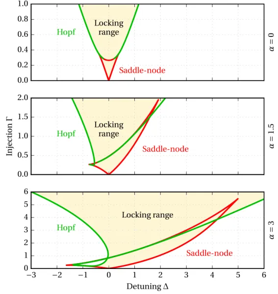
problem of synchronizing oscillators [Adler46]. The main lesson it teaches is that two regimes are possible: for |∆| <p1 + α2_{ΓEinj/|E|, the system converges toward a steady} state, called a phase locked solution. In this region, named the locking range, the frequencies of the two oscillators are the same. In our case, the output of the laser consists in a single wavelength, controlled by the injected field. Here we see clearly that as announced in the previous section, the linewidth enhancement factor plays a key role, as it widens the locking range by a factor p1 + α2_{. Now, when leaving the} locking region, the steady state disappears in what is called a saddle-node bifurcation, and the phase starts to experience a monotonous drift. For our laser, there are two different wavelengths in the output, the one of the injected signal, and the one of the laser, which will be slightly pulled toward the injected wavelength because of the phase drift [Armand69;Blin00].

Beyond the Adler equation

However, this analysis is only valid in the very particular situation of low injection, and considerably different behaviors can be obtained when a stronger field is injected into a laser. Indeed, the shape of the locking range becomes more complex, the unlocking may be different, and peculiar spectral properties can appear [Blin03;Wieczorek05].

For instance, unlocking can happen through a Hopf bifurcation, which consists in growing oscillations around the now unstable equilibrium point [Simpson97]. It has been proposed to use these oscillations, sometimes referred as "period-one" (or P1) as source of easily tunable microwave signal [Zhuang13; Hung15]. Indeed, their period depends on the injection rate and frequency detuning. More complex outputs may include spiking regimes with short pulses, and this has been proposed as an alternate way to enforce mode-locking in diode lasers [Moses76].

Also, chaotic regimes exist outside of the locking region, so that the injected semiconductor laser is a convenient device for the generation of wide-band chaotic spectrums. Furthermore, it has been shown that the chaotic regimes of two identical lasers can be synchronized using injection of light from one to the other [Murakami03;

Kim06]. This phenomenon of chaotic synchronization is widespread in dynamical systems [Pikovsky97], but particularly interesting in semiconductor lasers, as it has potential uses in secure chaotic communications [Sciamanna15].

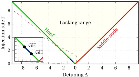
One important tool in the theoretical study of the possible behaviors are the bifurcation diagrams, which show the locus and type of the relevant bifurcations of the equilibrium with respect to the parameters of the system. They are often produced using numerical methods based on continuation algorithms. They allow to follow an equilibrium of the system while varying a parameter, but can also be used to follow