HAL Id: emse-03128555
https://hal-emse.ccsd.cnrs.fr/emse-03128555
Submitted on 2 Feb 2021
HAL is a multi-disciplinary open access
archive for the deposit and dissemination of
sci-entific research documents, whether they are
pub-lished or not. The documents may come from
teaching and research institutions in France or
abroad, or from public or private research centers.
L’archive ouverte pluridisciplinaire HAL, est
destinée au dépôt et à la diffusion de documents
scientifiques de niveau recherche, publiés ou non,
émanant des établissements d’enseignement et de
recherche français ou étrangers, des laboratoires
publics ou privés.
Detection of Behavioral Changes on Activities Daily
Routine in a Smart Home using Heatmaps
Cyriac Azefack, Raksmey Phan, Vincent Augusto, Guillaume Gardin, Claude
Montuy Coquard, Remi Bouvier, Xiaolan Xie
To cite this version:
Cyriac Azefack, Raksmey Phan, Vincent Augusto, Guillaume Gardin, Claude Montuy Coquard, et
al.. Detection of Behavioral Changes on Activities Daily Routine in a Smart Home using Heatmaps.
2020 IEEE 16th International Conference on Automation Science and Engineering (CASE), Aug 2020,
Hong Kong, France. pp.1019-1024, �10.1109/CASE48305.2020.9216898�. �emse-03128555�
An Approach for Behavioral Drift Detection in a Smart Home
Cyriac Azefack
1,2, Raksmey Phan
1, Vincent Augusto
1, Guillaume Gardin
2,Claude Montuy Coquard
2,
Remi Bouvier
2and Xiaolan Xie
1, Fellow, IEEE
Abstract— With the global population growing older and more vulnerable, healthcare systems are considering new ap-proaches to maintain people autonomous in their own homes. Recent advances in pervasive computing technologies have opened up new opportunities to unobtrusively monitor human behavior at home. Sensors data related to the activities of daily living (ADLs) performed by the inhabitant can be collected and labeled manually or by using activity recognition algorithms. The purpose of this work is to propose an approach for detecting changes (drift) in the inhabitant behavior in order to detect potential changes in the health-state of the inhabitant. Based on unsupervised clustering, our approach use activity starting time and duration as key features to detect changes between time periods. Variations from one behavior to another one can be identified for subsequent review or intervention by a healthcare professional. The relevance and the nature of the change are asserted using the clustering validation metric called Silhouette. Case study experiments on real life and simulated datasets suggest that some user’s behavior can go through smooth or abrupt changes and that these changes can be highlighted using our approach.
I. INTRODUCTION
Industrialized countries are experiencing deep social and economic changes affecting their demography. According to the United Nations Population Fund (UNFPA) [1], the global population of elderly people aged 60+ years is expected to rise to around 2 billion by 2050, outnumbering the number of children. Such demographic changes will lead to a growing demand for assistance requiring public and private healthcare. Furthermore, elderly people need a unique care approach due to the complexity of their health situation. The increasing shortage in healthcare workers could have a huge impact on the healthcare economy. To avoid this situation, the current healthcare system must move from a reactive paradigm to a more proactive one such as prevention through health monitoring at home.
Recent advances in pervasive computing technologies have opened up new opportunities such as smart homes. A smart home refers to a residence equipped with non-intrusive sensors that detect specific events happening in the residence (e.g., motion, door openings, sleep duration, etc.). Information related to the Activities of Daily Living (ADLs) performed by the inhabitant is collected to monitor
*This work was supported by the french organization EOVI MCD
1Cyriac Azefack, Raksmey Phan, Vincent Augusto and Xiaolan Xie are
with Mines Saint-Etienne, Univ Clermont Auvergne, CNRS, UMR 6158 LIMOS, Centre Ingenierie et Sant´e, F-42023 Saint-Etienne France. Emails: {cyriac.azefack, raksmey.phan, augusto, xie}@emse.fr
2Cyriac Azefack, Guillaume Gardin, Claude Montuy Coquard, Remi
Bouvier are with the french health assurance company EOVI MCD, 60 rue Robespierre 42012 Saint-Etienne France. Emails: {guillaume.gardin, claude.montuy-coquard, rbouvier}@eovi-mcd.fr
its behavior over time. Elderly people behavior tend to be consistent over time. Gerontologists believe detecting long-term behavioral changes (Behavioral Drift) on activities of daily living (ADLs) (bathing, sleeping, eating, ...) and Instrumental ADLs (IADLs) (cooking, taking medication, use phone,...) is the best procedure to prevent deterioration of the health condition [2], [3]. Behavioral drifts may indicate a need for more effort to perform everyday tasks or reveal the onset of disorders like Alzheimer or dementia.
Extensive research has been reported on smart homes on behavior monitoring with different applications such as behavior and activity recognition [4]–[7], anomaly detection [8]–[10] and behavior prediction [11]–[13]. The scientific challenge related to anomaly detection consists in differenti-ating the inhabitant “normal” behavior from the “abnormal” one. By using low-level sensors (movements and door entry points sensors) to monitor the activities of elderly people living at home, [10] proposed an approach to detect and predict abnormal behavior using visualization, clustering and neural networks. The purpose was to alert the elderly caregiver in case an abnormality has been detected or is predicted in the near future which can be seen as short-term anomalies. [8] defines outliers or anomalies activities as an activity with extremely high or low systolic value as compared to the rest of the data using the z-score. As for most work done on anomaly detection, [8], [10] focus on abnormal events, or short-term changes but not on behavior drift which can be seen as a long-term change. Changes in the inhabitant behavior are not necessarily abnormal behaviors and on the other side, a succession of abnormal behaviors can be the sign of a new behavior emerging and these are not covered in the present literature on smart homes.
The literature is scarce regarding long-term behavioral changes or behavioral drift detection in the context of smart homes. However, drift detection in business processes using process mining or machine learning has been tackled in [14]– [17]. Regarding human behavior as a process of activities, process mining techniques to detect drift could be applied in this context. [15] proposed an approach to detect drift using clustering: by comparing traces from a business log, trace clustering allowed the detection of mainstream and deviating behaviors in a process. Similarly, [18] proposed an approach to detect behavioral drifts in a smart home. The idea was to analyze the behavioral impact of health events. The method consisted of segmenting the activity event log in weeks and comparing the different weeks to the first week (considered as the normal behavior). They used the symmetric Kullback-Leibler (KL) divergence distance metric
and an arbitrarily chosen threshold, a distance above the threshold would signal drift in the behavior. This approach gave outstanding result when they correlate the behavioral drift detected to related health events. A major limitation of this work is the constraint of having a “reference week” to perform the comparison.
In this paper, we focus our attention on activities of daily living (ADLs) in order to detect behavioral drift of the inhabitant living in the smart home. Historical data of the inhabitant is used to identify the different behaviors without any assumptions on their nature. Detection of behavior drift relies on the clustering of time periods to differentiate mainstream and deviating behaviors.
This paper is organized as follows. Section II briefly introduces necessary definitions. Section III describes our behavioral drift detection approach. An application of our method on synthetic generated datasets is presented in Sec-tion IV and an applicaSec-tion on a real-life case study is presented in Section V. Conclusions and perspectives are given in Section VI.
II. PRELIMINARIES
In this section, we introduce the main concepts and notations used in this paper.
Definition 2.1 (Event): An event e is denoted as the tuple e = (a, t, d) where a is the event activity, t the starting timestamp of the event and d its duration. Let E be the event universe, i.e. the set of all possible event identifiers.
Definition 2.2 (Event Log): An event log L = he1, e2, ..., eni is a finite sequence of events L ⊆ E∗ such that each event appears at most once in the entire log. Definition 2.3 (Activity Event Log): An activity event log La = he1, e2, ..., eni is an event log such as ∀ e ∈ La, activity(e) = a. The activity event log describes the behavior of the inhabitant for a specific activity.
Definition 2.4 (Time Window Log): A time window log (or just time window) wi= hei1, ei2, ..., einii is an event log
with nievents, extracted from an input event log L (wi⊆ L) such that the sublog duration is constrained by a window size parameter Tw (tini− ti1≤ Tw).
Definition 2.5 (Time Window Similarity Matrix): Let W be a set of time windows, MW = (W ×W) → [0, 1] denotes the similarity matrix of W. For time windows wi, wj∈ W, MW(i, j) represents the similarity between the time windows wi and wj.
Definition 2.6 (Time Window Clustering): Let W be a set of time windows. A time window cluster over W is a subset of W. A time window clustering T C ⊆ P(W) (where P(W) denotes all the possible subsets of W) is a set of time window clusters over W. We assume every time window to be part of one unique cluster, i.e. clusters overlap is not allowed.
The input data of our problem is an ordered sequence of events describing the activities done by the smart home inhabitant during a certain time period. To do so, the smart home is equipped with multiple sensors recording the life of the inhabitant. The data collected are sensors data, which
is an event log of sensors activation and deactivation and is complex to use for behavioral drift detection. These data are either manually annotated using activities label or labeled by using activity recognition algorithms [4], [6], [19] to obtain activity event logs.
To reduce the complexity of the problem we focus on each activity’s behavior independently, i.e. the behavior changes related to multiple activities are beyond the scope of this paper. We analyze behavior drifts on each activity to catch how their starting time and/or duration change through time. The method presented in this paper only deals with activities event log (c.f. Definition 2.3).
In [20], authors identified four classes of drifts in business process behaviors: (i) Sudden Drift (sudden substitution of an existing behavior with a new one); (ii) Recurring Drift (a set of behaviors reappear after some time); (iii) Gradual Drift (gradual substitution of an existing behavior with a new one); (iv) Incremental Drift (substitution of a behavior with a new one through intermediate behaviors). Recurring and incremental drift can be modeled as successive sudden drifts. In this paper, we assume that the period of change between behaviors is a fixed point and gradual drift detection is beyond the scope of this paper.
Time is a key point in our daily life and is a fundamental source of information on the inhabitant lifestyle. In their work, [9], [10] used activities start time and duration as features to discriminate normal and abnormal behaviors. Multiple aspects of the inhabitant lifestyle can be subject to changes but since we focus on each of the inhabitant activity independently, we are going to describe behavior change as changes on either of these two features : (i) activity starting time (changes on an activity starting time, e.g. when the inhabitant starts going to bed later than usual or changes his medication time); (ii) activity duration (changes on an activity duration, e.g. when the inhabitant sleeps less or take more time to perform some ADLs such as bathing, cooking, ...).
III. METHODOLOGY
In this paper, we propose a new approach to detect changes in the inhabitant lifestyle manifested as sudden drifts over a period of time. To detect behavior drifting point in the input activity event log, we split the event log into overlapping time window logs of fixed duration Tweach, as shown in Figure 1. The starting time window w0 contains events that occurred between t0 ≤ t ≤ t0+ Tw. The sliding interval duration is Tp: we map it to the circadian rhythm (24 hours) [21]. The i-th time window contains events that occurred between t0+ i.Tp ≤ t ≤ t0+ i.Tp+ Tw. The time window logs created can contain overlapping data; an event can belong to more than one time window log. In the case presented in Figure 1, we have one drifting point between Behavior 1 and Behavior 2. Such sudden drift is presented in Figure 2. A. Time Windows Clustering
Clustering algorithms partition data into a certain number of groups (clusters, subsets, categories). The most common
t0 Behavior 1 t0+ i.Tp Drifting Point Behavior 2 t w0 Tw Tp w1 wi wi+1
Fig. 1: Time window logs extraction .
time
B1
B2
Drifting Point
Fig. 2: Behavior Drift over time
definition of clustering describes a cluster by considering its internal homogeneity and external separation meaning that data points in the same group should be close to each other, while data points in different groups should not. The proximity of data points can be expressed in different ways. Given an input activity event log La on the activity a, let Wa be the set of time window logs extracted from La using a sliding time window. When the clustering is performed, a change is identified when two consecutive time window logs wi and wi+1 are put in different behavior clusters. In order to achieve the clustering, we need a proximity metric (distance/similarity) between time windows. The work of [22] outlines three different approaches to compute data point proximity in this context: (i) raw-data-based, (ii) features-based and (iii) model-features-based. The model-features-based approach assumes that the data follow a predefined model and the distance/similarity metric is defined on how close the data point suits the model. Since we have no assumption on the model behind our data, this approach cannot be used in this context. We implemented the two approaches left, features-based clustering and the raw-data-based clustering. To validate the clustering quality, we used the Silhouette Index(SI) metric as described in III-C. The raw-data-based approach gave significantly better results than features-based, so we decided to present here only the successful approach described in III-B.
B. Raw-data-based clustering
In this approach, the similarity between time windows is computed from raw data using a similarity metric. Then, the clustering relies on the Markov Clustering (MCL) algorithm [23], which has been successfully applied in other fields like computational genomics [24] and process mining [15], [16]. Such algorithm is a fast and scalable cluster algorithm for graphs, where each node is a data point (time window) and the edge’s weights are the similarity between data points. In our case, the input of the MCL algorithm is a time window similarity matrix (Cf. Definition 2.5). The computation of
the similarity matrix is separated from the actual clustering, hence different methods can be used for both parts.
1) Similarity matrix computation: Let wi = hei1, ei2, ..., einii be a time window with ni
events. Depending on which aspect of the activity we want to look at (starting time/duration) we extract the time window distribution array Di (relative starting times / durations) from wi. If we consider the activity starting time aspect, Di = htri1, tri2, ..., trinii (with t
r
ij the relative timestamp of the event eij), but if we consider the activity duration aspect, Di = hdi1, di2, ..., dinii (with dij the
duration of the event eij). The similarity between time windows is defined on how close the distributions Di are.
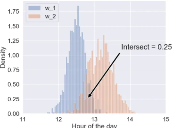
We propose to compute the distance between the distri-bution using histograms intersection. This method is widely use for images clustering and classification [25]. It calculates the similarity of two probability distributions issues from empirical data with possible value of the intersection lying between 0 (no overlap) and 1 ()identical distributions). Given a pair of time window distribution arrays Di and Dj, of time windows wi and wj, we compute their respec-tive normalized histograms Hi and Hj, each containing n bins, the similarity sim between wi and wj is defined as sim = Hi ∩ Hj= Pnk=1min(Hi(k), Hj(k)). Figure 3 shows an example of histogram intersection of an activity starting time on two different time windows w1and w2. The activity has a earlier starting time during w1than w2, which gives a similarity score of 0.25.
Fig. 3: Example of histogram intersection
2) Graph clustering: Once a similarity matrix is built using the similarity between all time window logs, it is represented as a weighted graph where each node is a time window and edges are the similarity value between time windows. The way this graph is built makes it suitable to
graph clustering algorithms such as the MCL algorithm. For detailed information on the MCL algorithm please refer to [24].
C. Clustering Validation
Since the inhabitant behavior changes are not known a priori, the validity of the changes detected by our approach should be assessed using appropriate criteria, irrespective of the clustering methods. As one of the most used metric for clustering, the Silhouette Index [22] has been selected to assess the clustering quality regardless of the chosen algorithm.
The distance metric here is the opposite of the similarity metric defined earlier: dist(wi, wj) = 1 − sim(wi, wj). For each time windows w ∈ W, let u(w) be the average distance between w and all other time windows within the same cluster. It is a measure expressing how well the assignment of w to its cluster is. Let v(w) be the smallest average distance of w to all points in any other cluster, of which w is not a member. It expresses the dissimilarity between w and the other clusters. A time window Silhouette index is defined as s(w) = max(u(w),v(w))v(w)−u(w) with −1 ≤ s(w) ≤ 1. Lower values of u(w) imply the time windows is well matched to its cluster while higher values of v(w) means that w badly matches other clusters. So a good clustering means a value of s(w) close to 1. A value of s(w) close to -1 means that another cluster will be a better match to w. We define the Silhouette index SI of the clustering as the average Silhouette of all the time windows, so the closer SI is from 1, better is the clustering.
IV. NUMERICAL EXPERIMENT
To assert the validity of our approach, it is necessary to compare the drifts detected to the ones actually present in the inhabitant’s behavior. Due to the lack of that kind of data, we decided to generate synthetic datasets with induced drift on different levels, from mild and smooth drifts to severe and abrupt ones.
A. Dataset Generation
The goal here is to model the behavior of the inhabitant in the house for a specific activity. However, a model based on the “average” behavior for an activity would be repetitive and would not look natural. For example, the activity Eating can be done in the morning (Breakfast) or in the evening (Dinner) and these ways of performing the same activity can have their own behavioral changes. To build a more realistic and not fixed behavior model of a resident, we introduce the concept of daily pattern: one way of performing the activity on a daily basis which has properties that distinguish it from others (e.g., breakfast, lunch, dinner).
For an activity ai, we assume that the inhabitant has a set of daily patterns R = {r1, ..., rn}. Thus, each day a subset of R is performed according to each daily pattern respective properties and this subset is called a daily behavior. A daily behaviorQ ⊆ R is an ordered subset of daily patterns char-acterizing the behavior of the inhabitant during a day. For ex-ample, the set of daily patterns {breakf ast, lunch, dinner}
is a daily behavior describing the days when the inhabitant had these three meals, but he could have another daily be-havior like {breakf ast, early dinner} describing the days when he missed lunch but took an early dinner.
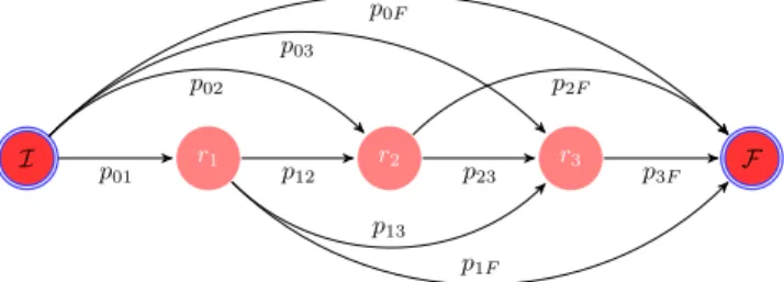
Let Q = {r1, ..., rk} be a daily behavior of the inhabitant. We use a graph to model the execution of Q. Let GQ be the graph representing the daily behavior Q. It can be formally defined as the graph GQ with k + 2 states, k daily patterns plus an initial (I) and final state (F ).
The States I and F denote respectively the entry and the final state of the graph. Each transition exiting from the entry state denotes the probability of starting the day with a specific pattern, except for the transition to F which denotes the probability of doing none of the patterns of Q. An example of the graph representing a daily behavior with three daily patterns is presented in Figure 4.
I p r1 r2 r3 F 01 p02 p03 p0F p1F p12 p13 p2F p23 p3F
Fig. 4: Graph model of a daily behavior Q = {r1, r2, r3}
For the inhabitant overall behavior, we use a Markov chain graphas a simulation model as depicted in Figure 5. The node O is the entry node, it marks the beginning of the next day and the end of the previous one. Let assume our inhabitant has m different daily behaviors Qi (with 1 ≤ i ≤ m), depending on the timestamp t, the inhabitant has a probability pi(t) of performing the daily behavior Qi for the current day. After the daily behavior is performed, the day ends and a new one starts. To respect the Markov property we have : ∀t,Pm
i=1pi(t) = 1. The drift in the behavior is represented in pi(t); when the inhabitant changes his daily habits, the probability of the new daily behavior increases. So the behavioral drift is generated by tuning the evolution of the pi(t) with 1 ≤ i ≤ m.
start Q1<i<m
pi
1
Fig. 5: Markov graph of the simulation model
B. Design of experiment
Table I describes an example of an inhabitant eating habits . For instance, the breakfast habit occurs on average at 8h30am with a standard deviation of 15mn and the meal lasts on average 20mn with a standard deviation of 8mn.
TABLE I: Patterns of the eating behavior
Pattern Name Starting Time Dis-tribution Durationtion
Distribu-Breakfast Nt(8h30, 15mn) Nd(20mn, 8mn)
Lunch Nt(13h25, 30mn) Nd(40mn, 10mn)
Dinner Nt(18h50, 45mn) Nd(25mn, 5mn)
Brunch Nt(11h30, 15mn) Nd(20mn, 7mn)
Early Dinner Nt(17h30, 25mn) Nd(40mn, 10mn)
We consider the two daily behaviors Q1 = {Breakfast, Lunch, Dinner} and Q2 = {Brunch, Early Dinner} with the respective daily probability p1(t) and p2(t). We generate 200 event logs. Half of the logs (100 logs) do not have any behavioral drift (∀ t, p1(t) = p2(t) = 0.5). The other half of the logs have a probability function varying as shown in Figure 6. The evolution of the probabilities are based on sigmoid function which is supposed to describe the natural evolution of an inhabitant behavior through time. The closer p1(t) and p2(t) are at timestamp t = 0, milder is the drift and thus harder to detect. We choose a range of initial values for (p1(0), p2(0)) ∈ {(0.95, 0.05); (0.9, 0.1); ...; (0.55, 0.45)} to cover different levels of drift.
1.0 2.0 3.0 4.0 5.0 6.0 7.0 8.0 9.0 10.0 11.0 12.0 0.2 0.4 0.6 0.8 1.0 Drifting Point months probability p1(t) p2(t)
Fig. 6: Daily behavior probability evolution over time
C. Results
The first experiment intends to test the ability of our method to detect a drift among the set of event logs. We used a sliding window size of three weeks (Tw= 21 days). Results presented in Table II allow for validation of the quality of our approach. Each row corresponds to a type of dataset (with or without drift), each column corresponds to the classification done by our approach. Among 200 datasets treated, 100 with drift and 100 without, 162 are correctly classified and 38 are not, which gives an F1-score of 0.79.
TABLE II: Drift detection on synthetic datasets Detected
Yes No
Actual
Yes 71 29 No 9 91
We evaluate the quality of the drift detected using the Silhouette metric and the results are depicted in Figure 7. The distribution is quite narrow and the mean silhouette value is
0.76. This means that on average, the quality of the drift detected by our approach on these datasets is asserted.
Fig. 7: Silhouette distribution of the drifts detected among synthetic event logs
V. REAL-LIFECASESTUDY
Experiments were performed on the Aruba dataset [19]. It describes an elderly woman carrying out daily activities in a smart home, without any kind of supervision or scripted scenario. The dataset lasts for 220 days and 11 activities were recorded. Each activity was processed separately using a sliding window size of three weeks (Tw= 21 days). We applied the behavioral drift detection method for the activities starting time and the activities duration. Among the changes detected, there is a drift detected on the “Eating” activity starting time as shown in Figure 8 with a silhouette value of s = 0.53.
(a) Behavior drift over time
(b) Behaviors density distribution
Fig. 8: Drift Detection results for the “Eating” activity starting time on Aruba Dataset
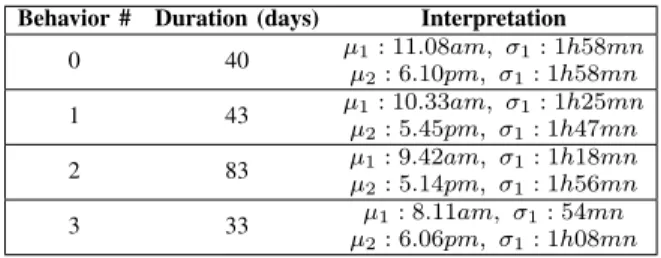
The Figure 8a depicts the way the inhabitant eating behaviors appear over time. The Table III gives more details on the different eating behaviors. We can notice that over time, she had her first meal of the day earlier and earlier: from an average of 11.10am on Behavior#0 to an average
TABLE III: Different behaviors detected on the “Eating” activity in the Aruba dataset
Behavior # Duration (days) Interpretation 0 40 µµ1: 11.08am, σ1: 1h58mn 2: 6.10pm, σ1: 1h58mn 1 43 µ1: 10.33am, σ1: 1h25mn µ2: 5.45pm, σ1: 1h47mn 2 83 µµ1: 9.42am, σ1: 1h18mn 2: 5.14pm, σ1: 1h56mn 3 33 µ1: 8.11am, σ1: 54mn µ2: 6.06pm, σ1: 1h08mn
of 8.11am on Behavior#3. The same goes for her second meal, from an average of 6.10pm on Behavior#0 to an av-erage of 5.14pm on Behavior#2, and for the last behavior detected she went back to eating at 6.06pm. This can also be observe on the behavior density distributions on Figure 8b, we can notice that the behavior density distributions are shifting to the left (for earlier starting time).
VI. CONCLUSIONS ANDPERSPECTIVES
Human behavior is a complex mechanism constantly subjects to variations due to biological and environmental factors. We proposed in this paper a novel approach to detect behavioral drift in the activities performed by a resident. The focus was in clustering time window logs extracted from the inhabitant activity log. The two main features used for the clustering are activity starting time and duration. The clusters detected allowed the identification of the inhabitant different behaviors.
Experiments based on synthetic datasets with induced drift and a real-life case study show that inhabitant behavior is constant during a certain period of time and then change, and that change can be identified by our approach.
In previously published works [8]–[10], the focus is on de-tecting abnormal behaviors: short periods of time (an event, a day, ...) where the inhabitant behavior deviates from the “normal” behavior. Instead, our approach does not assume a “normal” behavior but try to identify the inhabitant different behaviors and thus the period of change between them. Moreover, our approach allows for an overall visualization of the inhabitant behavior changes through time.
A current limitation of the proposed approach is that the inhabitant activities are processed separately. In future work, we intend to analyze the drift on all activities at once. We will also investigate the addition of more features for the clustering of behaviors such as the inhabitant activity level (number of activities performed during a period of time) and the inhabitant idle time (time spent performing no activities). Further evaluation of the changes detected and their relationships to health or care intervention are also under consideration.
REFERENCES
[1] UNFPA and H. International, “Ageing in the Twenty-First Century A Celebration and A Challenge,” Tech. Rep., 2012.
[2] M. P. Lawton and E. M. Brody, “Assessment of Older People: Self-Maintaining and Instrumental Activities of Daily Living,” Gerontologist, vol. 9, no. 3 Part 1, pp. 179–186, sep 1969.
[3] W. A. Rogers, B. Meyer, N. Walker, and A. D. Fisk, “Functional Limitations to Daily Living Tasks in the Aged: A Focus Group Analysis,” Hum. Factors J. Hum. Factors Ergon. Soc., vol. 40, no. 1, pp. 111–125, mar 1998.
[4] E. Kim, S. Helal, and D. Cook, “Human activity recognition and pattern discovery,” IEEE Pervasive Comput., vol. 9, no. 1, pp. 48–53, jan 2010.
[5] A. Fleury, M. Vacher, and N. Noury, “SVM-based multimodal classification of activities of daily living in health smart homes: Sensors, algorithms, and first experimental results,” IEEE Trans. Inf. Technol. Biomed., vol. 14, no. 2, pp. 274–283, mar 2010.
[6] N. C. Krishnan and D. J. Cook, “Activity recognition on streaming sensor data,” Pervasive Mob. Comput., vol. 10, no. PART B, pp. 138–154, 2014.
[7] “Le syndrome de fragilit´e - Revue M´edicale Suisse.”
[8] G. Jain, D. J. Cook, and V. Jakkula, “Monitoring Health by Detecting Drifts and Outliers for a Smart Environment,” in Int. Conf. Smart homes Heal. Telemat. Book Title Book Editors IOS Press, 2006, pp. 114–121.
[9] F. Cardinaux, S. Brownsell, M. Hawley, and D. Bradley, “Modelling of behavioural patterns for abnormality detection in the context of lifestyle reassurance,” in Lect. Notes Comput. Sci. (including Subser. Lect. Notes Artif. Intell. Lect. Notes Bioinformatics), vol. 5197 LNCS. Springer, Berlin, Heidelberg, 2008, pp. 243–251.
[10] A. Lotfi, C. Langensiepen, S. M. Mahmoud, and M. J. Akhlaghinia, “Smart homes for the elderly dementia sufferers: Identification and prediction of abnormal behaviour,” J. Ambient Intell. Humaniz. Comput., vol. 3, no. 3, pp. 205–218, sep 2012.
[11] N. K. Suryadevara, S. C. Mukhopadhyay, R. Wang, and R. K. Rayudu, “Forecasting the behavior of an elderly using wireless sensors data in a smart home,” Eng. Appl. Artif. Intell., vol. 26, no. 10, pp. 2641–2652, nov 2013.
[12] A. R. M. Forkan, I. Khalil, Z. Tari, S. Foufou, and A. Bouras, “A context-aware approach for long-term behavioural change detection and abnormality prediction in ambient assisted living,” Pattern Recognit., vol. 48, no. 3, pp. 628–641, 2015.
[13] H. Mshali, T. Lemlouma, M. Moloney, and D. Magoni, “A survey on health monitoring systems for health smart homes,” Int. J. Ind. Ergon., vol. 66, pp. 26–56, jul 2018.
[14] R. P. C. Bose, W. M. Van Der Aalst, I. Zliobaite, and M. Pechenizkiy, “Dealing with concept drifts in process mining,” IEEE Trans. Neural Networks Learn. Syst., vol. 25, no. 1, pp. 154–171, jan 2014. [15] B. F. Hompes, J. C. Buijs, W. M. Van Der Aalst, P. M. Dixit, and
J. Buurman, “Detecting change in procebes using comparative trace clustering,” in CEUR Workshop Proc., vol. 1527, 2015, pp. 95–108. [16] B. Hompes and J. Buijs, “Discovering Deviating Cases and Process
Variants Using Trace Clustering,” Tech. Rep., 2015.
[17] J. Gama, P. Medas, G. Castillo, and P. Rodrigues, “Learning with Drift Detection.” Springer, Berlin, Heidelberg, 2010, pp. 286–295. [18] G. Sprint, D. Cook, R. Fritz, and M. Schmitter-Edgecombe,
“Detecting Health and Behavior Change by Analyzing Smart Home Sensor Data,” in 2016 IEEE Int. Conf. Smart Comput. SMARTCOMP 2016. IEEE, may 2016, pp. 1–3.
[19] D. Cook, “Learning Setting-Generalized Activity Models for Smart Spaces,” IEEE Intell. Syst., vol. 27, no. 1, pp. 32–38, jan 2012. [20] R. P. C. J. C. Bose, W. M. P. Van Der Aalst, I. ˇZliobaite,
M. Pechenizkiy, B. R. B, V. D. A. W.M.P.a, ˇZ. I.a, P. M.a, R. P. C. J. C. Bose, W. M. P. Van Der Aalst, I. ˇZliobait, and M. Pechenizkiy, “Handling concept drift in process mining,” in Lect. Notes Comput. Sci. (including Subser. Lect. Notes Artif. Intell. Lect. Notes Bioinformatics), vol. 6741 LNCS, 2011, pp. 391–405. [21] P. H. Redfern, J. M. Waterhouse, and D. S. Minors, “Circadian
rhythms: Principles and measurement,” 1991.
[22] T. Warren Liao, “Clustering of time series data - A survey,” pp. 1857–1874, nov 2005.
[23] S. Van Dongen, “A New Cluster Algorithm for Graphs.”
[24] A. J. Enright, “An efficient algorithm for large-scale detection of protein families,” Nucleic Acids Res., vol. 30, no. 7, pp. 1575–1584, apr 2002.
[25] A. Barla, F. Odone, and A. Verri, “Histogram intersection kernel for image classification,” in Proc. 2003 Int. Conf. Image Process. (Cat. No.03CH37429), vol. 2. IEEE, pp. III–513–16.