Near Optimum Low Complexity Smoothing Loops for Dynamical Phase Estimation—Application to BPSK Modulated Signals

HAL Id: hal-01180826

https://hal.archives-ouvertes.fr/hal-01180826

Submitted on 4 Nov 2015

HAL is a multi-disciplinary open access archive for the deposit and dissemination of sci-entific research documents, whether they are pub-lished or not. The documents may come from teaching and research institutions in France or abroad, or from public or private research centers.

L’archive ouverte pluridisciplinaire HAL, est destinée au dépôt et à la diffusion de documents scientifiques de niveau recherche, publiés ou non, émanant des établissements d’enseignement et de recherche français ou étrangers, des laboratoires publics ou privés.

Dynamical Phase Estimation-Application to BPSK

Modulated Signals

Jianxiao Yang, Benoit Geller

To cite this version:

Jianxiao Yang, Benoit Geller. Near Optimum Low Complexity Smoothing Loops for Dynamical Phase Estimation-Application to BPSK Modulated Signals. IEEE Transactions on Signal Processing, Institute of Electrical and Electronics Engineers, 2009, pp.3704-3711. �10.1109/TSP.2009.2021452�. �hal-01180826�

Abstract—This paper proposes a near-maximum a posteriori smoothing algorithm for the dynamical carrier

phase estimation of coded quadrature amplitude modulation (QAM) signals. This low-complexity near-optimum smoothing is obtained by averaging phase-locked loops (PLLs) with possibly the aid of the decoded a posteriori information. The proposed code-aided smoothing algorithm performs near the off-line Bayesian and hybrid Cramer-Rao bounds (BCRBs and HCRBs) of interest. It has a gain of several decibels compared to the conventional on-line loop and is able to track frequency offsets.

Index Terms—Bayesian Cramer-Rao Bound (BCRB), Code-Aided (CA), Data-Aided (DA), Dynamical Phase

Estimation, Hybrid Cramer-Rao Bound (HCRB), Maximum A Posteriori (MAP), Non-Data-Aided (NDA), Smoothing Phase-locked Loops (S-PLL)

I. INTRODUCTION

odern communications systems have to cope with more and more stressing conditions (low signal-to-noise ratios (SNRs), high data rate). As phase estimation is processed at the front-end of digital receivers, phase errors rapidly degrade the overall performance of communication systems and consequently phase synchronization has become one of the most critical tasks that a receiver has to operate. To solve this challenging phase synchronization problem, many signal processing techniques have been proposed. Among Bayesian methods, [1] proposed a non-coherent method based on a truncated memory, [2]-[4] executed message passing algorithms based on factor graphs and the algorithms

Names

Near-MAP Smoothing Loops for Code Aided

QAM Dynamical Carrier Phase Estimation

proposed in [5],[6] are based on the variational Bayesian methods. [7] composed a partical filtering with a phase-locked loop technique and found some interest to partical filtering when there are abrupt changes in the phase trajectory. A BCJR based Gaussian sum smoother was proposed in [21] for convolutional turbo code aided dynamical phase estimation, and was derived by extending the original BCJR algorithm [26] to the case of joint phase estimation and decoding. However, in the general case, Bayesian methods are far more complex to implement than deterministic methods and thus deterministic phase algorithms have been employed so far in real systems. The most commonly used deterministic methods are based on the EM algorithm [8],[9] or on gradient-like phase locked loops (PLL) techniques. PLL are traditionally known as low-cost algorithms that lead to a good asymptote performance for on-line estimation [10]. Their performance can even be improved at low SNRs within the turbo-receiver concept [11]-[13]. Rather than considering actual on-line estimation for which estimated values only depend on past observations, one may also consider off-line estimators involving both past and future observations; such a data block approach is a very natural way to proceed, as modern systems use error correcting codes. Bayesian and hybrid Cramer-Rao bounds (BCRBs and HCRBs), associated to this dynamical phase synchronization problem, have been considered in some recent contributions [14]-[17] and they allow to measure the performance of such algorithms; they clearly show the superiority of the off-line approach, compared to the on-line approach. Contrarily to the performance of [11]-[13] limited by the on-line bound, [17] analyzed a smoothing PLL (S-PLL) algorithm based on two on-line PLLs that was proposed without any performance evaluation in [18]. [17] derived the S-PLL algorithm for a non-coded BPSK system and it is well known that it is not difficult to achieve synchronization in such a context. [19] and [20] extended the study of the S-PLL algorithm to other telecommunication formats.

In this paper, we extend the analysis of the S-PLL to the useful case in practice of channel encoded QAM modulated systems. We derive our algorithm from the definition of the code-aided (CA) a posteriori probabilities (APPs) and we then compare its performance with Cramer-Rao bounds of interest. However, we have to point out that the computation complexity of the true maximum a posteriori (MAP) algorithm for the CA scenario exponentially increases with the block length and is impossible to achieve in practice. Nevertheless, the near-MAP algorithm derived via some approximations is able to reach the lower bound over a very wide SNR range. Moreover, we prove the asymptotic convergence of the algorithm towards the Bayesian Cramer-Rao bound illustrate. We also illustrate the respective

The rest of the paper is structured as follows. The system model is described in Section II. After briefly reviewing the MAP estimation principle in Section III, a code-aided near-MAP estimation framework is derived in Section IV. In Section V, we prove the asymptotic convergence of the algorithm. Some practical considerations are then discussed in the next section and numerical results are presented in section VII, where we illustrate the algorithm performances and compare them to the Cramer-Rao bounds of interest. Finally, in Section VIII, some concluding remarks are made.

II. SYSTEM MODEL

We consider the transmission of symbols sl belonging to a constellation set SM



s1, ,sM



(such as M-PSK or M-QAM) over an additive white Gaussian noise (AWGN) channel, additionally affected by some carrier phase offsets

l

 . The sequence of symbols are stacked in the symbols vector



1, ,



T L

s s



s and the phase offsets are stacked in the

vector



1, ,



T L

 



θ .Assuming that the timing recovery is perfect, the sampled baseband signal



1, ,



T L

y y



y does not

suffer from any inter-symbol interference (ISI) and can thus be written as





l l

j j

l l l l l l

y s e  n a jb e n, (1) where at time l, slis the

th

l transmitted complex symbol, l is the perturbing phase that must be estimated and the last

term nl in the right-hand side of (1) is a circular Gaussian noise with zero-mean and variance

2

n

 .

For the code-aided system, we assume that K bits are encoded into a codeword 1, ,2 , 



| 1, , 2



K N v

c c c v

  

c c of N

bits which are further mapped as a constellation vector s c

 

v 



s1

 

cv , ,sL

 

cv



. In this scenario, the independent and

identically distributed (i.i.d.) law among the transmitted symbols does not hold any more, instead, the i.i.d. law holds among all the 2K _{elements of the codebook. So the conditional probability density based on the known phase vector θ}

can be written as   2     2



 





 



2  2 2



 



2 2 2 1 1 1 1 Re 1 1 | | , | , exp exp 2 . 2 K K L K _L jl l l v l v l v v v v K v v n v l n n y s e s y p p p p p                            _{  } _{  }      





 

c c y θ y c c θ c c y s s c θ s s c (2) We now consider the phase model. Due to the imperfections of the oscillator, the receiver suffers from jitter. Moreover, due to the lack of knowledge about the transmitter’s clock, there exists a constant frequency shift in the

receiver’s clock. This results on a classical Brownian phase model with a linear drift 1

l l wl

     , (3)

where at time l, wl is Gaussian distributed with zero mean and variance

2

w

 ,  is the unknown constant frequency offset (linear drift) and l is the unknown phase offset.This model [20]-[22] has been widely used to describe the

behavior of practical oscillators for which the frequency is randomly perturbed. The corresponding conditional probability can be written as

   1 2 1 2 1 | exp 2 2 l l l l p             _{ }          . (4)

III. MAPESTIMATION AND CONDITIONAL GRADIENT ASCENT ALGORITHM

The maximum a posteriori (MAP) estimation of the phase vector θ given the observation yis given by

     

ˆ _{arg max ln p ,   arg max ln p | lnp }

θ θ

θ y θ y θ θ , (5)

where p y θ , may also be expressed as

 ,  , , 

p 



p

s

y θ y θ s . (6)

Computing ˆθ is usually not a trivial problem and one can consider the following methods.

First-order Optimality Condition: The solution of (5) must also satisfy the following necessary condition of optimality   ˆ lnp , 0  θ y θ _{θ θ} , (7) where 1 , , T L         _{ }   

θ . (7) defines therefore L necessary conditions of optimality.

Gradient Ascent Optimization: Consider the following iterative algorithm 1. Pick l1, ,L 2. Update ˆθ as follows ˆ 1 ˆ 



 

ˆ 



ln , i i i m m m p      _{  }   y θ , (8)

 1   ˆi ˆi l l   _ _, lm (9) where 0.

3. Repeat 1 and 2 until convergence.

It is easy to see that this algorithm is nothing but a conditional gradient ascent algorithm. By definition, _θˆf _{is a fixed}

point of this algorithm iff

 

ˆ ln , f 0 m p   _  y θ , m (10)

i.e., any stationary point of lnp y θ , is a fixed point of the algorithm. Comparing with (7), we therefore see that the MAP estimate ˆθ is necessarily a fixed point of the above algorithm.

IV. DERIVATION OF THE NEAR-MAP CODE AIDED ALGORITHM

For this particular problem of estimating time-varying phase offsets, the model in (1)-(4) implies that

  2     2



 



  1 1 1 ln | ln | , , ln | , , K K _L v v l l l v l v v v l p p  p p y s s   p           _   _ _     _   



 

 

 y θ y c c θ c c c c c , (11)    1  1 2 ln ln ln | L l l l p p p _   



θ . (12)

Based on this model, we now derive the explicit expression of the error-term used by the gradient ascent algorithm

 

ˆ





ˆ

 

ˆ

lnp , lnp | lnp

  

θ y θ _{θ θ} θ y θ _{θ θ} θ θ _{θ θ} (13)

Taking (1)-(4) into account, we get for any index m such that 1 m L, the error-term considered in the gradient

ascent algorithm (see details of the calculus derived in the Appendix)

  ˆ   ˆ   ˆ ln , ln | ln , m m m p p p             θ y θ _{θ θ}  θ y θ _{θ θ}  θ θ _{θ θ} ₍₁₄₎ where      



 



2 ˆ 1 ln | , , ln | ln | Pr | , , K m m m v m v m v m m y s s p p                 θ _{θ θ} _



_ c y θ y θ c c y θ (15) and     1 1 ˆ 2 ln 2 ln m m m. m m p p                 θ _{θ θ} _ θ θ (16)

 



 



 



 



 



 



  2 1 1 1 1 2 2 1 1 2 2 1 1 1 1 1 ln | , , Pr | , , , 1 ln | , , ln | , , 1 1 Pr | , , Pr | , , , 1 2 2 ln Pr | , , K K K v v v m m m v m m m m v m m m v m v v m v m L v y s s m y s s y s s m L y                                            _   _ _   _           







c c c y θ c c c c y θ c c y θ c c y θ



 



2 1 | , , , . K L L L v L v L s s m L              _  _{ }  _ 



c (17)

All these derivatives are too hard to use in practice because they all involve an exponential number of sums. We thus propose the following method to find a good approximation of these derivatives. From (17), the terms containing an exponential number of sums can be further expressed as follows

 



 



 







 



 





    2 1 2 1 2 1 1 ln | , , Pr | , , ln | , , Pr , | , , ln | , , Pr , | , , , K K K v m m m v m v v m m m m v m v m m v v m M m m i m v m m v m i v i m y s s p y s s s s p y s s s s s s                                   







c c c c c y θ c c c c y θ c c c y θ (18) where





1, if 0, otherwise. v m i m i s s s s _  _{ }   c c (19) Thus  



 



 





   





2 1 2 1 1 2 1 ln | , , Pr | , , ln | , , Pr , , | , , 2 Im Pr | , , , K K m m m m v m v v m M m m i m v m m v m i i v m j M m i m i i n y s s p y s s s s s s y s e s s                              







c c c y θ c c c y θ y θ (20) where   2



 



2



 



  1 1 Pr | , , Pr , , | , , Pr , | , , K K v m i v m m v m i v m m v m i v v s s  s s s s  s s   s s    y θ 



cc  c  y θ 



cc  c y θ c c  . (21)

The term Pr



smsi| , ,y θ



in (21) is exactly the a posteriori probability (APP) of the code-aided scenario. Generally, the calculation of Pr



smsi| , ,y θ



is NP hard due to 2

K _{sums involved. However, if we consider the term}

 

Pr smsi| , ,y θ as the decoded information, there do exist tractable decoding algorithms for approximate and even

approximate value of Pr



smsi| , ,y θ



for turbo codes and low-density parity-check (LDPC) codes. Inserting (20) into (17), we can further modify our algorithm as below

 





   





 





1 2 2 2 1 1 1 2 1 2 1 2 Pr | , , Im , 1 1 , 1 2 2 Pr | , , Im L + , , M j i i i n F B m m m M j L L i L i i n s s y s e m m L s s y s e m L                          _{   }              





y θ y θ (22)

where the terms defined as

   





2 1 2 1 Pr | , , Im m M F j m m m i m i i n s s y s e            



 y θ (23) and    





2 1 2 1 Pr | , , Im m M B j m m m i m i i n s s y s e            



 y θ (24)

can be regarded as first order PLL outputs aided with the decoded information



Pr



smsi| , ,y θ





,

 F m

 and  B m

 being respectively updated in the increasing (Forward) and decreasing (Backward) time directions. The physical meaning of (22) can thus be interpreted as follows; for the first position m1, the MAP estimator is estimated from 2 with a

backward PLL and for the last position mL, the MAP estimator is estimated from L1 with a forward PLL; for the middle range positions 1 m L, the MAP phase estimator averages the values of the forward and of the backward

PLLs. Since in practice it is impossible to know the actual phase valuesm1, m, and m1 in the forward and backward loops defined in (25)-(26), we replace these true phase values by their estimates

    _{ }  





    _{ }  





1 1 2 ˆ 1 2 1 2 ˆ 1 2 1 ˆ ˆ _{Pr | , , Im ,} ˆ ˆ _{Pr | , , Im .} F m B m M F F j m m m i m i i n M B B j m m m i m i i n s s y s e s s y s e                                 _{  } 





y θ y θ (25)

Then the so-called smoothing PLL (or S-PLL) [17],[19] can be written as

    _{ }  





   





  _{ }  





2 1 2 ˆ 2 2 1 1 1 / 2 ˆ 1 2 1 2 ˆ _{Pr | , , Im} ˆ_{, 1,} 1 ˆ ˆ ˆ _{, 2 1,} 2 2 ˆ _{Pr | , , Im} ˆ_{, .} B F L M B j i i i n F B F B m m m M F j L L i L i i n s s y s e m m L s s y s e m L                                  _{   }         





y θ y θ (26)

Note that for a BPSK non coded system, (26) just reduces to equation (18) of [17]. The expression “Smoothing loops” stems from the estimation procedure; the S-PLL encompasses one classical forward PLL and one backward

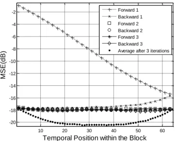
PLL working in the reverse time direction towards the beginning of the block. One can note that this algorithm reminds Kalman smoothing valid for linear Gaussian problems. After that both loops respectively finish their estimations on the whole block, the final operation just globally averages the estimated phases of the forward and the backward loops as displayed by Fig. 1 and commented in the next section.

10 20 30 40 50 60 -20 -18 -16 -14 -12 -10 -8 -6 -4 -2

Temporal Position within the Block

M S E (d B ) Forward 1 Backward 1 Forward 2 Backward 2 Forward 3 Backward 3

Average after 3 iterations

Fig. 1 MSEs of the various estimation schemes along time

V. PERFORMANCE STUDY

In this section, we relate the performance of the proposed algorithm to the Bayesian Cramer-Rao bound (BCRB) associated to the estimation of m. We first briefly recall the main expressions of the Cramer-Rao bounds. We then

derive a linear model for the error term, which is valid for moderate-to-high SNR and for small phase errors. Finally, we show that the proposed algorithm asymptotically converges towards the BCRB, as long as our linear model is valid. Cramer-Rao bound: One traditionally distinguishes between two kinds of Cramer-Rao bounds (CRBs), i.e. the standard and the Bayesian CRB respectively dedicated to deterministic and Bayesian parameters. The standard CRB lower-bounds the conditional mean square error (MSE) of any unbiased estimator, i.e.,

 







2



  ˆ _. m m m E_{y θ}  y  SCRB (27)

  2 2    2 ln | ln | . m m m p p E E            _ _    _   _         _ _ y θ y θ y θ y θ F (28)

Note that in the above definition of the SCRB, we have assumed that all l m are perfectly known. Note also that the

SCRB is in general a function of the particular realization of m. In the particular model we consider, due to the

rotational invariance, it is however easy to show that the SCRB is independent on m, i.e., SCRB m const.

The BCRB is a lower bound on the mean squared error which can be achieved by any estimator, i.e.,

 







2



  , ˆm m m . Ey θ  y  BCRB  (29)

The BCRB is equal to the inverse of the Bayesian Fisher information matrix, which is defined as

            2 2 2 2 2 , 2 , 2 , 2 , , ln , ln | ln ln | ln . m m m m m m p p p p p E E E E E                                   _    _   _   _    _                   _ _ _ _ y θ y θ y θ y θ y θ y θ y θ θ y θ θ B (30)

Linear approximation of the error term: We derive here a “small-phase error/high SNR” model and successively consider approximations of the terms in (14), i.e., (15) and (16).

1) Approximation of (15): if ˆθ θ is valid, the first term in (14) can be approximated by its first-order Taylor

expansion

 

  2  

_

_

2 ˆ ln | _{ln | ln |} ˆ _. m m m m m p _{p p}       _{ }      y θ _{y θ y θ} (31)

Moreover, if we assume a sufficiently high SNR, the last equation becomes

 

 

_

_

   





  2 2 ˆ ln | _{ln | ln |} ˆ ˆ _, m m m m m m m m m p _{p p} E g h           _{ }          y θ y θ _{y θ y θ} θ θ (32)

where in standard PLL schemes, the parameters gm θ and hm θ are usually referred as the gain and the noise of the

loop, respectively [14]. It turns out that these parameters can be related to the SCRB of the problem. In particular, we have (by definition)

  1 

m m

g θ  SCRB  (33) and with a direct calculus

 





     _{  }        







2



    2 ₁  ln | 1 | | | | 0 (as | 1), | ln | | . m m m m m m m p p E h p d p d p d p d p p E h p d SCRB        _  _  _  _{ }  _{  }       _{ }    _   











y y y θ y θ θ y θ y y θ y y θ y y θ y y θ y θ θ y θ y (34)

In other words, the smaller the SCRB, the higher (the amplitude of) the loop gain and the smaller the loop noise. These connections between the loop gain and noise and the SCRB will be useful in the characterization of the performance of the proposed algorithm.

2) Approximation of (16): similarly assuming ˆθ θ, the second term in (14) may be approximated as

  1 1 ˆ 2 ˆ 2 ln m m m . m p                θ θ _{θ θ} (35)

Using the model described by equation (3), we obtain

  1 1 ˆ 2 2 ˆ ˆ 2 2 2 ln m m l m l m m l l . m w w w w p                           θ θ _{θ θ} (36)

Putting for any index m, (32) and (36) into (13), we obtain the following linear model

   





   





     





    1 ˆ 2 1 2 2 1 1 2 ˆ 2 2 ˆ ln , 2 _ˆ 1 1 ˆ _, m m l l m m m m m m m m m l l m m m m l l w w p g h g h w w BCRB h w w                                    _  _             θ y θ _{θ θ} θ θ θ θ θ (37)

where the last equality comes from (30) and the fact that

  2 2 2 ln 2 . m p E          _      θ θ (38)

Performance study: Here, we show that, as long as the linear model (37) is valid, the proposed algorithm converges towards the BCRB. By definition, the estimate after convergence must be such that θlnp y θ, _{θ θ}ˆ_m0for any m.

Using (37), this is equivalent to the following condition

 





    1 1 2 1 ˆ _. m m m m l l BCRB h w w          θ   (39) Squaring both sides and taking the expectation with respect to y and θ, we obtain

 



1



2







2







 



2





 2



 

 2



 





 



, , 4 1 4 2 , 1 2 , 1 1 2 2 ˆ m m m m l l l m l m BCRB E E h E w E w E w h E w h                     y θ y θ θ θ θ y θ θ y θ θ .

Now, the five terms in the right-hand side of (40) are respectively equal to  







2



₁  , m m Ey θ h θ SCRB  (see equation (34)) (41)  



2



 

 2 2 1 l l E_θ w_ E_θ w _, (42)  







 



, l 1 m , l m 0 E_{y θ} w h_ θ E_{y θ} w h θ  , (43) Substituting (41)-(43) into (40), we finally obtain







2



 

, ˆm m m .

Ey θ   BCRB  Q.E.D. (44)

This asymptotic result will be illustrated in section VII.

VI. COMMENTS ON THE S-PLLALGORITHM

Before illustrating the algorithm performance, we address several practical considerations. In order to overcome the initial transient problem, the S-PLL can be initialized as heuristically proposed by Cochran [29] and depicted on Fig. 1. Without any a priori knowledge on the initial phase, a forward loop ˆ F

m

 runs, as traditionally, from the beginning of the block with an arbitrary initial value, towards the end of the considered block ( see on Fig. 1 the curve labeled as “Forward 1”). Then a backward PLL _ˆ B

m

 is initialized with the final value estimated by the forward PLL and is recursively updated from the end to the beginning of the considered block, running in the reverse time direction (see on Fig. 1 the curve labeled as “Backward 1”). This process can then be iterated several times, i.e. the estimation error at the end of the previous backward loop can be used as the estimation error at the beginning of the next recursion (“Forward 2”), and globally NS-PLL forward and backward recursions can sequentially be proceeded till the convergence of the loops. Note that though this procedure (see (25)) is efficient to get rid of the initial transient, it however only leads to on-line performance. The on-line algorithm can be further improved at low SNR within the turbo-receiver framework [12],[13] but it cannot exceed the on-line Cramer-Rao bounds. To take advantage of the clear superiority of the off-line bounds compared to the on-line bounds [14],[15],[30],[31], it is absolutely necessary to average the forward and the backward estimates as described by equation (26).

a posteriori probability because the soft decoding process has not yet been performed at this stage. The phases of the received symbols are then updated with the initial phase outputs of the S-PLL algorithm (after NS-PLL forward and backward recursions) and a soft decoding can then be operated. As depicted on the right hand sight of Fig. 2, some symbol a posteriori probabilities can then be obtained from the soft decoder’s output and fed back to the S-PLL algorithm which then proceeds a more accurate phase estimation. However, one might rather choose to only proceed non-code-aided off-line synchronization. In this case it is sufficient to process the NS-PLL initial forward and backward recursions without the need for feeding back the soft decoder’s output. Results comparing the coded and non-coded off-line scheme will be displayed in the following paragraph. Also, similarly to turbo decoding, one might divide each received symbol blocks into sub-blocks; a S-PLL algorithm can then be deployed in parallel on each of the smaller blocks and this can shorten the processing time.

Soft Decoder

    _{ }  





    _{ }  





1 1 2 ˆ 1 2 1 2 ˆ 1 2 1 ˆ ˆ _{Pr | , , Im ,} ˆ ˆ _{Pr | , , Im .} F m B m M F F j m m m i m i i n M B B j m m m i m i i n s s y s e s s y s e                                 _{  } 





y θ y θ

S-PLL (F/B)

    _{ }  





   





  _{ }  





2 1 2 ˆ 2 2 1 1 1 / 2 ˆ 1 2 1 2 ˆ _{Pr | , , Im} ˆ_{, 1,} 1 ˆ ˆ ˆ _{, 2 1,} 2 2 ˆ _{Pr | , , Im} ˆ_{, .} B F L M B j i i i n F B F B m m m M F j L L i L i i n s s y s e m m L s s y s e m L                           _{   }                





y θ y θ  



_ˆ /



Pr | jmF B m i m s s y e

Received Signal





1 Pr s_m s_i M  

INIT









Pr s_ms_i Pr s_ms_i| , ,y θ

Fig. 2 The simulation platform

Finally we give a brief analysis about the algorithm implementation complexity. The classical on-line PLL has a very low gradient-like complexity and has been employed in real systems for several decades. The complexity price for the off-line improvement is only twice that of the on-line algorithm due to combining two traditional PLLs. In addition to the traditional memorization of L symbols, we need to store 2L phase values. For the non-coded off-line scenario,

VII. SIMULATION RESULTS

We assume that messages are encoded by the recursive systematic rate-1 2 turbo code with generator polynomials

1 OCT

G 37 and G221OCT; the N bit codewords are then interleaved by a S-random interleaver [32] and mapped by a

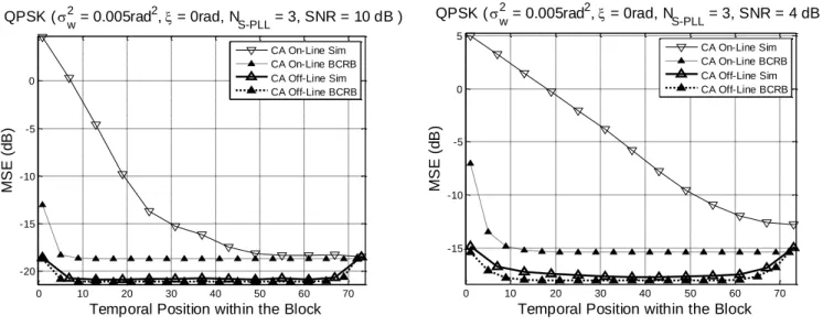
conventional Gray mapper. After passing through the phase uncertain channel, blocks of L complex-valued symbols (BPSK, QAM) are finally received by the carrier recovery block such as depicted by Fig. 2. MSEs are evaluated over 105 Monte Carlo trials and the corresponding curves are noted “Sim” in the following figures. Moreover, we also use the following notations: “On-Line” means that the MSE is the conventional forward estimation without any backward estimation, and “Off-Line” means that the MSE is measured after NS-PLL3 forward and backward iterations.

0 10 20 30 40 50 60 70 -20 -15 -10 -5 0

Temporal Position within the Block

M S E ( d B ) QPSK (  w 2 _{= 0.005rad}2_{,  = 0rad, N} S-PLL = 3, SNR = 10 dB ) CA On-Line Sim CA On-Line BCRB CA Off-Line Sim CA Off-Line BCRB 0 10 20 30 40 50 60 70 -15 -10 -5 0 5

Temporal Position within the Block

M S E ( d B ) QPSK (  w 2 _{= 0.005rad}2_{,  = 0rad, N} S-PLL = 3, SNR = 4 dB ) CA On-Line Sim CA On-Line BCRB CA Off-Line Sim CA Off-Line BCRB

Fig. 3 MSE curves for the various positions in the block at two different SNRs.

Figure 3 compares different on-line and off-line MSE performance to Bayesian CRBs [30],[31] for a block of L=72 coded QPSK modulated signals. For the on-line scenario, the MSE lowers down towards the on-line BCRB as more and more samples are processed. However, the off-line estimator performance is always better than the on-line estimator performance. This is because the off-line estimator is able to reach the off-line BCRB which is a few dBs

under the on-line BCRB. As also illustrated by figure 4 and figure 5, DA and NDA curves would lead to similar conclusions, the non-coded performance being itself inferior to the coded-scheme, especially at low SNR.

We now display various results where L864for QPSK and L1152for 16QAM. Instead of looking at the different

positions for some given SNRs, we now display the phase estimation error curves as function of the SNR in the central position of the block.

0 5 10 15 20 25 30 -30 -25 -20 -15 -10 -5 SNR (dB) M S E ( d B ) QPSK (  w 2 = 0.005rad2,  = 0rad, N S-PLL = 3 ) CA Sim (On-Line) CA BCRB (On-Line) DA Sim (On-Line) DA BCRB (On-Line) CA Sim (Off-Line) CA BCRB (Off-Line) DA Sim (Off-Line) DA BCRB (Off-Line)

Fig. 4 QPSK performance in the center position versus SNR with no linear drift

When the linear drift 0, both the on-line and off-line algorithms can reach the corresponding BCRBs and work

very well in a large SNR range (see figure 4). At high SNR, each current observation is reliable enough to estimate the current phase shift and there is neither a gain with a block proceeding nor any phase synchronization problem. At more realistic average to low SNRs, as it was already depicted on figure 3 for any position, the off–line approach allows to benefit from a gain of several dBs. The reason for this result is that one observation is not sufficient to correctly estimate the symbols while a block of more observations should be used to improve the estimation performance. At low SNR, when the code is not efficient anymore, the CA curves leave the DA curves. The superiority of the off-line bound is even enhanced when there is a linear drift as illustrated on the following figure 5.

5 10 15 20 25 30 -35 -30 -25 -20 -15 -10 -5 SNR (dB) M S E ( d B ) QPSK (  w 2 = 0.0005rad2,  = 0.01rad, N S-PLL = 3 ) NDA Sim (On-Line) NDA HCRB (On-Line) CA Sim (On-Line) CA HCRB (On-Line) NDA Sim (Off-Line) NDA HCRB (Off-Line) CA Sim (Off-Line) CA HCRB (Off-Line)

Fig. 5 QPSK performance in the center position versus SNR, with a linear drift 0

The conclusions for figure 5 with a linear drift are similar to figure 4 but we can specify three more facts. First, the MSEs must now be compared to Hybrid CRBs because there is a (large) deterministic linear drift  and all the curves are poorer than the curves obtained with no linear drift. Second, for SNRs spanning from mid-range to low range, the on-line scheme is not able to reach anymore its HCRB; this comes from the classical fact that a traditional PLL becomes biased for larger and larger linear drift (see for instance [17]). Third, the CA MSEs leave their asymptote regime at lower SNRs than the NDA curves and this might be useful for terminals forced to work at low SNRs.

5 10 15 20 25 -34 -32 -30 -28 -26 -24 -22 -20 -18 -16 SNR (dB) M S E ( d B )

16QAM ( _w2 = 0.0004rad2,  = 0rad, N_S-PLL = 3 )

NDA Sim (On-Line) CA Sim (On-Line) DA Sim (On-Line) DA BCRB (Off-Line) NDA Sim (Off-Line) CA Sim (Off-Line) DA Sim (Off-Line) DA BCRB (Off-Line) 5 10 15 20 25 -34 -32 -30 -28 -26 -24 -22 -20 -18 -16 -14 SNR (dB) M S E ( d B )

16QAM ( _w2 = 0.0002rad2,  = 0.003rad, N_S-PLL = 3 )

NDA Sim (On-Line) CA Sim (On-Line) DA Sim (On-Line) DA HCRB (On-Line) NDA Sim (Off-Line) CA Sim (Off-Line) DA Sim (Off-Line) DA HCRB (Off-Line)

Similar results, are obtained for a 16QAM modulated signal at larger SNRs with (right part of Figure. 6) or without (left part of Figure. 6) a linear drift. The advantage of using an off-line scenario is predominant for all the synchronizing schemes. As the SNR becomes lower and lower, the NDA curves leave the CRBs first, before the CA curves and finally the DA curves. In this SNR range, the error control coding becomes critical to improve the estimation performance; however, once again, the main result from this figure is that for most of the SNRs, though it has a lower complexity, the off-line NDA SPLL is generally able to give better (or similar) results than the on-line CA PLL. -4 -3 -2 -1 0 1 2 3 4 5 10-5 10-4 10-3 10-2 10-1 SNR (dB) B E R QPSK (  w 2 _{= 0.0009rad}2_{,  = 0rad, N} S-PLL = 3 ) NDA On-Line CA On-Line NDA Off-Line CA Off-Line AWGN

Fig. 7 Influence of the phase recovery on BER curves

Finally, figure 7 represents the BER curves for various scenarios (off-line/on-line, NDA/CA) for a QPSK modulated signal. Clearly, the off-line scenario is superior to its on-line counterpart; also, the CA scheme allows to gain up to 1 dB compared to the NDA scheme for the off-line scenario. We note with interest that a CA off-line scheme is able to work at about 0.5 dB from the perfect phase recovery scheme (AWGN channel).

VIII. CONCLUSION

In this paper, we derived a near-MAP phase estimator for generally coded and modulated symbols which is made out of two first order PLLs possibly aided by some decoded a posteriori information. The MSE performance of the S-PLL

provides a gain of several decibels when compared to a classical forward on-line algorithm; it can reach the Cramer-Rao bounds of interest over a wide range of SNRs and we proved the asymptotic convergence. Moreover, it is to be high-lighted that low-complexity NCA off-line schemes often give better results than the classical turbo recovery (CA on-line PLLs). Smoothing loops do not suffer from a poor transient behavior and are robust against frequency offsets. They are easy to implement, especially compared to CA (such as turbo) phase recovery schemes and thus, they could be very useful in practice.

REFERENCES

[1] G. Colavolpe, G. Ferrari, and R. Raheli, “Noncoherent iterative (Turbo) decoding,” IEEE Trans. Commun., vol. 48, pp. 1488–1498, Sept. 2000.

[2] G. Colavolpe, A. Barbieri, and G. Caire, “Algorithms for iterative decoding in the presence of strong phase noise,” IEEE J. Select. Areas Commun., vol. 23, pp. 1748–1757, Sept. 2005.

[3] J. Dauwels and H.-A. Loeliger, “Joint decoding and phase estimation: An exercise in factor graphs,” in Proc. IEEE ISIT’03, p. 231, Yokohama, Japan, June 29-July 4, 2003.

[4] J. Dauwels and H.-A. Loeliger, “Phase estimation by message passing,” in Proc. IEEE ICC’04, pp. 523–527, New York, USA, June 20-24, 2004.

[5] M. Nissila and S. Pasupathy, “Adaptive Iterative Detectors for Phase-Uncertain Channels via Variational Bounding,” IEEE Trans. on Commun., vol. 57, pp.716-725, Mar. 2009.

[6] D. D. Lin and T. J. Lim, “The variational inference approach to joint data detection and phase noise estimation in OFDM,” IEEE Trans. on Signal Processing, vol. 55, pp. 1862-1874, May 2007.

[7] P.O. Amblard, J.M. Brossier, and E. Moisan, “Phase tracking: what do we gain from optimality? Particle filtering versus phase-locked loops,” Signal Processing, vol. 83, pp. 151-167, Oct. 2003.

[8] M. J. Nissila, S. Pasupathy, and A. Mammela, “An EM approach to carrier phase recovery in AWGN channel,” in Proc. IEEE ICC’01, pp. 2199–2203, Helsinki, Finland, June 11-15, 2001.

[9] N. Noels, C. Herzet, A. Dejonghe, V. Lottici, H. Steendam,M. Moeneclaey, M. Luise, and L. Vandendorpe, “Turbo synchronization: an EM algorithm interpretation,” in Proc. IEEE ICC’03, pp. 2933–2937, Anchorage, Alaska, May 11-15, 2003.

[10] F. M. Gardner, Phaselock Techniques, 3rd ed., Wiley-Interscience, 2005.

[11] L. Zhang and A. Burr, “Iterative Carrier Phase Recovery suited for Turbo-Coded systems,” IEEE Trans. on Wireless Commun., vol. 3, pp. 2267-2276, Nov. 2004.

[12] N. Noels, H. Steendam and M. Moeneclaey, "Performance Analysis of ML-Based Feedback Carrier Phase Synchronizers for Coded Signals," IEEE Transactions on Signal Processing, vol. 55, pp. 1129-1136, March 2007. [13] N. Noels, H. Steendam, M. Moeneclaey, "Effectiveness Study of Code-Aided and Non-Code-Aided ML-Based

Feedback Phase Synchronizers," in Proc. IEEE ICC'06, Istanbul, Turkey, June 11-15, 2006.

[14] S. Bay, C. Herzet, J.P. Barbot, J. M. Brossier, and B. Geller, "Analytic and Asymptotic Analysis of Bayesian Cramer–Rao Bound for Dynamical Phase Offset Estimation," IEEE Transactions on Signal Processing, vol. 56, pp. 61-70, Jan. 2008.

[15] S. Bay, B. Geller, A. Renaux, J.P. Barbot, and J.M. Brossier, “On the Hybrid Cramer-Rao bound and its application to dynamical phase estimation,” IEEE Signal Processing Letters, vol. 15, pp. 453-456, 2008.

[16] J. Yang and B. Geller, “Bayesian and Hybrid Cramer-Rao Bounds for the Carrier Recovery under Dynamic Phase Uncertain Channels,” IEEE Trans. on Signal Processing,pp. 667-680, Feb. 2011.

[17] J. Yang and B. Geller, “Near Optimum Low Complexity Smoothing Loops for Dynamical Phase Estimation - Application to BPSK Modulated Signals,” IEEE Trans. on Signal Processing, pp. 3704-3711, Sept. 2009. [18] B. Geller, J. P. Barbot, J.M. Brossier, C. Vanstraceele, Procédé d’estimation de la phase et du gain de données

d’observation transmises sur un canal de transmission. French patent Fr2005002301. International extension WO2006032768 on the 30th March 2006.

[19] J. Yang, B. Geller, C. Herzet, and J.M. Brossier, “Smoothing PLLs for QAM Dynamical Phase Estimation,” in Proc. IEEE Inter. Conf. on Commun. 2009, ICC'09, Dresden, 14-18 June 2009.

[20] N. Noels, M. Moeneclaey, F. Simoens, and D. Delaruelle, “A Low-Complexity Iterative Phase Noise Tracker for coded Bit-Interleaved CPM Signals in AWGN,” IEEE Trans. on Signal Processing, vol.59, pp. 4271-4284, Sept.

[21] F. Lehmann, “A Gaussian Sum Approach to Blind Carrier Phase Estimation and Data Detection in Turbo Coded Transmissions,” IEEE Trans. on Communication, vol. 57, pp. 2619-2632, Sept. 2009.

[22] J. A. McNeill, “Jitter in ring oscillators,” Ph.D. dissertation, Boston University, 1994.

[23] A. Demir, A. Mehrotra, and J. Roychowdhury, “Phase noise in oscillators: a unifying theory and numerical methods for characterization,” IEEE Trans. Circuits Syst. I, vol. 47, pp. 655–674, May 2000.

[24] ETSI EN 302 307 “Digital Video Broadcasting (DVB); Second Generation Framing Structure, Channel Coding and modulation systems for Broadcasting, Interactive Services, News Gathering and other broadband satellite applications,” June 2004.

[25] S. M. Kay, Fundamentals of Statistical Signal Processing: Estimation Theory. Upper Saddle River, NJ, USA: Prentice-Hall, Inc., 1993.

[26] L. Bahl, J. Cocke, F. Jelinek, and J. Raviv, “Optimal Decoding of Linear Codes for Minimizing Symbol Error Rate,” IEEE Trans. on Info. Theory, vol. IT-20(2), pp. 284-287, Mar, 1974.

[27] J. Pearl, “Reverend Bayes on inference engines: A distributed hierarchical approach,” in Proc. American Association of Artificial Intelligence National Conference on AI, pp.133-136, Pittsburgh, PA. 1982.

[28] J. Pearl, Probabilistic Reasoning in Intelligent Systems: Networks of Plausible Inference (Revised Second Printing), San Francisco, CA: Morgan Kaufmann, 1988.

[29] A. Cochran, Carrier Phase Synchronization by Reverse Playback. International patent PCT US 1997/022067, WO1998024210 on the 4th Jun. 1998.

[30] J. Yang, B. Geller, and A. Wei, “Bayesian and Hybrid Cramer-Rao Bounds for QAM Dynamical Phase Estimation,” in Proc. IEEE Signal Processing, ICASSP'09, Taipei, 19-24 April 2009.

[31] J. Yang, B. Geller, and A. Wei, “Approximate Expressions for Cramer-Rao Bounds of Code Aided QAM Dynamical Phase Estimation,” in Proc. IEEE Inter. Conf. on Commun. 2009, ICC'09, Dresden, 14-18 June 2009. [32] D. Divsalar and F. Pollara, “Turbo codes for PCS applications,” in Proc. ICC’95, pp. 54-59, Seattle, WA, June

APPENDIX

DERIVATIONS OF ERROR TERMS

The first derivative of lnp y θ

 

, can be calculated from (11)-(12) ; for 1 m L_{, we thus get} ln  ,

m p    y θ  



 



       







 



   





  2 1 1 1 1 2 2 2 1 1, 1 1 ln | , , ln , | , , | , , | , , K K L l l l v l v v l m m m m m m L m m m v m l l l v l v v l l m m L l l l v l v v l p y s s p p p y s s p y s s p p y s s p                                           _    _   _              _            

 

 



c c c y θ c c c c c c c  





     





 





     



 



1 1 2 2 2 2 2 1 1 1 1 2 2 2 2 1 2 2 | , , | , , 2 | , | , , | , , ln | , , 2 | , K K m m m L m m m v m l l l v l v v l m m m m m m m v m v v m m m v m v m m p y s s p y s s p p p y s s p p y s s p                             _{   }                  _  _   _          _{ }    



 



c c c c y θ c y c c θ c c c y θ    



 



 



 



1 1 2 2 2 1 1 1 2 2 2 2 1 1 2 1 , | , ln | , , 2 | , ln | , , 2 Pr | , , , K K m m v m m m v m v m m m m m m m v m m m m v v m p y s s p y s s           _{ }                           _{ }             





c c y θ c y θ c c c y θ (45) where       , | , Pr | , , | , v v p p       c c y θ c c y θ

y θ is the normalized a posteriori probability (APP) of the codeword cv.

Assuming that we do not have any priori information about 1 (i.e.

 1 1 ln 0 p   

 ), similarly to obtaining (46), we can

easily obtain the first derivatives for m1 and mL

  2 _{ }



 



  1 1 1 1 2 1 2 1 1 1 ln | , , ln , Pr | , , K v v v y s s p                    



 c r θ c c y θ (47)   2 _{ }



 



  1 2 1 ln | , , ln , Pr | , , K L L L v L L L v v L L y s s p                     



 c r θ c c y θ , (48)

where the exact expression ln  l| l, , l l

p y   s

 

 can be obtained from (49)

  2 Im





ln | , , _{y s e} jl

p y   s  