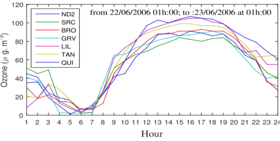
Ozone measurements monitoring using data-based approach
Texte intégral
Figure


Documents relatifs
The corrosion fatigue analysis mainly considered the effect of variable amplitude loading (pressure fluctuation) on small weld defects. The Miners rule and Paris
The results obtained in the conducted experiments with models based on various distribution laws of the requests flow intensity and the criteria used are used as input information
‚ A low level DSL allows a security expert to extend a list of predefined access control patterns defined within our DSL tool, and to create a custom transformation module in
L’archive ouverte pluridisciplinaire HAL, est destinée au dépôt et à la diffusion de documents scientifiques de niveau recherche, publiés ou non, émanant des
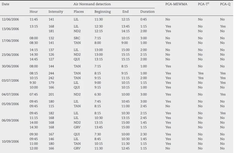
Process monitoring using multivariate statistical process control (MSPC) has attracted large industries types due to its practical importance and application.. In this paper, a
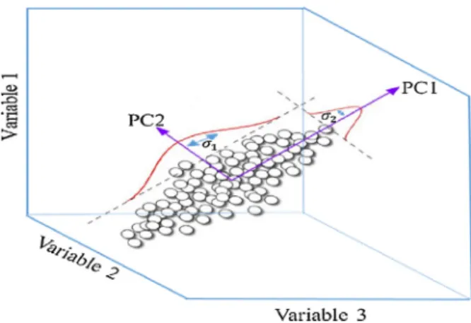
I It can be chosen such that the components with variance λ α greater than the mean variance (by variable) are kept. In normalized PCA, the mean variance is 1. This is the Kaiser
The dashed curve represents the standard (relativistic) PWIA calculation, the solid curve is the (non-relativistic) Faddeev calculation with FSI effects only, and the dot-dashed
Plusieurs noyaux de l’atlas Colin 27 ont été regroupés pour définir une entité du Template comme les groupes nucléaires thalamiques.. La majorité des noyaux étaient
