Any correspondence concerning this service should be sent to the repository administrator: [email protected]
This is an author’s version published in: http://oatao.univ-toulouse.fr/22413
To cite this version: Ravat, Franck and Song, Jiefu A
Unified Approach to Multisource Data Analyses. (2018)
Fundamenta Informaticae, 162 (4). 311-359. ISSN 1875-8681
Official URL
DOI : https://doi.org/10.3233/FI-2018-1727 Open Archive Toulouse Archive Ouverte
OATAO is an open access repository that collects the work of Toulouse researchers and makes it freely available over the web where possible
DOI 10.3233/FI-2018-1700
A
Unified Approach to Multisource Data Analyses
Franck Ravat Jiefu Song∗IRIT - Universit´e Toulouse I Capitole
2 Rue du Doyen Gabriel Marty F-31042 Toulouse Cedex 09, France [email protected], [email protected]
Abstract. Classically, Data Warehouses (DWs) supports business analyses on data coming from the inside of an organization. Nevertheless, Lined Open Data (LOD) might sensibly complete these business analyses by providing complementary perspectives during a decision-making pro-cess. In this paper, we propose a conceptual modeling solution, named Unified Cube, which blends together multidimensional data from DWs and LOD datasets without materializing them in a stationary repository. We complete the conceptual modeling with an implementation frame-work which manages the relations between a Unified Cube and multiple data sources at both schema and instance levels. We also propose an analysis processing process which queries dif-ferent sources in a transparent way to decision-makers. The practical value of our proposal is illustrated through real-world data and benchmarks.
Keywords: Data Warehouse, Linked Open Data, Conceptual Modeling, Multisource analyses, Experimental Assessments
1.
Introduction
Well-informed and effective decision-making relies on appropriate data for business analyses. Data are considered appropriate if they include enough information to provide an overall perspective to decision-makers. To obtain as many appropriate data as possible, decision-makers must have access to the company’s business data at any time. Since the 1990s, Business Intelligence (BI) has been ∗Address for correspondence: IRIT - Universit´e Toulouse I Capitole, 2 Rue du Doyen Gabriel Marty F-31042 Toulouse
providing methods, techniques and tools to collect, extract and analyze business data stored in a Data Warehouse(DW) [9]. However, an overall perspective during decision-making requires not only busi-ness data from inside a company but also other data from outside a company. In today’s constantly evolving business context, one promising approach consists of blending web data with warehoused data [32]. The concept of BI 2.0 is introduced to envision a new generation of BI enhanced by web-based content [39].
Among various web-based content, Linked Open Data (LOD)1 provide a set of inter-connected and machine-readable data to enhance business analyses on a web scale [45]. Since data are produced and updated at a high speed nowadays, materializing all data (e.g., warehoused data and LOD) related to analyses in one stationary repository can hardly be synchronized with changes in data sources. It is necessary to unify data from various sources without integrating all data into a stationary repository. To support up-to-date decision-making, business dashboards must be created in an on-demand manner. Such dashboards should include all appropriate data required by decision-makers.
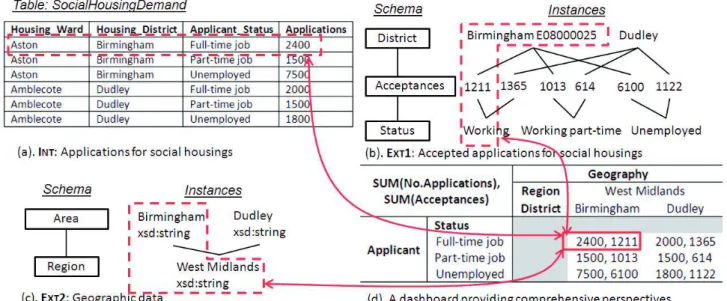
Case Study. In a government organization managing social housings, internal data are periodi-cally extracted, transformed and loaded in a DW. As shown in figure 1(a), the DW describes number of applications (i.e. Applications) according to two analysis axes: one about the geographical location of social housings (i.e. Housing Ward and Housing District) and the other related to applicant’s profile (i.e. Applicant Status). This DW only gives a partial view on the demand for social housings. To support effective decision-making, additional information should be included in analyses. Therefore, a decision-maker browses in a second dataset, named LOD1, to obtain complementary views on so-cial housing allocation. Published by the UK Department for Communities and Local Government2, LOD1 describes the accepted applications for social housing (i.e. acceptance) according to district
Figure 1: An extract of data in a DW and two LOD datasets 1http://linkeddata.org
and status (cf. figure 1(b)). LOD1 follows a multidimensional structure expressed in RDF Data Cube Vocabulary(QB)3. The QB format only allows including one granularity in each analysis axis. The decision-maker needs new analysis possibilities to aggregate data based on multiple granularities. To discover more geographical granularities, the decision-maker looks into another dataset named LOD2. This dataset is managed by the Office for National Statistics of the UK4; it associates several areas (including districts) with one corresponding region (cf. figure 1(c)). Both LOD1 and LOD2 are real-world LOD which can be accessed through querying endpoints56.
The above-mentioned warehoused data and LOD share some similar multidimensional features, as they are organized according to analysis subjects and analysis axes. However, analyzing data scattered in several sources is difficult without a unified data representation. During analyses, decision-makers must search for useful information in several sources. The efficiency of such analyses is low, since different sources may follow different schemas and contain different data instances. Facing these issues, the decision-maker needs a business-oriented view unifying data from both the DW and the LOD datasets. She/he makes the following requests regarding the view:
• An analysis subject should include all related numeric indicators from different sources, even though these indicators cannot be aggregated according to the same analytical granularities. To support real-time analyses, numeric indicators (e.g. Applications from the DW, Acceptances from the LOD1 dataset) and their descriptive attributes (e.g. Housing Ward, Housing District and Applicant Status from the DW, District and Status from the LOD1 dataset) at different analytical granularities should be queried on-the-fly from sources;
• Analytical granularities related to the same analysis axis should be grouped together. For in-stance, the Housing Ward and Housing District granularities from the DW, the District granu-larity from the LOD1 dataset, the Area and Region granularities from the LOD2 dataset should be merged into one analysis axis;
• Attributes describing the same analytical granularity should be grouped together. The correl-ative relationships between instances of these attributes should be managed. For instance, the attribute Housing District from the DW, the attribute District from the LOD1 dataset and the attribute Area from the LOD2 dataset should be all included in one analytical granularity related to districts. Correlative instances ”Birmingham” from the DW, ”Birmingham E08000025” from the LOD1 dataset and ”Birmingham xsd:string” from the LOD2 dataset should be associated together, since they both refer to the same district;
• Summarizable analytical granularities should be indicated for each numeric indicator. For in-stance, only the measure Applications from the DW can be aggregated according the Ward analytical granularity. The other measure Acceptances from the LOD1 dataset is only summa-rizable starting from the district analytical granularity on the geographical analysis axis. 3http://www.w3.org/TR/vocab-data-cube
4https://www.ons.gov.uk/
5http://opendatacommunities.org/sparql 6http://statistics.data.gov.uk/sparql
Contribution. Our aim is to make full use of as much information as possible to support effective and well-informed decisions. To this end, we propose a unified view of data from both DWs and LOD datasets. At the schema level, the unified view should include in a single schema all information about an analysis subject described by all available analysis axes as well as all granularities (coming from multiple sources). At the instance level, the unified view should not materialize data that can be directly queried from the source. Nevertheless, it should manage the correlation relations between related attribute instances referring to the same real-world entity. With the help of the unified view, a decision-maker can easily obtain an overall perspective of an analysis subject. In the previous example, a unified view would enable decision-makers to analyze on-the-fly the number of applications and acceptancesaccording to applicant’s status and district as well as region (cf. figure 1(d)).
In this paper, we describe a generic modeling solution, named Unified Cube, which provides a business-oriented view unifying both warehoused data and LOD. Section 2 presents different ap-proaches to unifying data from DWs and LOD datasets. Section 3 describes the conceptual modeling and graphical notation of Unified Cubes. Section 4 presents an implementation framework for Unified Cubes. Section 5 shows how analyses are carried out on a Unified Cube in a user-friendly manner. Section 6 illustrates the feasibility and the efficiency of our proposal through some experimental as-sessments.
2.
Related work
Disparate data silos from different sources make decision-making difficult and tedious [43]. To pro-vide decision-makers with an overall perspective during business analyses, an effective data integration strategy is needed. In accordance with our research context, we focus on work related to the integra-tion of multidimensional data from DWs and LOD datasets. We classify existing researches into three categories.
The first category is named ETL-based. With the arrival of LOD, the BI community intuitively treated LOD as external data sources that should be integrated in a DW through ETL processes [15, 29, 36]. The obtained multidimensional DW is used as a centralized repository of LOD [38, 6]. Decision-makers can use classical DW analysis tools to analyze LOD stored in such DWs. However, the existing ETL techniques are inclined to populate a DW with LOD rather than updating existing LOD in a DW. No effective technique is proposed to guarantee the freshness of warehoused LOD presented to decision-makers during analyses. One promising avenue is to extend on-demand ETL processes [4] to fit for the integration of LOD in a DW at right time during business analyses. Otherwise, current ETL-based approaches are not suitable in today’s highly dynamic context where large amounts of data are constantly published and updated; they collide with the distributed nature and the high volatility of LOD [24, 17].
The second category is named semantic web modeling. Since multidimensional models have been proven successful in supporting complex business analyses [35], the LOD community introduces new modeling vocabularies to semantically describe the multidimensionality of LOD through RDF triples. Among the proposed modeling vocabularies, the RDF Data Cube Vocabulary7(QB) is the current W3C 7http://www.w3.org/TR/vocab-data-cube
standard to publish multidimensional statistical data. The authors of [26] carry out multidimensional analyses over QB datasets. It is worth noticing that a QB dimension is a non-hierarchical concept. Due to this limit, the authors fail to support analyses involving multiple hierarchies within a dimen-sion. To overcome this drawback, extensions of the QB vocabulary are needed to model a complete multidimensional schema. In [17], the authors propose the QB4OLAP vocabulary which adds more multidimensional characteristics to QB, like multiple analytical granularities within multiple aggrega-tion paths and the specificaaggrega-tion of the aggregaaggrega-tion funcaggrega-tions associated with a measure. The authors of [37] present a multidimensional data model by blending together QB, SKOS8and RDFs9 vocabu-laries. They also show how multidimensional analysis operations are translated into SPARQL queries based on the proposed data model. However, all semantic web modeling vocabularies are based on RDF formats which are primarily intended for machine consumption [37] and thus cannot be easily used by decision-makers. Even though the authors of [17, 37] provide conceptual models underlying semantic web modeling vocabularies, a user-oriented graphical notation is still missing to facilitate decision-makers’ tasks of exploring RDF-like data schemas. Moreover, the work [26, 37] deals only with one LOD dataset. To handle data other than LOD, the work [17] uses mappings (i.e. R2RML) to populate a QB4OLAP dataset with warehoused data. Yet, no information is provided about if any of the above-mentioned work can integrate both warehoused data and LOD in one single dataset. With-out solutions to these problems, current semantic web modeling approaches is not suitable for the unification of heterogeneous data in one user-oriented schema.
The third category is named unified modeling. It aims at providing generic data modeling solutions to (i) provide an overall representation of multisource data and (ii) manage relationships between mul-tisource data. The authors of [1] envision a multidimensional model in which an internal database is gradually extended by fusing with external data, especially with data from the Web. The authors of [2] outline a new multidimensional model to support user-guided data discovery and acquisition of both internal warehoused data and external Web data. The unified modeling is a promising solution which allows blending data from multiple sources together. However, the work [1, 2] only describes gen-eral principles and research orientations. The authors of [28] propose IGOLAP vocabulary allowing representing multisource data according to a multidimensional structure. However, the compatibility of the work [28] is limited to LOD datasets. To deal with warehoused data, the authors suggest (i) transforming them into LOD formats through a mapping language proposed in [25] and (ii) loading large amounts of transformed data into a IGOLAP dataset. Consequently, the work [28] faces the same problems of the ETL-based work. Moreover, the feasibility of unifying multisource data in a IGO-LAP dataset is only discussed without being experimentally assessed. It remains unknown how the complete unification process is instantiated and how heterogeneous instances from different sources are managed in a IGOLAP schema.
In this paper, we propose a generic multidimensional model which provides a unified view of both warehoused data and relevant multidimensional LOD. We denote our solution as data unification to differ from classical data integration solutions. Our data unification solution should break away from full integration of data into a stationary repository. It should keep a unified view over internal data (warehoused data) and external data (multidimensional LOD) without materializing all data. Based 8https://www.w3.org/TR/skos-reference/
on the unified modeling, we propose a complete unification process including the implementation of a unified view and the processing of on-the-fly analyses on multisource data through a unified view.
3.
Conceptual modeling of Unified Cubes
Unifying internal warehoused data and external LOD is not a straight forward task [33]. On one hand, DW and LOD communities do not share the same modeling paradigms. No existing data model allows blending multisource data without materializing them in a stationary repository. On the other hand, related data instances are scattered in different schemas. Existing modeling solutions without materialization do not allow managing the relations between heterogeneous instances from different sources. Facing these problems, we propose a new conceptual modeling solution, named Unified Cube, which is generic enough to unify (i) business data which are stored in multidimensional DWs from inside a company and (ii) multidimensional LOD which are stored in sources from outside a company. The Unified Cube modeling extends the classical multidimensional modeling to provide a single, comprehensive representation of multisource data. In the following section, we describe the Unified Cube model through an abstract representation. This representation is oriented towards designers who define a conceptual schema based on multisource data. A graphical notation of the abstract representation is proposed to facilitate the exploration of a Unified Cube by decision-makers.
3.1.
Analysis subject: fact
Classically, a fact models an analysis subject. The fact is composed of a set of numeric indicators called measures. To support real-time analyses, the Unified Cube modeling extends the concept of measure by allowing on-the-fly extraction of measure values.
Definition 3.1. A fact is characterized by a name and a set of measures. It is denoted as F = {nF; MF
} where:
• nF is the fact’s name;
• MF = {m1; . . . ; mp} is a finite set of numeric indicators called measures. Each measure me (me ∈ MF) is a pairhnme, Emei, where nme is the name of a measure and Eme is an extraction formuladefined through a query algebra (e.g., relational algebra and SPARQL algebra10). The values of the measuremeare denoted as val(me).
Remark. Extraction formulae enable on-the-fly querying of measures’ values during analyses. The algebraic representation of extraction formula makes sure its compatibility with specific imple-mentation environments of data source. Note that although the SPARQL algebra is not yet a W3C standard, it has already been integrated within several RDF querying framework. Each algebraic SPARQL expression is translated into one SPARQL query which is generic enough to work with all types of LOD datasets. Table 1 shows the algebraic form of commonly used SPARQL queries. 10https://www.w3.org/2001/sw/DataAccess/rq23/rq24-algebra.html
Table 1: SPARQL queries and their algebraic representation. Query 1 SELECT * WHERE{ ?s ?p ?o} Algebraic representation (BGP (TRIPLE ?s ?p ?o)) Query 2 SELECT ?s ?p WHERE{?s ?p ?o} Algebraic representation
(PROJECT(?s ?p) (BGP (TRIPLE ?s ?p ?o))) Query 3
SELECT ?o1 ?o2 WHERE{?s ?p ?o1. FILTER (?o1< 5)
OPTIONAL{?s ?p2 ?o2 . FILTER ( ?o2> 10 ) }}
Algebraic representation
(PROJECT(?o1 ?o2) (FILTER (< ?o1 5) (LEFTJOIN(BGP (TRIPLE ?s ?p ?o1)) (BGP (TRIPLE ?s ?p2 ?o2)) (> ?o2 10))))
Query 4 SELECT ?s (COUNT(?o) as ?nb) WHERE{?s ?p ?o} GROUP BY ?s HAVING (COUNT(?o)> 10) Algebraic representation (PROJECT(?s ?nb) (FILTER (> ?.0 10) (EXTEND((?nb ?.0)) (GROUP (?s) ((?.0 (COUNT ?o))) (BGP (TRIPLE ?s ?p ?o))))))
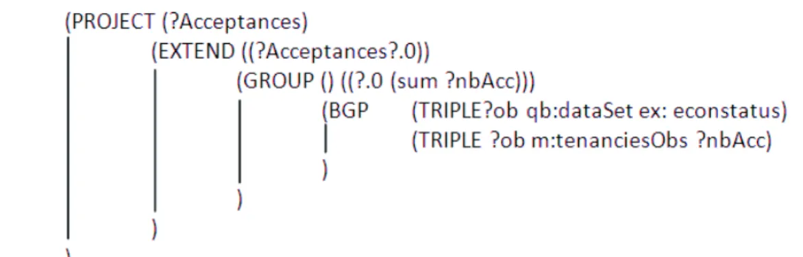
Example. The fact named Social Housings contains two measures, namely mAcceptances and mApplications. The measure mApplications has an extraction formula expressed in relational algebra, such as: EmApplications = Fsum(SocialHousingDemand.Applications). The extraction formula of the measuremAcceptancesis defined upon SPARQL algebra, such as:
3.2.
Analysis axis: dimension
The concept of dimension in a Unified Cube follows the classical definition. A dimension may include a single or multiple analytical granularities. If several analytical granularities are defined, we can find one or several aggregation paths (also known as hierarchies).
Definition 3.2. A dimension corresponds to a one-dimensional space regrouping the analytical gran-ularities related to one analysis axis. A dimension is denoted asDi={nDi; LDi; 4Di}, where:
• nDi is the dimensions name;
• LDi={l1; . . . ; lk} is a set of analytical granularities called levels;
• 4Di is a binary relation which associates a child level la (la ∈ LDi) with a parent level lb (lb∈ LDi), such asla 4Di lb.
Example. We identify a dimension named Geography which groups all analytical granularities re-lated to social housing’s location. It includes three levels, such asLGeography = {lGeo.W ard; lGeo.District; lGeo.Region}. The binary relation 4Geography reveals the aggregation paths (i.e., hierarchies) such as lGeo.W ard4Geography lGeo.District4Geography lGeo.Region.
Our definition of dimension is generic enough to model a non-hierarchical dimension as well. A non-hierarchical dimension (e.g. DQB) has only one level (e.g., LQB = {l1}) including all the attributes of the dimension.
Two hierarchies from different sources do not always share a common lowest analytical granular-ity. Therefore, we remove the constraint of unique root level (i.e.,∃=1lp ∈ LDi, ∀lq ∈ LDi : lp 4Di lq11) in the definition of a dimension. Without this constraint, a dimension may start at any level. This is an important property of a dimension regrouping levels from multiple sources, since measures from one source may only be analyzed according to a subset of levels coming from the same source. We define a sub-dimension as a part of dimension along which a measure can be summarized.
Definition 3.3. A sub-dimension of Di, denotedDi\ls = { nDi\ls; LDi\ls; 4Di}, corresponds to the part of the dimensionDistarting with the level ls, where :
• nDi\ls is the name of the sub-dimension;
• LDi\ls is the subset of levels,LDi\ls ⊆ LDi, ∀li∈ LDi\ls, ls 4Di l i; • 4Di is the same binary relation of the one on the dimensionDi.
Example. A sub-dimension of the geographical dimension isDGeography\lGeo.Districtnamed Geography-Districtwith LDGeography\lGeo.District={lGeo.District; lGeo.Region}, which represents the subpart of the dimensionDGeography that the measuremAcceptancesfrom the LOD1 dataset is linked to.
11∃
3.3.
Analytical granularity: level
Classically, a level indicates a distinct analytical granularity described by a set of attributes from the same data source. In the context of Unified Cubes, the classical definition of level needs to be extended to group together attributes from different sources. Specifically, a level should manage a set of attributes by (i) indicating how attribute instances can be extracted from data sources and (ii) representing correlation relationships between related attribute instances from different sources. Definition 3.4. A level represents an analytical granularity of a dimension. A level is denoted as ld = {nld; Ald; Cld}, where:
• nld is the levels name; • Ald = {a
1; . . . ; ae} is a finite set of attributes. Each attribute ax(ax ∈ Ald) is a pairhnax, Eaxi, wherenax is the name of the attribute and Eax is an extraction formula indicating how instances ofax can be extracted from the corresponding source. The domain of an attribute is denoted as dom(ax);
• Cld : dom(ax) −→ dom(ay)(ax ∈ Ald, ay ∈ Ald \ ax) is a symmetric transitive correlative mapping. It connects instances of the attributeaxwith equivalent instances of the attributeay, i.e. for an attribute instanceix∈ dom(ax), there exists at most one instance iy ∈ dom(ay), such as Cld(ix) = iy.
Example. The level lEconomic.Statuson the dimensionDApplicant contains a finite set of attributes AlEconomic.Status = {aStatus; aApplicant Status}. To associate each attribute with its instances in data sources, two extraction formulae are defined within this level: EaApplicant Status =
πApplicant Status(SocialHousingDemand) is linked to the attribute aApplicant Status from the DW, while the attributeaStatus has the following extraction formula:
The correlative mapping ClEconomic.Status associates the instances of the attribute aStatus with its equivalent instances of the attributeaApplicant Status, such as:
ClEconomic.Status : {{Working} −→ {Full-time Job}; {Working part-time} −→ {Part-time job}; {Unemployed} −→ {Unemployed}}.
3.4.
Unified Cube
In a Unified Cube, a fact and a dimension respectively include measures and levels from multiple sources. Each measure can be aggregated according to the set of levels from the same source. For each measure, decision-makers need to easily distinguish summarizable levels from non-summarizable lev-els. To do so, we propose the level-measure mapping which is flexible enough to associate each measure with a set of dimensions starting from any level.
Definition 3.5. A Unified Cube is a n-dimensional finite space describing a fact with some dimen-sions. It is denoted asU C = {F ; D; LM}, where:
• F is a fact containing a set of measures; • D={D1; . . . ; Dn} is a finite set of dimensions;
• ∀me ∈ MF, LM: 2L1\lp×...Ln\lq −→ me is a level-measure mapping which associates a sub-set of summarizable analytical granularities (i.e., levels) with a measure me, such as ∀i ∈ [1..n], Li\ls(ls ∈ Li) corresponds to a subset of levels on the dimension Di(Di ∈ D) which starts from the level ls.
We propose a graphical notation for Unified Cubes by extending the star schema notation proposed in [21]. The modifications are as follows:
• A fact is represented by a rectangle. The fact name is situated within the rectangle on top; • A measure is circled by a rectangle;
• A dimension is enclosed by a rectangle. The name is placed above a dimension; • Each level is represented by a circle with all its descriptive attributes lying below; • A binary relation is represented by an arrow from a child level to a parent level;
• A level-measure mapping is represented by a line between a measure and a dimension starting from any level. In order to simplify the notation, the level-measure mapping is drawn between a measure and its lowest summarizable levels within corresponding dimensions.
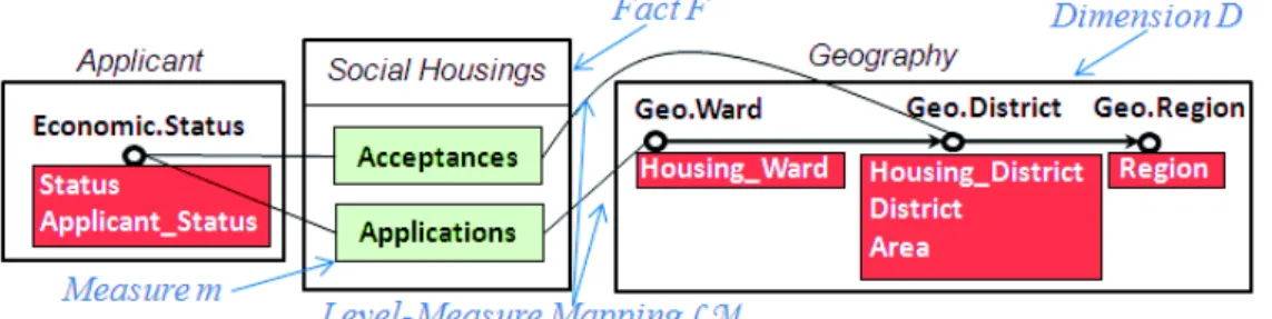
Example. The Unified Cube of our case study contains two dimensionsD = {DApplicant, DGeography}. The two measures of the fact named Social Housings are associated with their summarizable lev-els, i.e., LM:{ {LApplicant; LGeography\lGeo.District}−→ {mAcceptances}; {LApplicant; LGeography} −→ {mApplications} }. The complete graphical notation of this Unified Cube is shown in figure 3.
3.5.
Main contributions of Unified Cube modeling
To the best of our knowledge, Unified Cube is the first model that allows unifying appropriate data for decision-making from both DWs and LOD datasets without materializing all data in a stationary repository. By including business-oriented concepts and a graphical notation, a Unified Cube can sup-port analyses on multiple data sources in a user-friendly way without requiring specialized knowledge on logical or physical data modeling. The Unified Cube modeling breaks through three obstacles in the multidimensional modeling field: (i) warehoused data and LOD can be queried on-the-fly during analyses through instance-finding mappings (i.e. extraction formulae of measures and attributes), (ii) a measure can be linked to a dimension starting from any level through intra-aggregate mappings (i.e. level-measure mapping LM), and (iii) attribute instances from one source are linked with equivalent instances of attribute from another source through inter-instance mappings (i.e. correlative mappings Cld). The powerful Unified Cube modeling is further coupled with a user-friendly graphical nota-tion, so that non-expert users can easily explore by themselves the overall schema of multisource data during analyses.
4.
Implementation of Unified Cubes
A conceptual Unified Cube provides a generic representation unifying data which are physically stored in different sources. Once defined by a schema designer, a Unified Cube needs to be implemented before being used to support analyses on multisource data. To do so, we provide a framework which automates the implementation of Unified Cubes. Two modules are identified within the framework, namely schema and instance. The schema module aims at managing the overall structure of a Unified Cube (cf. section 4.1), while the instance module serves as an integrated repository of correlative attribute instances from heterogeneous sources (cf. section 4.2).
4.1.
Schema module
The schema module manages the multidimensional representation of a Unified Cube. It serves as an interface between business-oriented concepts in a Unified Cube and referents in data sources. To do so, we propose a metamodel which offers a uniform way to access different data sources through concepts in a Unified Cube. In this section, we firstly describe the components of the metamodel. Then, we propose an algorithm to automatically instantiate the metamodel.
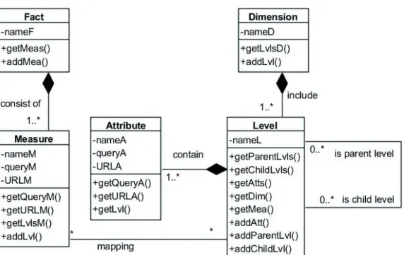
In the metamodel, concepts such as fact, measure, dimension, level and attribute are modeled through classes. Composition relationships are used to associate a containing class (e.g., fact) with a contained class (e.g., measures). Binary relations between parent and child levels are represented by a recursive association connected to the Level class. Level-measure mappings are managed by the association between classes named Measure and Level. It is worth noticing that extraction formulae of measures and attributes are translated into executable queries (i.e., queryM and queryA). A querying endpoint is associated with each measure and each attribute, so that data instances can be extracted on-the-fly during analyses. The class diagram of the metamodel is shown in figure 4.
We complete the proposed metamodel with an instantiation process (cf. algorithm 1). The goal is to automatically instantiate classes and associations of the metamodel based on a conceptual Unified
Figure 4: Class diagram of the metamodel for Unified Cubes
Cube. First, the algorithm instantiates the dimension class and associates each dimension instance (Dmeta
i ) with related attributes instances (ametax ) organized according to child (lmetae ) and parent (lmetaf ) level instances (cf. lines 1 - 16). Then, the algorithm creates a fact instance (Fmeta) and links it with a set of measure instances (mmeta
g ) (cf. lines 17 - 22). At last, the algorithm instantiates associations between a measure instance (mmetag ) and its summarizable level instances (Lr\lh × . . . × Lt\lk) (cf. lines 23 - 26). The output of the instantiation process is an instantiated metamodel which manages the overall structure of a Unified Cube.
Specifically, each Unified Cube dimension is used to instantiate a Dimension class (cf. lines 1 and 2). For each level on the Unified Cube dimension, a Level class is instantiated and associated with the corresponding Dimension class (cf. lines 3 - 5). The extraction formula of an attribute in the Unified Cube is transformed into an equivalent algebraic operation before being translated into an executable query. An Attribute class is instantiated with a name, a query and a query endpoint. It is then associated with the corresponding level (cf. lines 6 - 11). Binary relations within a dimension are used to instantiate the association between a child level instance and a parent level instance (cf. lines 13 - 15). A Fact class is instantiated (cf. lines 17). An executable query is generated for each measure based on the extraction formula. With the measure’s name, translated query as well as query endpoint, a Measure class is instantiated and associated with the fact (cf. lines 18 - 22). The level-measure mappings in the Unified Cube are used to instantiate the association between a measure instance and a set of level instances (cf. lines 23 - 26). Note that the operations used in the algorithm can be found in the metamodel in figure 4.
Example. We apply the algorithm to the Unified Cube of our case study (cf. figure 3). The instan-tiated metamodel contains (i) one instance of Fact (ii) two instances of Measure, (iii) two instances of
Algorithm 1: Metamodel Instantiation input : A Unified Cube ={F; D ; LM } output: An instantiated metamodel for eachDi ∈ D do
Instantiate the Dimension class: Dmeta
i = newDimension(nDi); for each ld ∈ LDi do
Instantiate the Level class: lmetad = newLevel(nld); Dimeta.addLvl(lmetad );
for each ax ∈ Ald do
Translate the extraction formulaEax into a queryQax; Get the attribute’s query endpointU RLax;
Instantiate the Attribute class:ametax = newAttribute(nax; Qax; U RLax); ametax .addLvl(lmetad ) ;
end end
for each le 4Di lf do
lmetae .addP arentLvl(lmetaf ), lmetaf .addChildLvl(lmetae ); end
end
Instantiate the Fact class: Fmeta = newF act(nF) ; for eachmg ∈ MF do
Translate the extraction formulaEmg into a queryQmg; Get the measure’s query endpointU RLmg;
Instantiate the Measure class: mmeta
g = newM easure(nmg; Qmg; U RLmg); Fmeta.addM ea(mmetag );
Find levels Lr\lh × . . . × Lt\lk associated withmg through level-measure mappingsLM, such as Lr\l h × . . . × L t \lk ⊆ L 1 × . . . × Ln,LM: Lr\lh × . . . × Lt\l k −→ mg; for each level lh ∈ Lr\lh × . . . × Lt\lk do
mmeta
g .addLvl(lmetah ); end
end
Dimension, (iv) four instances of Level with two associations implementing binary relations and seven associations implementing level-measure mappings and (v) seven instances of Attribute.
In figure 5, a snapshot of the instantiated metamodel is presented in the form of an object diagram. For the sake of readability, the snapshot only includes some components of the Unified Cube of the case study. In the snapshot, the Geography dimension includes the level Geo.District. This level contains three attributes from the DW and the two LOD datasets, namely District, Housing District and Area. The measure named Acceptances of the fact named Social Housings is mapped to the summarizable level Geo.District through level-measure mappings.
Figure 5: Snapshot of instantiated metamodel
4.2.
Instance module
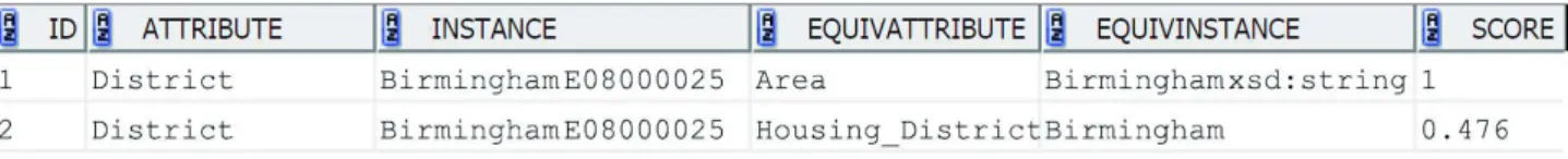
In a Unified Cube, equivalent attribute instances from different sources are associated together by cor-relative mappings (cf. section 3.3). Due to different understandings of the same real-world concepts, equivalent attribute instances may take heterogeneous forms in different data sources. It is necessary to bridge the differences among multiple data sources at the instance level. To do so, we propose a table of correspondences which manages correlative mappings between related attribute instances. Definition 4.1. A table of correspondences links up pairs of correlative attribute instances by annotat-ing each pair with a confidence score. Its schema is denoted asT = {id; nax; iax; nay; iay; scorexy}, where:
• id is an identifier;
• naxis the name of the attributeax;
• iax is an instance of the attributeax,iax ∈ dom(ax);
• iay is an instance of the attributeay,iay ∈ dom(ay);
• scorexy is a normalized confidence score betweeniax andiay,scorexy ∈ [0, 1].
Populating a table of correspondences requires identifying correlative instances from different sources. In some cases, correlative mappings are already semantically represented between sources. For instance, it is common to find in a LOD dataset that the OWL propertyowl:sameAs is used to associate an instance with an equivalent instance in another LOD dataset. A table of correspondences is populated by directly following such existing correlative mappings.
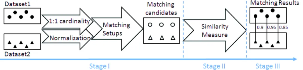
In other cases, there exists no correlative mapping between two sources (e.g. between a DW and a LOD dataset). We rely on techniques of instance matching to identify correlative instances between two datasets. Instance matching belongs to the field of entity resolution [12, 5]. Existing entity res-olution processes are designed for matching instances from sources of the same type. Classically, problems of matching instances from sources of different types are handled in a simplistic way by transforming heterogeneous sources into a common format and then following a matching process designed for homogeneous sources. However, as more and more data are involved in matching nowa-days, it is not efficient to carry out matching with a transformation stage. The matching should be performed directly between different sources, regardless if the sources belong to the same type or not. To do so, we propose a process based on techniques which are generic enough to enable direct matching of instances from heterogeneous sources. As shown in figure 6, the process starts with a stage which generates matching candidates directly from raw data. The second stage consists of calculating the similarity between matching candidates. The final stage determines the best matches between the two sets of instances.
Figure 6: Process of matching between two sets of instances from different sources
Specifically, during the first stage, we apply some processing techniques to prepare attribute in-stances for the matching. First, we fix the matching cardinality to 1:1 (i.e. injective mapping), which assumes one instance in a source can be matched with only one instance in the other source. Second, we normalize descriptive information of instances by eliminating stylistic differences due to capi-talization, punctuation, and non-Latin characters. Third, we propose several solutions to set up the matching candidates in string form.
• A straightforward setup consists of concatenating all descriptive information into one long string. We denote this setup as Concatenated. The opposite setup is to compare individually descriptive information of the same kind [27]. We denote this setup as Separated.
• Some descriptive information may contain useless parts, e.g., name spaces such as the prefix eg:12. We propose a setup named Optimized which removes useless parts to keep only informa-tion related to matching [10]. The opposite setup is denoted Unprocessed, as it takes descriptive information ”As-Is” without any modification.
Remark. In the case where each instance is described by one unique string, the matching is carried out directly with the unique description of an instance without concatenation.
During the second stage, we rely on string similarity measures to calculate a confidence score between 0 and 1 for each pair of matching candidates. String similarity measures are widely used as syntax-based matching technique in the field of entity resolution [19], for instance, record linkage between warehoused data [7] and instance matching between LOD [9]. We identify sixteen widely-used string similarity measures in the scientific literature. We carry out some experimental assessments to find out the most efficient string similarity measures. Based on the results, we identify three string similarity measures, namely N Grams Distance [40], Levenshtein [44], and Smith Waterman [30], which are generic and efficient enough to fit for various matching tasks. Details about our experimental assessments will be presented in section 6.
Remark. Matching based on string similarity measures is often reinforced by some auxiliary techniques. One of the most widely used auxiliary techniques is semantic-based. It relies on formally described semantics to perform deductive matching methods. However, in nowadays open, evolving world, different sources usually adopt different methods to describe the semantics. Matching two sources with well-defined semantics through semantic-based techniques is already hard enough, e.g. ontology and instance matching tracks of Ontology Alignment Evaluation Initiative13, not to mention difficulties in matching data from semantic-light sources, such as DWs. A DW’s semantics are not rich enough, since they are defined during the design phase and not explicitly represented after implemen-tation [18]. An intermediate ontology is generally used to provide additional semantics of warehoused data [20]. Building an intermediate ontology usually requires the intervention of domain experts and thus is hardly automated. Moreover, the slightest error in an intermediate ontology can introduce hidden bias in matching. Therefore, semantic-based techniques using an intermediate ontology are neither generic nor efficient enough to be applied to instance matching in a Unified Cube.
During the third stage, we determine the best matches by finding 1:1 matching between two sets of instances. We apply the stable-marriage algorithm [22] to identify mutually accepted matching between two datasets. The algorithm repeats the following steps until all instances in two datasets are matched: letD1 andD2be two datasets, (i) an unmatched instance inD1establishes a mapping with the most similar instance inD2if no previous mapping is broken between them and (ii) an instance in D2accepts a mapping fromD1and breaks an existing mapping (if any) when the new mapping comes from a more similar instance in D1. A set of best matches between two data sources is produced. Then, the best matches are used to populate the table of correspondences.
Example. In the Unified Cube of our case study, the level lGeo.District includes three attributes from different sources. Correlative instances are identified in the following ways:
12eg:¡http://www.example.org/¿ 13http://oaei.ontologymatching.org/
Figure 7: Identifying equivalent attribute instances within the level lGeo.District
• the attributes named District and Area come from the LOD1 and LOD2 datasets respectively. In the LOD1 dataset, each district is linked to an equivalent district in the LOD2 dataset through the OWL property owl:sameAs (cf. figure 7). By referring to the links between LOD datasets, 243 pairs of districts from the LOD1 dataset and the LOD2 dataset are associated together with a perfect confidence score (i.e. score = 1);
• Housing District’s instances from the DW share similar description with instances of Area from the LOD1 dataset. Yet, there is no existing correlative mapping between the DW and the LOD1 dataset. We apply our proposed instance matching process to identify correlative instances of the attributes Housing District and Area.
A snapshot of the obtained table of correspondences is shown in figure 8.
Figure 8: A snapshot of the table of correspondences
The advantage of our implementation framework is twofold. On one hand, instances are not ma-terialized and can be queried on-the-fly. In this way, the data freshness is guaranteed during analyses. On the other hand, data from different sources can be analyzed in a unified way owing to the table of correspondences. The cost of maintaining a table of correspondences is quite low, as attribute instances only represent 1% to 6% of a multidimensional dataset’s size [42].
5.
Analysis processing of Unified Cubes
Our proposed implementation framework enables interactions between a Unified Cube and multiple data sources at both schema and instance levels. Based on the framework, we propose an analysis processing process enabling decision-making on multiple sources in a user-friendly way.
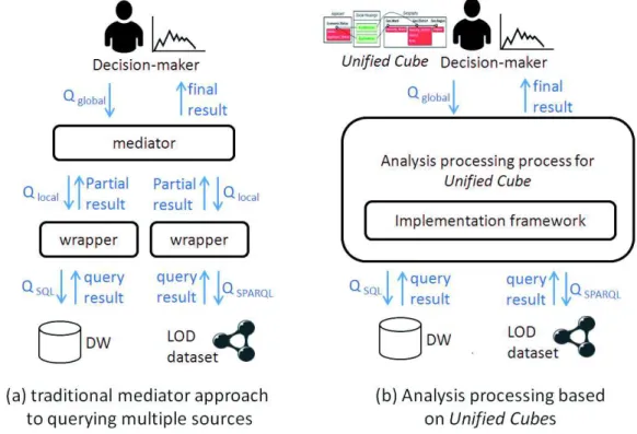
Processing analyses on multiple sources has been studied by classical mediator approaches. As shown in figure 9(a), in the mediator-based approach, a query posed over a global schema (i.e.Qglobal) is transformed into local queries (i.e. Qlocal) by a mediator. A wrapper translates a local query into an executable query in one source. Query results are transformed into a common form (e.g., relational data) to generate partial results of analysis. All partial results are then combined together to form a final analysis result [3].
Figure 9: Mediator-based approach versus analysis processing process for Unified Cube Comparing to classical mediator-based approaches, our proposed analysis processing process is saved from the intermediate steps in wrappers: executable queries are directly generated based on a global query posed over a Unified Cube, while a final analysis result is directly built from extracted multisource data. Specifically, at the beginning of an analysis, a decision-maker explores a Unified Cubeand expresses a global query by choosing a set of attributes and measures related to the analysis. The analysis processing process automatically generates executable queries in multiple sources by us-ing the extraction formulae stored in the implementation framework. After the execution of queries, data from several query results are automatically blended together by referring to the correlative re-lations provided by the implementation framework. At the end of an analysis, the decision-maker receives one unique analysis result including data from multiple sources.
In this section, we first describe how queries are automatically generated for an analysis (cf. sec-tion 5.1). Then, we present how one analysis result is generated based on data extracted from different sources (cf. section 5.2). At last, we illustrate the feasibility of our proposal through a prototype analysis framework (cf. section 5.3).
5.1.
Queries generation
With the help of a Unified Cube, a decision-maker can express an analysis need by choosing a set of measures and attributes. To facilitate decision-makers tasks, we propose a process whose goal is to extract data related to an analysis from multiple sources (cf. algorithm 2). This is done through the generation of queries in each data source involved in an analysis.
First, among the chosen attributes, the algorithm finds a subset of attributes (AM) that are directly related to chosen measures (M ) (cf. lines 1 - 23). Then, for each chosen measure (me), the algorithm generates a query by combining its extraction formula and those of the related attributes (Ame) (cf. lines 24 - 30). At last, if there are some chosen attributes (A\ AM) that are not directly related to any chosen measure, their extraction formulae are added in the set of generated queries (cf. lines 31 -35). The output of the algorithm is a set of queries extracting data related to an analysis from multiple sources. The abstract notation of Unified Cubes and operations involved in the algorithm are described in previous sections 3 and 4.1 respectively.
Specifically, in a Unified Cube, each measure is summarizable with regard to a set of levels. The set of summarizable levels may differ from one measure to another, while not every measure can be calculated according to every level (e.g. figure 3). If an analysis mistakenly involves a measure and attributes within non-summarizable levels, the algorithm displays a warning message and breaks the execution (cf. lines 7 - 8). Otherwise, the algorithm classifies measures and attributes by data source. Specifically, for each measureme, the algorithm finds a list of attributes from the same sources (i.e. Ame in line 4). Such attributes may (i) be an attribute ax chosen by decision-makers (cf. lines 10 and 11), (ii) correspond to an attribute within the same level of ax (i.e. ay at lines 14 and 15) and (iii) come from the set of attributes within the highest level linked tome (i.e. ay bis at lines 17 and 18). Extraction formulae of a measure and its attributes are then grouped together (cf. lines 24 - 26). As some analyses involve multiple levels, grouping predicates have to be added in generated queries (cf. line 27). During the execution, the algorithm picks out attributes linked to a chosen measure (i.e. AM in lines 1 and 23). For the other attributes (i.e. A\ AM in line 32), the algorithm directly adds their extraction formulae in the set of queries (i.e. Q ). Each query in the output result includes measures and attributes from a single source.
To better explain how the algorithm works, we show some examples of analysis based on the Unified Cubeof our case study (cf. figure 3).
The first analysis includes a measure and an attribute from different sources. The algorithm firstly finds the set of levels linked to the measuremAcceptences(cf. line 3, LmAcceptences =
LGeography\lGeo.District ∪ LApplicant. Then it retrieves the chosen attribute’s level (cf. lines 6, laHousing W ard). By comparing laHousing W ard with LmAcceptences, the algorithm finds that the chosen measure is not linked to the level of the chosen attributes (cf. line 7, laHousing W ard ∈ L/ mAcceptences). It displays a warning message and stops executing (cf. line 8). No query is generated for the first
Algorithm 2: Automatic Query Generation
input : A set of measures M ; a set of attributes A output: A set of generated queries Q ={q1; . . . qn } Create an empty set of attributes AM, AM = ∅; for eachme ∈ M do
Get all levels linked tome: Lme = me.getLvlsM (); Create an empty list of attributes Ame, Ame = ∅ ; for eachax ∈ A do
Get the level ofax: lax = ax.getLvl(); if lax ∈ L/ me then
Impossible analysis, break the execution and display a warning message; else
ifax.getU RLA() = mx.getU RLM () then Add the attributeaxin the list Ame; else
Get the set of attributes on the level lax: Alax = lax.getAtts(); if∃ay ∈ Alax such asay.getU RLA() = me.getU RLM () then
Add the attributeayin the list Ame; else
Find an attributeayBis, such asayBis.getLvl() ∈ lax.getChildLvls() ∧ ∄az ∈ ayBis.getLvl().getP arentLvl().getAtts(), az.getU RLA() = me.getU RLM () ;
Add the attributeayBisin the list Ame; end
end end end
AM ←− AMSAme;
Get the query of the measureme:qme = me.getQueryM (); for eachap ∈ Ame do
Addap.getQueryA() in qme;
Addapin the grouping predicates inqme ; end Addqme in Q; if A\ AM 6= ∅ then for eachax∈ A \ AM do Addak.getQueryA() in Q end end end
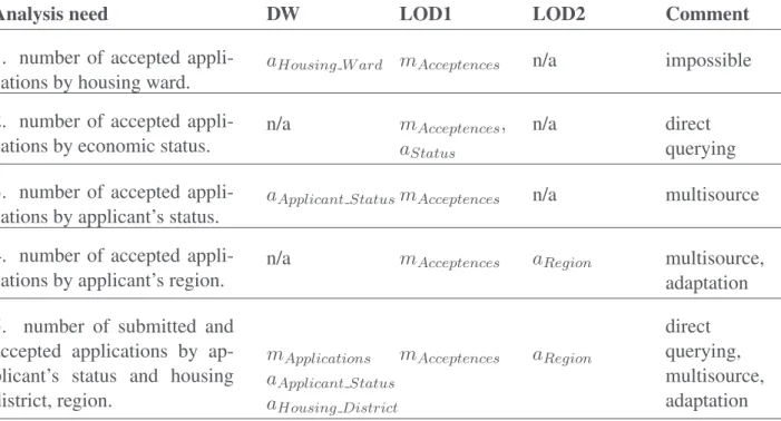
Table 2: Analysis needs with corresponding measures and attributes
Analysis need DW LOD1 LOD2 Comment
1. number of accepted appli-cations by housing ward.
aHousing W ard mAcceptences n/a impossible 2. number of accepted
appli-cations by economic status.
n/a mAcceptences,
aStatus
n/a direct
querying 3. number of accepted
appli-cations by applicant’s status.
aApplicant StatusmAcceptences n/a multisource 4. number of accepted
appli-cations by applicant’s region.
n/a mAcceptences aRegion multisource, adaptation 5. number of submitted and
accepted applications by ap-plicant’s status and housing district, region. mApplications aApplicant Status aHousing District mAcceptences aRegion direct querying, multisource, adaptation
analysis. Through the first example, we can see our proposed algorithm is reliable enough to detect analysis needs that are not supported.
The second analysis corresponds to a classical involving only one data source. In this case, measures and attributes can be directly queried from the source. Specifically, after verifying that mAcceptencesandaStatus come from the same source, the algorithm combines their extraction formu-lae together (cf. lines 10 and 11). The generated query in appendix A shows a Unified Cube also supports analyses involving one single data source.
The third analysis calculates a measure according to an attribute from a different source. The algo-rithm first retrieves all attributes within the same level ofaApplicant Status(cf. line 13, AlaApplicant Statue) ={aApplicant Status, aStatus}). An attribute aStatusis found in the same source of measuremAcceptences (cf. line 14,aStatus ∈ AlaApplicant Statue,aStatus.getURLA()=mAcceptences.getURLM()). The extrac-tion formulae ofmAcceptencesandaStatusare combined together in the same way of the second anal-ysis (cf. line 15). The algorithm finds the relative complement of AlaApplicant Statuein chosen attribute set A is not empty (cf. line 31, A\AlaApplicant Statue={aStatus}). The extraction formula of aStatus is added in the set of generated queries (cf. line 33). Appendix B shows the two generated queries of the third analysis.
The fourth analysis involves two different sources. No attribute within the level of aRegion be-longs to the source ofmAcceptances (cf. lines 13 and 14, ∄ay ∈ laRegion.getAtts(), ay.getURLA() 6= mAcceptances.getULLM()). Adaptations are needed to generate executable queries for each source. To do so, the algorithm finds aDistrict which belongs to a lower level of laRegion and the high-est level available in the source of mAcceptances (cf. line 17, laDistrict ∈ laRegion.getChildLvls()
∧∀az ∈ laDistrict.getParentLvl().getAtts(), az.getURLA() 6= mAcceptances.getURLM()). The first query is generated by combining together the extraction formulae of aDistrict and mAcceptances (cf. line 18), while the second query is generated by directly using the extraction formula ofaRegion. Both queries are present in appendix C.
The fifth analysis unifies measures and attributes from three different sources. The extraction formulae of mApplications, aApplicant Status and aHousingDistrict are directly combined together to generate the first query, since they come from the same DW (cf. lines 10 and 11). Then, the algorithm finds attributes aStatus and aDistrict from the LOD1 dataset (cf. lines 13, 14 and 17). The second query is generated by referring to the extraction formulae ofmAcceptances, aStatus andaDistrict (cf. lines 15 and 18). The third query refers directly to the extraction formula ofaRegion(cf. lines 31 - 34). The last analysis covers all previously discussed scenarios: from a single source to multiple sources with and without adaptation. Three generated queries are shown in appendix D.
5.2.
Analysis result generation
After the execution of generated queries, several query results are returned from different sources. It is difficult for decision-makers to obtain an overall perspective from different query results containing data of different types. It is necessary to provide one unified result including all data related to the analysis. To do so, we propose a generic modeling solution of query result and analysis result which can be considered as a set of attribute instances possibly linked to a set of measure values.
Definition 5.1. A result is denoted asRi= {VRi; IRi; fRi}, where:
• VRi = ∅ ∨ {val(m1), . . . , val(mf)} is an empty set or a set of measure values;
• IRi = {IDi, . . . , IDp} is a non-empty set of attribute instances organized according to dimen-sions. ∀IDx ∈ IRi, IDxrefers to the attribute instances on the dimensionDx;
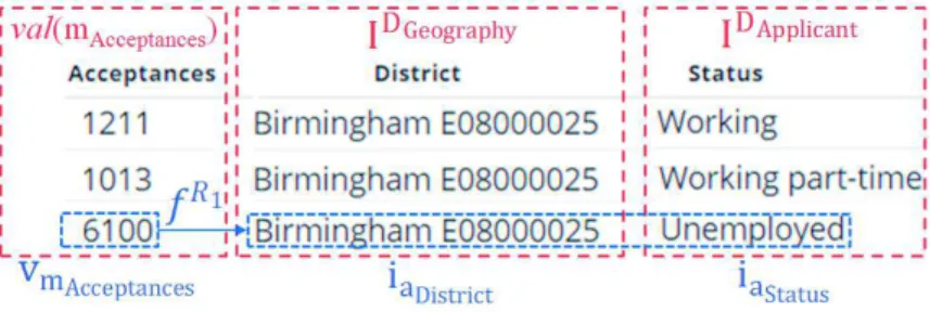
• fRi : VRi −→ IRi is a function associating each n-tuple of measure values {vm1, . . . , vmf } to one n-tuple of attribute instances {ia1, . . . , iae }, where ∀vmx ∈ {vm1, . . . , vmf}, vmx is a value of the measure mx (i.e. vmx ∈ val(mx) ) and ∀iay ∈ {ia1, . . . , iae}, iay is an instance of the attribute ay (i.e. iay ∈ dom(ay)). In particular, when a result contains only attribute instances without any measure value (i.e. VRi = ∅), fRi is an empty function.
Example. Figure 10 shows the number of accepted applications for social housing by district and economic status (i.e. the result of the second generated query in appendix D).
Based on the generic modeling of result, we propose a process whose goal is to generate an overall result at the end of an analysis (cf. algorithm 3). This is done by blending together data from one or several query results. When one single query result is obtained (|R| = 1), it is considered as the final analysis result (cf. lines 1 and 2). When several query results are produced, they are combined together by reference to the related instances (T= {T1, ..., Tk}) stored in the table of correspondences (cf. lines 3 - 22). In the following, we provide more details about how multiple query results are fused together to form one analysis result at the output of the algorithm.
Algorithm 3: Automatic generation of Analysis Result
input : A set of chosen attributes A ; a set of query results returned from sources R ={R1, . . . , Rn}.
output: A single analysis resultRAnalysis if|R|=1 then
RAnalysis= R ; else
Find a query result Rx, such asRx∈ R ∧ VRx 6= ∅; Create a temporary resultRtemp, setRtemp←− Rx;
Get the set of tuples T ={T1, . . . , Tk} in the table of correspondences; for each resultRi∈ R ∧ Ri6= Rxdo
for each set of attribute instance IDx on the dimensionDxin resultRi, IDx ⊆ IRi do Find the set of attribute instances IDxbis on the same dimensionDxin IRtemp; for each pair of instancesiap andiaq, such asiap ∈ IDx ∧iaq ∈ IDx
bis
∧∃id ∈ N, ∃score ∈ R, there exists a tuple in the table of correspondances, such as{id, ap.getN ameA(), iap, aq.getN ameA(), iaq, score} ∈ T do
Associateiap withiaq inRtemp; if VRi 6= ∅ then
Create fRtemp between VRi ∪ VRtemp and IDx ∪ IDx bis; else
Create fRtemp between VRtemp and IDx ∪ IDxbis; end
end end end
AggregateRtempaccording to the chosen attributes A; RAnalysis ←− Rtemp;
end
Specifically, the algorithm first creates a temporary result Rtemp based on one query result con-taining some measure values (cf. lines 4 and 5). Then, each n-tuple of attribute instances inRtemp is
associated with a related n-tuple in query resultRi. This is done by referring to tuples in the table of correspondences (cf. lines 6 - 11). Meanwhile, ifRi includes some measures, related measure values fromRtempandRiare grouped together and linked to the corresponding attribute instances inRtemp (cf. lines 12 and 13). If no measure is involved inRi, only measure values fromRtempare associated with related attribute instances (cf. line 15). At last, a single analysis result is generated by aggregating the measures inRtemp according to the attributes specified by a decision-maker (cf. lines 20 and 21). Note that the abstract notation in algorithm 3 follows the conceptual Unified Cube modeling presented in sections 3, while the operations correspond to those in the metamodel described in section 4.1.
Example. To explain the execution of the algorithm 3, we illustrate how the analysis result is gen-erated for the most complex analysis (the fifth analysis) in table 2. Remember that three queries were generated for this analysis: the first queryR1aggregates the sum ofmApplications byaHousing District and aApplicant Status from the DW; the second query R2 aggregates the sum of mAcceptances by aDistrict andaStatus from the LOD1 dataset; the third queryR3 associates each district (i.e. aArea) with its region (i.e. aRegion) from the LOD2 dataset without any measure.
After the execution of all generated queries, the algorithm 3 receives three results from different sources. It first creates a temporary result Rtemp based on the query result R1 from the DW (cf. figure 11(1)). Then, attribute instances fromRtempare grouped with those fromR2(cf. figure 11(2)). During this step, attribute instances involved in correlative mappings are grouped together by referring to the table of correspondences (cf. lines 6 - 11 in algorithm 3). Next, measure values fromRtempare associated with related ones fromR2(cf. figure 11(3)).
Figure 11: Combining query results from the DW and the LOD1 dataset
Query resultR3does not contain any measure. It provides a complementary level of the geograph-ical dimension inRtemp. To mergeR3withRtemp, the algorithm refers to the table of correspondences
to associate instances ofaDistrict with those ofaArea. The instances of aRegion are merged into new Rtempalong with corresponding areas (cf. figure 12).
Figure 12: CombiningRtempwith query result from the LOD2 dataset
The final analysis result is generated by aggregating measures according to attributes chosen by a decision-maker. In our example, the attributesaApplicant Status,aHousing DistrictandaRegionconsists of the chosen attributes of the analysis (cf. table 2), the algorithm automatically generates a query aggregating the temporary result according toaApplicant Status,aHousing DistrictandaRegion(cf. lines 19 and 20 in algorithm 3). The final analysis result is shown in figure 13.
Figure 13: Analysis result about number of submitted and accepted applications by applicant’s status and housing district, region
The advantages of our proposed support process are twofold. First, our proposed decision-support process always provides up-to-date data to decision-makers. Warehoused data and LOD are queried on-the-fly during analyses without materializing them in a stationary repository. Second, our proposed decision-support process facilitates decision-makers analysis tasks. An analysis result
based on data from various sources is automatically created in an on-demand manner. In this way, the distribution of data throughout multiple sources, the different schemas of various sources, and the complex querying languages with specific syntax are all hidden from end users by our proposed decision-support process.
5.3.
Multisource analysis framework
To enable analyses on multiple sources in a user-friendly manner, we develop a multisource analysis framework which present only business-oriented concepts to decision-makers during analyses. The overall architecture of the multisource analysis framework is shown in figure 14.
Figure 14: Architecture of the multisource analysis framework
Specifically, a Unified Cube is implemented at both the schema and the instance levels by schema manager and instance manager respectively. The schema manager deals with concepts related to the unified view of multiple data sources. It is made up of (i) a metamodel implemented in the Or-acle DBMS and (ii) a Java program instantiating the metamodel. The instance manager deals with correlative attribute instances from different sources. The Oracle DBMS hosts a relational table of correspondences in the instance manager. A Java program implements our instance matching process and populates the relational table of correspondences. Note that a Unified Cube can be built upon any source which provides a querying endpoint (e.g., an internal DW fully controlled by an organization, an external DW hosted by a business partner, an online LOD dataset, . . . ). Moreover, it is possible to populate the table of correspondences on-the-fly and keep it in memory without materialization. How-ever, to reduce analysis runtime, we choose to populate the table of correspondences prior to querying and materialize it in a relational DBMS.
The analysis processing methods are implemented through two Java programs. They allow (i) generating queries to extract data from multiple sources and (ii) integrating extracted data into one analysis result. Both Java programs are included in the analysis processing manager. Note that queries discussed in section 5.1 (cf. appendixes) and analysis results presented in section 5.2 are automatically generated by the analysis processing manager of our multisource analysis framework.
We develop a graphical interface by extending the ones of our previously proposed analysis tools [35, 34]. The interface aims at facilitating interactions between a decision-maker and the multisource
analysis framework. As shown in figure 15, a decision-maker can express an analysis need by choosing measures and attributes within related levels through the graphical notation of Unified Cubes (cf. upper part of the graphical interface). At the end of an analysis, a decision-maker can visualize an analysis result in tabular and graphic forms (cf. lower part of the graphical interface).
Figure 15: Graphical interface of the multisource analysis framework
Our proposed analysis framework supports a user-friendly decision-making process in our analysis framework. As shown in figure 14, a decision-maker starts an analysis by exploring a Unified Cube in graphical notation through an interface (cf. arrow 1). She/he clicks on measures and attributes related to her/his analysis needs. The interface sends the chosen measures and attributes to the schema manager (cf. arrow 2). The latter looks up in the metamodel to find extraction formulae and query endpoints of the chosen measures and attributes (cf. arrow 3). Next, the analysis processing manager generates a set of queries and sends them to the corresponding query endpoints of different sources. Each query includes measures and attributes from one source (cf. arrows 4). After queries execution, the analysis processing manager receives data extracted from different sources (cf. arrows 5). It then refers to the correlative relationships in the instance manager to associate equivalent attribute instances together among extracted data (cf. arrow 6). One analysis result is generated by the analysis processing managerbased on the chosen measures and attributes (cf. arrow 7). At last, the interface provides the decision-maker with a dashboard representing the analysis result in tabular and graphic forms (cf. arrow 8). In this way, decision-makers only interact with some business-oriented concepts during analyses. The analysis processing is completely hidden from decision-makers.
6.
Experimental assessments
To enable analyses on data from multiple sources, one key step consists of unifying data extracted from different sources together to form one unique analysis result. This unification is based on the table of correspondences which is populated through an instance matching process (cf. figure 6). By exclusively using string similarity measures, our proposed matching process is generic enough to identify correlative instances without formally described data semantics. To study the feasibility and efficiency of our proposed matching process, we carry out some experimental assessments.
In this section, we first describe the inputs of our experimental assessments composed of two data collections and sixteen string similarity measures (cf. section 6.1). Second, we present the results of our experimental assessments. We also discuss the influences of four matching setups and different features of data collections on matching efficacy and efficiency (cf. section 6.2). Third, based on the experimental results, we propose some generic guidelines for efficient use of string similarity measures to match correlative instances in a Unified Cube (cf. section 6.3). At last, we validate our proposed guidelines by using benchmarks of Ontology Alignment Evaluation Initiative14(cf. section 6.4).
6.1.
Input
During our experimental assessments, we use two collections of real-world data. Each collection covers a specific domain and has distinctive features.
The first collection is named GeoData. It contains geographic data in the RDF format published by the UK Department for Communities and Local Government (CLG)15. The CLG provides multidimen-sional LOD datasets related to social housing, taxation of local governments, etc. Most CLG datasets contain a geographic dimension composed of one level named District. The geographic dimension can be completed by adding more levels such as County and Region published by the Office for National Statistics (ONS)16. To do so, each District from the CLG dataset is associated with a corresponding District from the ONS dataset through the propertyowl:sameAs. These correspondences are used as baselines, i.e. a set of actual mappings between instances from two datasets. The objective is to match 237 non-metropolitan districts from the CLG dataset with 280 non-metropolitan and metropoli-tan districts from the ONS dataset. The percentage of mismatches is(280 − 237)/237 = 18.14%. The CLG dataset includes 25 079 RDF triples, while the ONS dataset contains only 4256 RDF triplet. Descriptive information about districts, such as name and type, is relatively short. The average string length is 24.6 characters including data type descriptors and name spaces.
The second collection is named DBLP. It contains bibliographic data related to scientific publica-tions provided by DBLP (e.g. conference papers, journal articles, etc.). Two different implementapublica-tions of the bibliographic data are managed by the European Network of Excellence ReSIST17 and the L3S Research Center18. The baselines consist of a set ofowl:sameAs properties which links each publi-cation hosted by ReSIST to a corresponding publipubli-cation hosted by L3S. We extract 1000 publipubli-cations 14http://oaei.ontologymatching.org/
15http://opendatacommunities.org/ 16http://statistics.data.gov.uk/ 17http://dblp.rkbexplorer.com/sparql 18http://dblp.l3s.de/d2r/sparql.
from the ReSIST and the L3S datasets. Each extracted publication from ReSIST has one unique equiv-alent publication extracted from L3S. We then introduce different percents of mismatches in extracted data by adding in one dataset some publications which have no equivalent one in the other dataset. Six scale factors of mismatches are proposed to include from 0% to 50% mismatches in both the ReSIST and the L3S datasets. The objective is to correctly find the 1000 corresponding publications. The ReSIST datasets include from 16983 to 25512 triples, while the L3S datasets contain from 23549 to 35344 triples. Descriptive information about publications, such as title and conference name, is com-posed of long strings. The average string length is about 290 characters including data type descriptors and name spaces.
A summary of the datasets used in our experimental assessments is provided in table 3. Table 3: Details of the datasets used in our experimental assessments
Title Datasets Mismatch Expected
Matching Avg Length
Name Volume
GeoData CLG 25079 triples 18.14% 237 pairs 24.6 ONS 4256 triples
DBLP0 ReSIST 16983 triples 0% 1000 pairs
290 L3S 23549 triples
DBLP10 ReSIST 18680 triples 10% 1000 pairs L3S 25819 triples
DBLP20 ReSIST 20423 triples 20% 1000 pairs L3S 28100 triples
DBLP30 ReSIST 22069 triples 30% 1000 pairs L3S 30422 triples
DBLP40 ReSIST 23778 triples 40% 1000 pairs L3S 32900 triples
DBLP50 ReSIST 25512 triples 50% 1000 pairs L3S 35344 triples
We find out sixteen generic and widely-used string similarity measures in the scientific literature. Based on the definition, we classify the similarity measures into six groups (cf. table 4).
6.2.
Protocole, observations and discussions
6.2.1. Protocol
The objective of the experimental assessments is to find out if string similarity measures can be used to match correlative attribute instances. And if so, how and when they should be used to maximize their efficiency during the matching. To do so, we must answer the following questions.